Dynamic Testing of Lime-Tree (Tilia Europoea) and Pine (Pinaceae) for Wood Model Identification - MDPI
←
→
Page content transcription
If your browser does not render page correctly, please read the page content below
materials
Article
Dynamic Testing of Lime-Tree (Tilia Europoea) and
Pine (Pinaceae) for Wood Model Identification
Anatoly Bragov 1 , Leonid Igumnov 1,2, *, Francesco dell’Isola 1 , Alexander Konstantinov 1,2 ,
Andrey Lomunov 1 and Tatiana Iuzhina 1
 1   Research Institute for Mechanics, National Research Lobachevsky State University of Nizhny Novgorod,
     603950 Nizhny Novgorod, Russia; bragov@mech.unn.ru (A.B.); fdellisola@gmail.com (F.d.);
     constantinov.al@yandex.ru (A.K.); lomunov@mech.unn.ru (A.L.); yuzhina_tatiana@mech.unn.ru (T.I.)
 2   Research and Education Mathematical Center “Mathematics for Future Technologies”,
     603950 Nizhny Novgorod, Russia
 *   Correspondence: igumnov@mech.unn.ru; Tel.: +7-910-792-7826

 Received: 22 October 2020; Accepted: 19 November 2020; Published: 20 November 2020

 Abstract: The paper presents the results of dynamic testing of two wood species: lime-tree
 (Tilia europoea) and pine (Pinaceae). The dynamic compressive tests were carried out using the
 traditional Kolsky method in compression tests. The Kolsky method was modified for testing the
 specimen in a rigid limiting holder. In the first case, stress–strain diagrams for uniaxial stress state
 were obtained, while in the second, for uniaxial deformation. To create the load a gas gun was
 used. According to the results of the experiments, dynamic stress–strain diagrams were obtained.
 The limiting strength and deformation characteristics were determined. The fracture energy of lime
 and pine depending on the type of test was also obtained. The strain rates and stress growth rates
 were determined. The influence of the cutting angle of the specimens relative to the grain was noted.
 Based on the results obtained, the necessary parameters of the wood model were determined and
 their adequacy was assessed by using a special verification experiment.

 Keywords: timber; natural composite; Kolsky method; deformation diagrams; wood species;
 energy absorption; wood model; verification

1. Introduction
      Wood is a complex natural composite. It is widely used as a material for damping intensive
dynamic loads of shock or explosive nature. In order to conduct reliable numerical analysis of the
designs of containers for transporting hazardous substances, using wood as shock damping components,
reliable mathematical models are required that take into account its complex multicomponent structure
of wood. The actively developing models of wood deformation and destruction can be used in various
design complexes to simulate the behavior of technically complex structures that incorporate wood
elements. However, the complex nature of wood means that not a single model can be used for all
purposes, thus different models must be used to solve various specific problems. In order to reliably
describe the behavior of wood in a dynamically loaded structure, its model should include a sufficiently
large set of parameters that take into account the deformation anisotropy and the dependence of the
strength properties on the strain rate, density, temperature and moisture content. For example, in the
manual for the LS-DYNA software package, the wood model No. 143 has 29 parameters: five modules
for transversely isotropic constitutive equations, six tensile strengths for yield criteria, four hardening
parameters to peak stresses, eight softening parameters after peak, and six parameters speed effect [1].
The LS-DYNA calculation complex library contains model parameters for only two wood species:
southern yellow pine and Douglas fir. This necessitates detailed studies of various wood species

Materials 2020, 13, 5261; doi:10.3390/ma13225261                             www.mdpi.com/journal/materials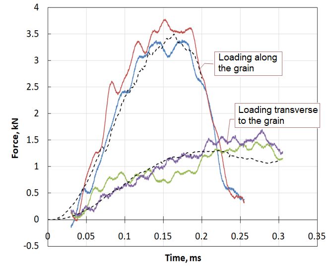
Materials 2020, 13, 5261                                                                                2 of 12

for various types of stress–strain states in a wide range of strain rates and temperatures, in order to
equip mathematical models of wood with parameters (identification) that can adequately describe the
behavior of the engineering structure containing wood components under shock wave loads.
      The first detailed review of using wood as an element of damping structures was given by
Johnson [2]. In the report, he noted that the dynamic properties of wood are not well understood.
In the past three decades, quite a lot of works have appeared that explored various aspects of the
high-speed deformation and destruction of wood, including the use of wood as a damping material in
containers for transportation of radioactive materials by air, road and rail transport [3]. A large amount
of research into the dynamic properties of wood was performed by Reid et al. [4–6]. In these works,
the dependences of destructive stress and energy absorption on the impact velocity were obtained.
      It was noted that dynamic destructive stresses are several times higher than static ones. The authors
also postulated that failure stresses of specimens fabricated along the grain are an order of magnitude
higher than that of the specimens cut transverse to the grain. The relationship between mechanical
parameters of selected wood species (Carya sp., Fagus sylvatica L., Acer platanoides L., Fraxinus excelsior L.,
Ulmus minor Mill.) and the grain orientation angle concern loading direction was investigated in [7].
It was observed that as the angle between fibers and loading direction increases whereas the mechanical
characteristics of all wood species decrease.
      In the works of Bragov et al., using the Kolsky method, dynamic diagrams of birch, aspen,
and sequoia were obtained at strain rates of ~103 s−1 with different direction of cutting specimens
relative to the direction of timber fibers [8,9]. The deformation diagrams of specimens under loading
along the grain are much higher than those under loading transverse to the grain. The limiting
deformative characteristics have the opposite direction.
      In recent years, interest in studying the effect of moisture, density and cutting angle on the
mechanical properties of wood has increased significantly. Adalian et al. [10] and Eisenacher et al. [11]
carried out a cycle of tests on wood in the range of strain rate from 10−3 to 103 s−1 . Wouts et al. [12],
Ha et al. [13,14] and Hao et al. [15] considered the damping ability of various biological materials
of plant origin from the point of view of improving artificial damping structures. Mach et al. [16]
calculated the hysteresis losses (dissipated energy) as the area bounded by the loading and unloading
curves, whereas stored energy (recoverable energy) is defined as the area under the unloading curve.
Thus, the total energy is calculated by summing the area of the hysteresis loss and the stored energy.
In the work of Novikov et al. [17], a large number of tests of sequoia, birch, aspen, and pine was
carried out at different cutting angles, temperatures ranged from −30 ◦ C to +65 ◦ C, and at the moisture
content of 5%, 20% and 30%. As a result, the dependence of strength on moisture and cutting angle
was determined.
      The mechanical properties of wood strongly depend on the place of growth, its age, the place of
cutting and the type of stress–strain state. Therefore, the results obtained by different authors may
differ significantly from each other. The purpose of this work is to conduct a detailed study of the
effect of strain rate and type of stress–strain state on the mechanical properties of wood as well as to
identify and verify the wood model.

2. Test Methods, Materials and Specimens
     For dynamic compressive tests of wood, the Kolsky method and split Hopkinson pressure bar
(SHPB) technology were used [18]. Figure 1 shows the installation diagram, as well as the main formulas
for determining the parametric dependencies of deformation, stress and strain rate of the sample under
compression. Two measuring bars were made of high-strength aluminum alloy and had a diameter of
20 mm and length of 1.5 m. During testing, a striker accelerated in the barrel of a gas gun impacts the
SHPB and excites an elastic compression wave in the loading measuring bar, which, upon reaching the
specimen, deforms it. The second (support) measuring bar acts as a dynamometer-waveguide and
allows you to register the transmitted strain pulse εT (t) and then to determine the process of stress
developing in the specimen. The pulse εR (t) reflected from the specimen in the loading bar makes it
Materials 2020, 13,
Materials 2020, 13, 5261
5261 33 of
of 12
12
specimen, and its integration allows to determine the process of the specimen deformation
possible to determine the process of strain rate change in the specimen, and its integration allows to
development. Small-length foil strain gages were used for registration elastic strain pulses in the bars.
determine the process of the specimen deformation development. Small-length foil strain gages were
Based on these pulses, the parametric processes of stress, strain and strain rate over time are
used for registration elastic strain pulses in the bars. Based on these pulses, the parametric processes of
calculated using the formulae shown in the lower part of Figure 1. Then, excluding time as a
stress, strain and strain rate over time are calculated using the formulae shown in the lower part of
parameter, a dynamic stress–strain curve is constructed with the known law of variation of the strain
Figure 1. Then, excluding time as a parameter, a dynamic stress–strain curve is constructed with the
rate [19].
known law of variation of the strain rate [19].
Figure 1. Installation scheme and basic dependencies.
Figure 1. Installation scheme and basic dependencies.
Dynamic tests were carried out with specimens of lime-tree (Tilia europoea) and pine (Pinaceae)
with aDynamic
diametertests
of 20were carried
mm and out with
a length of 10specimens
mm, cut from of lime-tree
solid wood(Tilia europoea)
at an 0◦ and
angle ofand pine ◦ relative
90(Pinaceae)
with
to theaaxis
diameter of 20trunk.
of the tree mm andThe aflat
length
ends of the
10 mm, cut from
samples solid wood
were carefully at an angle before
hand-grinded of 0° and 90°
testing.
relative
The to theparameters
physical axis of the of
tree trunk.
tested The flatare
materials ends of theinsamples
shown were
the Table 1. carefully hand-grinded before
testing. The physical parameters of tested materials are shown in the Table 1.
Table 1. The physical parameters of tested materials.
Table 1. The physical parameters of tested materials.
Wood Species Lime-Tree Pine
Wood Species
Parameter Along the GrainLime-Tree
Transverse to the Grain Along the Grain Pine
Transverse to the Grain
Parameter 3 Along the Grain Transverse to the Grain Along the Grain Transverse to the Grain
Density, g/cm 0.505 ± 0.02 0.512 ± 0.015 0.435 ± 0.01 0.484 ± 0.015
Density, g/cm3 0.505 ± 0.02 0.512 ± 0.015 0.435 ± 0.01 0.484 ± 0.015
Moisture content,%%
Moisture content, 7.5 ± 0.2
7.5 ± 0.2 7.9±±0.3
7.9 0.3 6.8 ±± 0.3
6.8 0.3 7.1±± 0.2
7.1 0.2
The total
The totalamount
amountofoftested
tested samples
samples of of
eacheach wood
wood species
species amounted
amounted 50 pieces:
50 pieces: 40 pieces
40 pieces were were
used
used
for for mechanical
mechanical testing
testing and 10and 10 pieces
pieces were were
used used for subsequent
for subsequent woodwood
model model verification.
verification. In each
In each test
test mode during mechanical testing (strain rate and loading direction), 4–5 experiments
mode during mechanical testing (strain rate and loading direction), 4–5 experiments were carried out, were carried
out,results
the the results of which
of which were
were then then averaged.
averaged. All the experiments
All the experiments were
were carried outcarried out in conditions
in laboratory laboratory
conditions
at at room temperature
room temperature and 50% airand 50% air humidity.
humidity.
3.
3. Experimental Results
Using abovemethods,
Using the above methods,the thedynamic
dynamic tests
tests of pine
of pine andand lime-tree
lime-tree werewere carried
carried out. Asout.a result,
As a
result,
their dynamic stress–strain curves, the ultimate strength and deformative characteristics of the
their dynamic stress–strain curves, the ultimate strength and deformative characteristics of the
specimens
specimens cut cutalong
alongand
andtransverse
transverse toto
thethe
grain were
grain wereobtained. Dynamic
obtained. Dynamic strain diagrams
strain diagramsfor pine and
for pine
lime-tree underunder
and lime-tree uniaxial stress stress
uniaxial state are presented
state in Figures
are presented 2 and 3. 2The
in Figures and figures
3. Theshow the averaged
figures show the
stress–strain curves and appropriate strain rate-strain curves. The spread of the obtained
averaged stress–strain curves and appropriate strain rate-strain curves. The spread of the obtained properties
was no more
properties than
was no6%.
moreIn than
all figures
6%. Insolid lines show
all figures solidthe dependences
lines of the true stress
show the dependences of the
of the truespecimen
stress ofMaterials 2020, 13, 5261 4 of 12
Materials 2020, 13, 5261 4 of 12
Materials 2020, 13, 5261 4 of 12
the specimen on its deformation σ~ε, and the dotted lines (in the lower part of the diagrams)
on its deformation σ~ε, and the dotted lines (in the lower part of the diagrams) correspond to the
the specimen
correspond to on
the its deformation
history σ~ε,rate
of the strain andchange
the dotted lines
έ~ε (the (in the lower
appropriate axis ispart of right).
on the the diagrams)
history of the strain rate change έ~ε (the appropriate axis is on the right).
correspond to the history of the strain rate change έ~ε (the appropriate axis is on the right).
Figure 2. Deformation diagrams of pine under loading along and across the grain.
Figure
Figure 2. Deformation diagrams
2. Deformation diagrams of
of pine
pine under
under loading
loading along
along and
and across
across the
the grain.
grain.
Figure 3. Deformation diagrams of lime-tree under loading along and across the grain.
Figure 3. Deformation diagrams of lime-tree under loading along and across the grain.
Figure
Two test 3. Deformation
modes diagrams
on strain rate of lime-tree
were chosen: with under loading along
non-destructive andand across the results.
destructive grain. From the
Twostress–strain
obtained test modes on strain rate
diagrams, were chosen:
it follows that forwith
bothnon-destructive
wood species the andspecimens
destructive cutresults.
and loadedFrom
the Two test
obtained modes on
stress–strain strain rate
diagrams, were it chosen:
follows with
that non-destructive
for both wood and
species
along the grain have the largest modulus of the load branch in the diagram, as well as ultimate stress destructive
the specimensresults.cutFrom
and
the obtained
loaded
and along
energy stress–strain diagrams, it follows that for both wood species
the grain have the largest modulus of the load branch in the diagram, as well as ultimate
absorption. the specimens cut and
loaded
stress along
and the
energy
Wood endurance grain have
absorption.
can be theindicated
largest modulusin Figure of the load branch
4, where diagramsin the
ofdiagram,
fivefold as well asofultimate
loading a pine
stress and energy absorption.
specimen with its minor damages (curves 1–5) and a single independent loading of anotherofsimilar
Wood endurance can be indicated in Figure 4, where diagrams of fivefold loading a pine
Wood
specimenwith
specimen endurance
withitsitscomplete can be
minor damages indicated
(curves
failure (curve in Figure
1–5)
6) are 4, where
and a single
presented. diagrams
independent
The diagrams of fivefold
loadingon
are located loading
oftheanother of a pine
similar
deformation
specimen
specimen
axis with
withitsits
conditionally minor
in order damages
complete (curves
failure
to make (curve
it easier 1–5)
6)andareathe
to assess single
effectindependent
presented. loadingare
The diagrams
of multiple loading of the
on another
located similar
on the
steepness of
specimen
deformation
the with
load sections its complete
axisofconditionally failure
the stress–strain in order (curve
curves.toThe 6)
make are presented.
it easier
average The
to assess
strain diagrams
rate at the effectloads
repeated are located
of multiple loadingsthe
was ~600–800 on on,
−1
deformation
the steepnessaxisof the conditionally
load sections inoforder to make it easier
the stress–strain curves. to The
assess the effect
average ofrate
strain multiple loading
at repeated on
loads
the
wassteepness
~600–800of s−1the load
, and sections
in the case ofofspecimen
the stress–strain
failure, curves.
the strain The average
rate strain
was about rates−1
2200 at. One
repeated loads
can clearly
was ~600–800 s−1, and in the case of specimen failure, the strain rate was about 2200 s−1. One can clearlyMaterials 2020, 13, 5261 5 of 12
Materials 2020, 13, 5261 5 of 12
Materials 2020, 13, 5261 5 of 12
see a decrease in the steepness of the load section of stress–strain curve during repeated loads by a
and in the case of specimen failure, the strain rate was about 2200 s−1 . One can clearly see a decrease
factor
see of 2–3, which
a decrease in the is associated
steepness withload
of the partial destruction
section of the specimen
of stress–strain during
curve during each loading
repeated and
loads by a
in the steepness of the load section of stress–strain curve during repeated loads by a factor of 2–3,
violation
factor of the
of 2–3, flatness
which of its ends.
is associated with partial destruction of the specimen during each loading and
which is associated with partial destruction of the specimen during each loading and violation of the
violation of the flatness of its ends.
flatness of its ends.
Figure 4. An example of multiply repeated loading of the specimen with its minor damage.
Figure 4. An example of multiply repeated loading of the specimen with its minor damage.
Figure 4. An example of multiply repeated loading of the specimen with its minor damage.
As an
As animportant
importantcharacteristic
characteristicof of
thethe timber
timber damping
damping capacity,
capacity, the energy
the energy absorption
absorption of the of the
tested
tested
wood wood
Asspeciesspecies
an important was estimated
characteristic
was estimated under
of the loading
under loading timber along
damping
along and andcapacity,
transverse
transverse to thethe toenergy
grain the
bygrain by calculating
absorption
calculating ofarea
the the
the area
tested under
wood the curve
species was σ~ε (Figure
estimated
under the curve σ~ε (Figure 5). 5).
under loading along and transverse to the grain by calculating
the area under the curve σ~ε (Figure 5).
a) b)
a) b)
Figure
Figure 5. Energy absorption
5. Energy absorption of
of the
the tested
tested wood
wood species:
species: (a)
(a) for
for pine,
pine, (b)
(b) for
for lime-tree.
lime-tree.
Figure 5. Energy absorption of the tested wood species: (a) for pine, (b) for lime-tree.
For both wood species, there is a significant excess of energy absorption by the specimens cut and
For both wood species, there is a significant excess of energy absorption by the specimens cut
tested along the grain, compared to the specimens cut and tested transverse to the grain.
and tested
For both along
woodthespecies,
grain, compared
there is ato the specimens
significant excesscutof and
energy tested transverse
absorption bytothethespecimens
grain. cut
It is interesting to compare the results on the damping ability of wood-based materials obtained
It is interesting
and tested along the to compare
grain, comparedthe results
to theon the damping
specimens ability
cut and testedof wood-based
transverse tomaterials
the grain.obtained
by other researchers. In the work [12] the damping capacity of two types of deciduous and coniferous
by other researchers.toIncompare
It is interesting the workthe [12] the damping
results capacity ability
on the damping of two of types of deciduous
wood-based and coniferous
materials obtained
wood: beech and spruce under loading in the longitudinal, tangential and radial directions were
wood:
by otherbeech and spruce
researchers. In theunder
work [12]loading in the longitudinal,
the damping capacity of two tangential
types ofand radial directions
deciduous were
and coniferous
compared. The highest specific energy absorbed was noted for specimens under longitudinal loading,
compared.
wood: beechTheandhighest
spruce specific energyinabsorbed
under loading was noted
the longitudinal, for specimens
tangential under
and radial longitudinal
directions were
and the smallest—under tangential loading. This is traditional tendency for wood materials.
loading, andThe
compared. the highest
smallest—under
specific tangential
energy absorbedloading.was
This noted
is traditional tendencyunder
for specimens for wood materials.
longitudinal
While
While in [14], the damping ability of the mesocarp layer in durian shell (tropical fruit)
fruit) was
loading, andinthe[14], the damping tangential
smallest—under ability of loading.
the mesocarp
This islayer in durian
traditional shell for
tendency (tropical
wood materials.was
investigated
investigated and, as aa result of
of the research, it was found the
the inverse
inverse effect:
effect: specific
specific energy
energy absorption
While inand, [14],asthe result
damping theability
research,of itthe
was found
mesocarp layer in durian shell (tropical absorption
fruit) was
of the mesocarp
investigated and,layer underoflateral
as a result loadingitis
the research, higher
was found than
the that
inverseunder axial
effect: one. This
specific energymayabsorption
be due to
of the mesocarp layer under lateral loading is higher than that under axial one. This may be due toMaterials 2020, 13, 5261 6 of 12
of the mesocarp layer under lateral loading is higher than that under axial one. This may be due to
the fact that the durian shell does not have the same clearly pronounced fiber structure as in wood,
therefore the authors’ accentuation on the lower strength and damping ability of the material in the
axial direction of load application compared to lateral loading refers to the radial and tangential
strength of shell of this fruit.
4. Identification and Verification of the Wood Model
To describe the behavior of wood under dynamic loads in the library of the LS-DYNA calculation
complex, there is model No. 143 MAT_WOOD. This is a model of a transversely isotropic material for
solid elements. It is possible to set material properties or use a predefined set of constants, but only for
two species of pine growing in the USA: southern yellow pine and Douglas fir.
The primary features of the model are:
• Transverse isotropy for the elastic constitutive equations (different properties are modeled parallel
and perpendicular to the grain).
• Yielding with associated plastic flow formulated with separate yield (failure) surfaces for the
parallel- and perpendicular-to-the-grain modes.
• Hardening in compression formulated with translating yield surfaces.
• Post-peak softening formulated with separate damage models for the parallel and
perpendicular-to-the-grain modes.
• Strength enhancement at high strain rates.
Model 143 for pine contains a predefined set of 29 parameters depending on moisture content and
temperature. According to the results of the pine tests, some parameters of this model were adjusted
for a particular batch of samples under study. These parameters are shown in Table 2.
Table 2. Main mechanical properties of pine for model identification.
Designation Value
Density 450 kg/m3
Modulus of elasticity in the direction of the grain 10,500 MPa
Flow stress during compression in the direction of the grain 80 MPa
The modulus of elasticity in the direction perpendicular to the grain 246 MPa
Flow stress during compression in the direction perpendicular to the grain 10 MPa
It should be noted that the elastic moduli of pine under loading along and across the grain
were obtained as a result of quasi-static tests, since the Kolsky method, in principle, does not allow
constructing a stress–strain curve in which the slope dσ/dε of the elastic loading section would be
equal to the static modulus of elasticity. Usually the steepness of this section is several times less than
the static Young’s modulus. The reasons for this are as follows:
- The difference in the cross-sectional areas of the measuring bars and the sample (some part of
the incident wave is reflected from the free surface around the sample), causing an apparent
deformation of the sample,
- The presence of gaps between the ends of the measuring bars and the sample (due to the
non-parallelism of its ends and their roughness or insufficient “pressing” of the sample during
the preparation of the test),
- Dispersion during the propagation of waves in the bars (decrease in the steepness of the transmitted
pulse during the propagation time to the recording strain gauge).
In order to confirm the adequacy of the model parameters determined from experiments,
it is necessary to verify it, but in experiments other than those in which these parameters wereMaterials 2020, 13, 5261 7 of 12
obtained. For
Materials 2020, 13,this
5261purpose, we used a model experiment in full-scale and numerical implementation. 7 of 12
The simulation of the indentation process was performed using the finite element method. The explicit
Materials
performed
time 2020,
integration 13, 5261
using the
schemeDynamics-2
was used for solving the equations of motion in time. Modeling 7was
® software package [20]. The numerical experiment was simulated of 12
in an axisymmetric formulation,
performed using the Dynamics-2 software ®and its design corresponded to a similar natural test.
package [20]. The numerical experiment was simulated in
performed
To verify usingthe the Dynamics-2
model of and
® software package [20]. The numerical experiment was simulated
material behavior, we usedtoan experimental scheme for dynamic
an axisymmetric formulation, its design corresponded a similar natural test.
in an axisymmetric
indentation by using formulation,
the system ofanda its design
split corresponded
Hopkinson bar. The to a similarprocedure
indicated natural test.is schematically
To verify the model of material behavior, we used an experimental scheme for dynamic indentation
shown To verify the model of material behavior, we used an experimental scheme forhead
dynamic
by usinginthe Figure
system 6. ofThe sample
a split 5 and abar.
Hopkinson removable indenter
The indicated 4 with ais hemispherical
procedure schematically shown are
in
indentation
sandwiched by using
between the
the system
measuring of a
barssplit
2 Hopkinson
and 6. Upon bar.
impact The indicated
loading by procedure
the striker 1,is
a schematically
compression
Figure 6. The sample 5 and a removable indenter 4 with a hemispherical head are sandwiched between
shown is
impulse ingenerated
Figure 6. inThe sample 5 duration
and a removable indenteron 4 the
with a hemispherical head are
the measuring bars 2 andthe bar 2 the
6. Upon impact loadingof which depends
by the striker length
1, a compression of the striker
impulse and the
is generated
sandwiched
amplitude between theofmeasuring bars 2 and 6. Upon impact loading by the the striker 1, a compression
in the bar 2on thethe speed
duration the striker.
of which depends In the case
on the of hemispherical
length of the strikerindenter, contact
and the amplitude onarea at the
the speed
impulse
initial is
moment generated
of in the
indentation baris 2 the
very duration
small, of which
therefore, thedepends
amplitudeon the
of length
the of the
reflected striker
pulse and
is verythe
of the striker. In the case of hemispherical indenter, the contact area at the initial moment of indentation
amplitude and
significant, on theso speed of theisstriker.
the sample loaded In the case of hemispherical indenter, oftheadditional
contact area at the
is very small, therefore, the amplitude of several times.
the reflected For reliable
pulse recording
is very significant, and so the sample loading is
initial
cycles, itmoment
is necessaryof indentation
to increase is very small, therefore,
the lengthofofadditional the
the supporting amplitude
bar of the
in comparison reflected pulse
withtothe lengthvery
is of
loaded several times. For reliable recording loading cycles, it is necessary increase the
significant,
the loading andasso the sample is loaded several times.cycles
For reliable recording of additional loading
length of thebar much
supporting as
barrequired to register
in comparison withloading
the length [21].loading
of the bar as much as required to
cycles, it is necessary to increase the length of the supporting bar in comparison with the length of
register loading cycles [21].
the loading bar as much as required to register loading cycles [21].
Figure 6. High speed indentation experiment scheme.
Figure 6. High speed indentation experiment scheme.
Using strain gauges 3,Figure elastic6. strain
High speed
pulses indentation
are recordedexperiment
in thescheme.
measuring bars (Figure 7). The
Usingpulses
following strainaregauges
indicated3, elastic strain 1—incident
by numbers: pulses are recorded in thepulse
(loading) strain measuring bars (Figure
εI(t), 2—reflected pulse7).
Using strain gauges R3, elasticby strain pulses1—incident
are recorded in theI measuring bars (Figure
I (t), 7). The
in the first loading cycle ε1 (t ) , 3—incident (loading) strain pulse ε 2 (t ) in the second
The following pulses are indicated numbers: (loading) strain pulse ε 2—reflected
loading cycle,
following
pulse in thepulses are indicated
first loading cycle εby R (numbers:
t), 3—incident1—incident
(loading) (loading)
strain strain
pulse pulse εI(t),
εI2 (t) in the2—reflected
second loading pulse
R T
4—reflected
cycle, strain
in the4—reflected
pulse
first loading strain
in the
cycle pulse
R
1
second loading
ε1 (t ) ,in3—incident cycle
the second(loading) ε 2
loading strain(t ) , 5—transmitted
cycle εpulseR I pulse (first
ε 2 (t ) in the second
(t), 5—transmitted cycle)
pulseloading ε 1 (t )
(first cycle)
cycle,
T
2
T
ε, 14—reflected
6—transmitted
(t), 6—transmittedpulsepulse
(second
strain pulse
ε 2loading
cycle)cycle)
in(second
the second
(tε)2.(t). cycle ε R (t ) , 5—transmitted pulse (first cycle) ε T (t )
T
2 1
T
, 6—transmitted pulse (second cycle) ε (t ) . 2
Figure 7. Typical waveform obtained in the experiment for high-speed indentation, taking into account
Figure 7. Typical waveform obtained in the experiment for high-speed indentation, taking into
additional cycles: upper beam—data from bar 2; lower beam—data from bar 6.
account additional cycles: upper beam—data from bar 2; lower beam—data from bar 6.
Figure 7. Typical waveform obtained in the experiment for high-speed indentation, taking into
The loading of the SHPB system in the numerical experiment (Figure 8) is performed in the same
account
The additional
loading cycles: system
of the SHPB upper beam—data from bar
in the numerical 2; lower beam—data
experiment (Figure 8)from bar 6.
is performed in the same
way as in the natural experiment—with the help of a striker having an initial velocity V 0 . In the
way as in the natural experiment—with the help of a striker having an initial velocity V0. In the
The loading
calculation ofthe
process, theincident
SHPB system in the numerical
and reflected experiment
strain pulses (Figurein8)element
are calculated is performed
2 and in
thethe same
past—
way as in the natural experiment—with the help of a striker having an initial
in element 6. The time dependences obtained during the simulation are compared with the velocity V 0. In the
calculation process,
corresponding valuesthe incidentduring
recorded and reflected strain pulses are calculated in element 2 and the past—
the experiment.
in element 6. The time dependences obtained during the simulation are compared with the
corresponding values recorded during the experiment.Materials 2020, 13, 5261 8 of 12
Materials 2020, 13, 5261 8 of 12
calculation process, the incident and reflected strain pulses are calculated in element 2 and the past—in
element 6. The time dependences obtained during the simulation are compared with the corresponding
Figure 8. High speed indentation experiment simulation scheme.
Materialsrecorded
values 2020, 13, 5261
during the experiment. 8 of 12
The indenter is made of high-strength tungsten–cobalt alloy and is modeled by a rigid non-
deformable material.
To assess the processes occurring in the sample, data obtained from measuring bars is used. In
accordance with the Kolsky formulas, one can calculate the law of change of the indenter penetration
rate into the sample V(t) and the penetration resistance force F(t):
Figure 8. High speed
V(t) =indentation
C1·(εI(t) + εexperiment
R(t)) − C2·εsimulation
T(t) scheme.
Figure 8. High speed indentation experiment simulation scheme.
(1)
The indenter is made of high-strength F(t) =tungsten–cobalt
E2∙S2 εT(t). alloy and is modeled by a rigid
The indenter
non-deformable is made of high-strength tungsten–cobalt alloy and is modeled by a rigid non-
material.
here εI(t), εR(t)
deformable and εT(t) denote the incident, reflected, and transmitted strain pulses in the measuring
material.
To assess the processes occurring in the sample, data obtained from measuring bars is used.
bars, respectively,
To assesswith the Ethe
is the elastic
processes modulus,the and C is thedata
bar obtained
velocity of sound. The subscripts 1 and In 2
In accordance Kolskyoccurring
formulas, in one can sample,
calculate the law of change from measuring
of the indenter barspenetration
is used.
refer to
accordance the first (loading) and second (supporting) measuring bars.
rate into the with sample theV(t)
Kolskyandformulas,
the penetrationone can calculateforce
resistance the lawF(t):of change of the indenter penetration
rate When
into the modeling
sample V(t) the and
process of dynamic resistance
the penetration indentation intoF(t):
force wood samples, the following scheme
was used: a sample and an indenter V(t) = were
C1C·(εconsidered
I (t) + εR (t))(Figure
− C 2·ε 9). The spatial discretization of the
·εTT(t)
(t)
1·(εI(t) + εR(t)) − C2
indenter and the sample was doneV(t) by=using a solid
F(t) = E2 ·S2 ε (t). T three-dimensional finite element with one (1)
(1)
integration point. Due to the presence of symmetry, F(t) = E2∙S a 2quarter
ε (t). of the geometric model was considered.
T
On
here the I planesR of symmetry,
T the corresponding boundary conditions were pulses specified:the at the nodes
hereεεI(t),
(t), εεR(t) and εεT(t)
(t) and (t) denote
denote thethe incident,
incident, reflected,
reflected, and and transmitted
transmitted strain strain pulses in in the measuring
measuring
lying on the plane with the normal in the direction of the oY axis, zero velocities in the oY direction2
bars, respectively,EEisisthe
bars,respectively, theelastic
elasticmodulus,
modulus,and andCCisisthe thebar
barvelocity
velocityof ofsound.
sound.The Thesubscripts
subscripts11and and 2
and
refer zerothe velocities of rotation about the oX and oZ axes were set; at the nodes lying on the plane with
referto to thefirst
first(loading)
(loading)and andsecond
second(supporting)
(supporting)measuringmeasuringbars. bars.
the normal
When in the direction of the oZ axis, zero velocitiesintoin the oZ direction
the and zero velocities of
Whenmodeling
modelingthe theprocess
process ofof
dynamic
dynamic indentation
indentation wood
into wood samples,
samples, following
the followingscheme was
scheme
rotation
used: about
a sample the oX
and anandand oY
indenter axes were set.
were considered (Figure (Figure
9). The spatial
was used: a sample an indenter were considered 9). Thediscretization of the indenter
spatial discretization of the
and Zero
the velocities
sample was in theby
done direction
using a of thethree-dimensional
solid oX axis were set at the element
finite nodes belonging
with one to the surface
integration of
point.
indenter and the sample was done by using a solid three-dimensional finite element with one
the
Due sample, which
to the presence in full-scale
of symmetry, experiments
a quarter rested against
of the geometric the transmitted measuring bar.
integration point. Due to the presence of symmetry, a quartermodelof thewas considered.
geometric modelOn wasthe planes of
considered.
The indenter
symmetry, was modeledboundary by an absolutely rigid undeformable body. For thelying
indenter, the law
On the planes of symmetry, the corresponding boundary conditions were specified: at the plane
the corresponding conditions were specified: at the nodes on the nodes
of thethe
with change
normal ininthethespeed of itsofmovement
direction the oY axis, inzerothe velocities
axial direction
in the was
oY set. The and
direction timezerodependence
velocities of
of
lying on the plane with the normal in the direction of the oY axis, zero velocities in the oY direction
indenter’s
rotation axial
about velocity
the oX and foroZa particular
axes were experiment
set; at the was
nodes calculated
lying on using
the the
plane Equation
with the (1)
normal based
in on
the
and zero velocities of rotation about the oX and oZ axes were set; at the nodes lying on the plane with
the signals
direction ofrecorded
the in the
oZ axis, zero measuring
velocities bars.
the normal in the direction of the oZ in thezero
axis, oZ direction
velocitiesand zerooZ
in the velocities
direction of and
rotation
zeroabout the oX
velocities of
and The
oY “surface–surface”
axes were set. contact interaction was set between the indenter and the sample.
rotation about the oX and oY axes were set.
Zero velocities in the direction of the oX axis were set at the nodes belonging to the surface of
the sample, which in full-scale experiments rested against the transmitted measuring bar.
The indenter was modeled by an absolutely rigid undeformable body. For the indenter, the law
of the change in the speed of its movement in the axial direction was set. The time dependence of
indenter’s axial velocity for a particular experiment was calculated using the Equation (1) based on
the signals recorded in the measuring bars.
The “surface–surface” contact interaction was set between the indenter and the sample.
a) b)
Figure 9.9.Geometric statement
Geometric of the
statement of problem of numerical
the problem simulation:
of numerical (a) 3D configuration,
simulation: (b) plane
(a) 3D configuration,
configuration.
(b) plane configuration.
Zero velocities in the direction of the oX axis were set at the nodes belonging to the surface of the
sample, which in full-scale experiments rested against the transmitted measuring bar.
The indenter was modeled by an absolutely rigid undeformable body. For the indenter, the law
of a)
the change in the speed of its movement in the axial b)direction was set. The time dependence of
Figure 9. Geometric statement of the problem of numerical simulation: (a) 3D configuration, (b) plane
configuration.Materials 2020, 13, 5261 9 of 12
indenter’s axial velocity for a particular experiment was calculated using the Equation (1) based on the
signals recorded in the measuring bars.
Materials 2020, 13, 5261 9 of 12
The “surface–surface” contact interaction was set between the indenter and the sample.
InInnatural
naturalexperiments
experiments on on the
the indentation thesamples
indentation the samplesofofpinepinewere
wereused
used ininthethe form
form of of tablets
tablets
with
with a length of 10 mm and a diameter of 20 mm. Some of the samples were cut in the directionof
a length of 10 mm and a diameter of 20 mm. Some of the samples were cut in the direction ofthe
wood grain,grain,
the wood whilewhile
another partpart
another of the samples
of the waswas
samples cutcut
in in
thethe
perpendicular
perpendiculartotothethegrain
graindirection.
direction.
AsAs mentioned
mentionedabove,above,ininthe
the process
process of dynamic
dynamicindentation,
indentation,the thesample
sample is is subjected
subjected to to multiple
multiple
loading
loading ininthe
theexperiment
experiment(see(seeFigure
Figure 7), thus
thusundergoing
undergoingaacertain
certaindeformation
deformation in in each
each loading
loading cycle.
cycle.
High-speed
High-speed filmfilm recording
recording of the
of the indentation
indentation process
process makes
makes it possible
it possible to estimate
to estimate a number
a number of
of loading
loading
cycle and cycle and indentation
indentation depth atdepth
which at which the destruction
the destruction of theofmaterial
the material occurs.
occurs. Figure
Figure 1010shows
showsthe
the frames
frames of such of such registration,
registration, made made
usingusing a high-speed
a high-speed camera
camera HSFCHSFC Pro.
Pro.
Figure 10. High-speed
Figure10. registrationofofdynamic
High-speed registration dynamicindentation.
indentation.
TheThe left part
left of of
part thethe
figure corresponds
figure corresponds to the experiment
to the experiment with thethe
with sample cutcut
sample in the direction
in the along
direction
thealong
grain, whereas the right part corresponds to the experiment with the
the grain, whereas the right part corresponds to the experiment with the sample cut in the sample cut in the direction
transverse
direction to the grain.
transverse to The numbers
the grain. Theon the left on
numbers of the
the high-speed registration
left of the high-speed images indicate
registration imagesthe
number
indicate ofthe
loading
number cycles (running
of loading number
cycles of impulse
(running numberinof the loadinginmeasuring
impulse the loadingbar) which one
measuring bar)can
seewhich
in Figure 7. It can be seen in Figure 10 that the samples cutting off parallel to
one can see in Figure 7. It can be seen in Figure 10 that the samples cutting off parallel to thethe grain remain intact
throughout
grain remain theintact
experiment,
throughout whichtheisexperiment,
confirmed by the final
which state of such
is confirmed by thesamples. Samples
final state of such obtained
samples. by
cutting
Samples in the direction
obtained perpendicular
by cutting to the grain
in the direction retain their
perpendicular integrity
to the duringtheir
grain retain the integrity
first loading cycle,
during
however,
the first cracks
loadingand cycle,gaps between
however, the layers
cracks and gapsof wood
between appear in theofsecond
the layers cycle, which
wood appear in the grow
secondand
cycle, which
progress grow and loading
in subsequent progresscycles,
in subsequent
leadingloading cycles, leading
to the separation of theto sample
the separation of the sample
into parts.
intoIt parts.
can be noted that for the same load amplitude, the samples obtained by cutting in the direction
It canremain
of the fiber be noted that for
intact, thethe
while same load amplitude,
samples the samples
cut perpendicular obtained
to the by cutting
fiber exhibit in the
failure direction
already in the
of the fiber
first loading cycle.remain intact, while the samples cut perpendicular to the fiber exhibit failure already in
the first loading cycle.
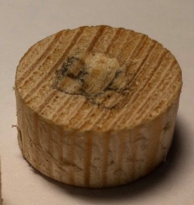
A comparison of the shape of the imprint on the pine sample after the experiment on the
dynamic indentation of a hemispherical indenter is shown in Figure 11.Materials 2020, 13, 5261 10 of 12
A comparison of the shape of the imprint on the pine sample after the experiment on the dynamic
indentation
Materials 2020,
Materials of 5261
2020, 13,
13, a hemispherical indenter is shown in Figure 11.
5261 10 of
10 of 12
12
a) b)
Figure 11.
Figure11.
Figure The shape
Theshape
11.The ofofthe
shapeof the imprints
theimprints obtained
imprintsobtained by
obtainedby numerical
bynumerical modeling
numericalmodeling (a)
modeling(a) and
(a)and in
andin the
inthe natural
thenatural test
naturaltest (b).
test(b).
(b).
Figure 12 shows
Figure shows a comparison
comparison of the time dependences
dependences of the indentation resistance
resistance of pine
sample recorded in the experiments (solid colored lines) with the data obtained by numerical
sample recorded in the experiments (solid colored lines) with the data obtained by numerical modeling
(black dashed lines) during dynamic indentation of hemispherical indenter into specimen both
modeling (black dashed lines) during dynamic indentation of hemispherical indenter into specimen along
and across
both along the
andgrain.
across the grain.
Figure 12.
Figure Comparison of
12. Comparison of experimental
experimental and
and calculated
calculated pulses
pulses in
in the
the supporting
supporting bar.
bar.
Figure 12. Comparison of experimental and calculated pulses in the supporting bar.
It can be seen that the model used allows us to accurately reproduce the features of the deformation
It can be seen that the model used allows us to accurately reproduce the features of the
of real material, namely, the difference in its deformation behavior in different directions with respect
deformation of real material, namely, the difference in its deformation behavior in different directions
to grain orientation.
with respect to grain orientation.
The results obtained are in qualitative agreement with the data from previous studies of high
The results obtained are in qualitative agreement with the data from previous studies of high
strain rate behavior of wood [8,17]. Correction of some parameters of the MAT_WOOD model made it
strain rate behavior of wood [8,17]. Correction of some parameters of the MAT_WOOD model made
it possibletotodescribe
possible describethe
thedeformation
deformationbehavior
behaviorof of the
the studied
studied wood species with
wood species with sufficient
sufficientaccuracy.
accuracy.
A further increase in the quality of the mathematical model is possible by taking into account the effect
A further increase in the quality of the mathematical model is possible by taking into account the
of the of
effect strain rate inrate
the strain a wide
in arange
wideof its change,
range as well as
of its change, as well
taking
asinto account
taking the fracture
into account of the material.
the fracture of the
material. In addition, it is necessary to conduct more complex model experiments to verify the
fracture criteria, for example, high-speed penetration and perforation of wood plates.Materials 2020, 13, 5261 11 of 12
In addition, it is necessary to conduct more complex model experiments to verify the fracture criteria,
for example, high-speed penetration and perforation of wood plates.
5. Conclusions
Dynamic tests of lime-tree and pine were conducted. There is a strong anisotropy of the properties
of the tested materials: the specimens exhibit the greatest strength under load applied along the
grain, while the lowest strength is observed under loading transverse to the grain. The load branch
module is non-linear and, as a rule, smaller than the unloading branch module (while maintaining the
specimen integrity). At the specimen cutting angle of 90◦ with respect to the direction of the fibers,
the stress–strain diagram after reaching a certain threshold stress value (about 8 MPa for lime-tree
and about 10 MPa for pine) is close to the ideal plastic diagram. At 0◦ cutting angle, the initial section
of the diagrams is close to linear. That is, an elastic deformation occurs. However, after reaching an
ultimate stress value (yield strength), the diagram becomes nonlinear with stress relaxation. Especially
such behavior is observed in the experiments in which the failure of specimens occurs.
Using a modification of the SHPB method, experiments were performed on the dynamic
indentation of indenters with a hemispherical head into the samples parallel and perpendicular
to the direction of the fibers. Dependences of resistance to penetration on time are constructed. In the
direction of the fiber (along the grain), the resistance force was more than three-times greater than
in the transverse direction. The results of the natural experiment were compared with the results of
numerical modeling, in which the wood behavior was described by the MAT_WOOD model from
the LS-DYNA software, in which some of the parameters were obtained experimentally. A good
coincidence was observed.
Author Contributions: Conceptualization, A.B. and L.I.; data curation, T.I.; formal analysis, A.K.; funding
acquisition, L.I.; investigation, A.L.; methodology, A.K. and A.L.; project administration, A.B.; resources, L.I.;
software, A.K. and T.I.; supervision, F.d.; validation, F.d. and A.K.; visualization, A.K.; writing—original draft, A.L.;
writing—review and editing, A.B. All authors have read and agreed to the published version of the manuscript.
Funding: Experimental investigations of wood were performed with the financial support of the Ministry of
Science and Higher Education of the Russian Federation (task 0729-2020-0054). Numerical simulation of wood
behavior was supported by the grant of the Government of the Russian Federation (contract No.14.Y26.31.0031).
Conflicts of Interest: The authors declare no conflict of interest. The funders had no role in the design of the
study; in the collection, analyses, or interpretation of data; in the writing of the manuscript, or in the decision to
publish the results.
References
1. Murray, Y.D. Manual for LS-DYNA Wood Material Model 143; Publication No. FHWA-HRT-04-097; Federal
Highway Administration: Washington, DC, USA, 2007.
2. Johnson, W. Historical and present-day references concerning impact on wood. Int. J. Impact Eng. 1986,
4, 161–174. [CrossRef]
3. Neumann, M. Investigation of the Behavior of Shock-Absorbing Structural Parts of Transport Casks Holding
Radioactive Substances in Terms of Design Testing and Risk Analysis. Ph.D. Thesis, Bergische Universität
Wuppertal, Wuppertal, Germany, 2009.
4. Reid, S.R.; Reddy, T.Y.; Peng, C. Dynamic compression of cellular structures and materials. In Structural
Crashworthiness and Failure; Jones, N., Wierzbicki, T., Eds.; Taylor & Francis Publication: London, UK;
New York, NY, USA, 1993; pp. 257–294.
5. Reid, S.R.; Peng, C. Dynamic Uniaxial Crushing of Wood. Int. J. Impact Eng. 1997, 19, 531–570. [CrossRef]
6. Harrigan, J.J.; Reid, S.R.; Tan, P.J.; Reddy, T.Y. High rate crushing of wood along the grain. Int. J. Mech. Sci.
2005, 47, 521–544. [CrossRef]
7. Mania, P.; Siuda, F.; Roszyk, E. Effect of Slope Grain on Mechanical Properties of Different Wood Species.
Materials 2020, 13, 1503. [CrossRef] [PubMed]
8. Bragov, A.M.; Lomunov, A.K. Dynamic properties of some wood species. J. Phys. IV 1997, 7, 487–492.
[CrossRef]Materials 2020, 13, 5261 12 of 12
9. Bragov, A.M.; Lomunov, A.K.; Sergeichev, I.V.; Gray, I.I.I.G.T. Dynamic behaviour of birch and sequoia at
high strain rates. “Shock Compression of Condensed Matter”. In Proceedings of the Conference of the
American Physical Society Topical Group “APS-845”, Baltimore, MD, USA, 31 July–5 August 2005; American
Institute of Physics: Melville, NY, USA, 2006; pp. 1511–1514.
10. Adalian, C.; Morlier, P. Modeling the behaviour of wood during the crash of a cask impact limiter.
In Proceedings of the PATRAM’98 Conference Proceedings, Paris, France, 10–15 May 1998; Volume 1.
11. Eisenacher, G.; Scheidemann, R.; Neumann, M.; Wille, F.; Droste, B. Crushing characteristics of spruce
wood used in impact limiters of type B packages. Packaging and transportation of radioactive materials.
In Proceedings of the PATRAM 2013, San Francisco, CA, USA, 18–23 August 2013.
12. Wouts, J.; Haugou, G.; Oudjene, M.; Coutellier, D.; Morvan, H. Strain rate effects on the compressive
response of wood and energy absorption capabilities. Part A: Experimental investigation. Compos. Struct.
2016, 149, 315–328. [CrossRef]
13. Ha, N.S.; Lu, G. A review of recent research on bio-inspired structures and materials for energy absorption
applications. Composites 2020, 181, 107496. [CrossRef]
14. Ha, N.S.; Lu, G.; Shu, D.W.; Yu, T.X. Mechanical properties and energy absorption characteristics of tropical
fruit durian (Durio zibethinus). J. Mech. Behav. Biomed. Mater. 2020, 104, 103603. [CrossRef] [PubMed]
15. Hao, J.; Wu, X.; Oporto, G.; Wang, J.; Dahle, G.; Nan, N. Deformation and Failure Behavior of Wooden Sandwich
Composites with Taiji Honeycomb Core under a Three-Point Bending Test. Materials 2018, 11, 2325. [CrossRef]
[PubMed]
16. Mach, K.J.; Hale, B.B.; Denny, M.W.; Nelson, D.V. Death by small forces: A fracture and fatigue analysis of
wave-swept macroalgae. J. Exp. Biol. 2007, 210, 2231–2243. [CrossRef] [PubMed]
17. Bol’Shakov, A.P.; Balakshina, M.A.; Gerdyukov, N.N.; Zotov, E.V.; Muzyrya, A.K.; Plotnikov, A.F.;
Novikov, S.A.; Sinitsyn, V.A.; Shestakov, D.I.; Shcherbak, Y.I. Damping properties of sequoia, birch, pine,
and aspen under shock loading. J. Appl. Mech. Tech. Phys. 2001, 42, 202–210. [CrossRef]
18. Kolsky, H. An investigation of the mechanical properties of materials at very high rates of loading.
Proc. Phys. Soc. Lond. 1949, 62, 676–700. [CrossRef]
19. Bragov, A.M.; Lomunov, A.K. Methodological aspects of studying dynamic material properties using the
Kolsky method. Int. J. Impact Eng. 1995, 16, 321–330. [CrossRef]
20. Bazhenov, V.G.; Zefirov, S.V.; Kochetkov, A.V.; Krylov, S.V.; Feldgun, V.R. The Dynamica-2 software package
for analyzing plane and axisymmetric nonlinear problems of nonstationary interaction of structures with
compressible media. Mat. Modelirovanie 2000, 12, 67–72.
21. Bragov, A.M.; Lomunov, A.K.; Sergeichev, I.V. Modification of the Kolsky method for studying properties
of low-density materials under high-velocity cyclic strain. J. Appl. Mech. Tech. Phys. 2001, 42, 1090–1094.
[CrossRef]
Publisher’s Note: MDPI stays neutral with regard to jurisdictional claims in published maps and institutional
affiliations.
© 2020 by the authors. Licensee MDPI, Basel, Switzerland. This article is an open access
article distributed under the terms and conditions of the Creative Commons Attribution
(CC BY) license (http://creativecommons.org/licenses/by/4.0/).You can also read