Change in Stream Flow of Gumara Watershed, upper Blue Nile Basin, Ethiopia under Representative Concentration Pathway Climate Change Scenarios - MDPI
←
→
Page content transcription
If your browser does not render page correctly, please read the page content below
water
Article
Change in Stream Flow of Gumara Watershed, upper
Blue Nile Basin, Ethiopia under Representative
Concentration Pathway Climate Change Scenarios
Gashaw Gismu Chakilu 1, *, Szegedi Sándor 2 and Túri Zoltán 3
 1   Doctoral School of Earth Sciences, University of Debrecen, Egyetem tér 1, 4032 Debrecen, Hungary
 2   Department of Meteorology, University of Debrecen, Egyetem tér 1, 4032 Debrecen, Hungary;
     szegedi.sandor@science.unideb.hu
 3   Department of Physical Geography and Geoinformatics, University of Debrecen, Egyetem tér 1,
     4032 Debrecen, Hungary; turi.zoltan@science.unideb.hu
 *   Correspondence: gashaw.gismu@science.unideb.hu

 Received: 25 September 2020; Accepted: 27 October 2020; Published: 30 October 2020

 Abstract: Climate change plays a pivotal role in the hydrological dynamics of tributaries in the upper
 Blue Nile basin. The understanding of the change in climate and its impact on water resource is
 of paramount importance to sustainable water resources management. This study was designed
 to reveal the extent to which the climate is being changed and its impacts on stream flow of the
 Gumara watershed under the Representative Concentration Pathway (RCP) climate change scenarios.
 The study considered the RCP 2.6, RCP 4.5, and RCP 8.5 scenarios using the second-generation
 Canadian Earth System Model (CanESM2). The Statistical Downscaling Model (SDSM) was used for
 calibration and projection of future climatic data of the study area. Soil and Water Assessment Tool
 (SWAT) model was used for simulation of the future stream flow of the watershed. Results showed
 that the average temperature will be increasing by 0.84 ◦ C, 2.6 ◦ C, and 4.1 ◦ C in the end of this century
 under RCP 2.6, RCP 4.5, and RCP 8.5 scenarios, respectively. The change in monthly rainfall amount
 showed a fluctuating trend in all scenarios but the overall annual rainfall amount is projected to
 increase by 8.6%, 5.2%, and 7.3% in RCP 2.6, RCP 4.5, and RCP 8.5, respectively. The change in stream
 flow of Gumara watershed under RCP 2.6, RCP 4.5, and RCP 8.5 scenarios showed increasing trend
 in monthly average values in some months and years, but a decreasing trend was also observed in
 some years of the studied period. Overall, this study revealed that, due to climate change, the stream
 flow of the watershed is found to be increasing by 4.06%, 3.26%, and 3.67%under RCP 2.6, RCP 4.5,
 and RCP 8.5 scenarios, respectively.

 Keywords: climate change; stream flow; RCP; SWAT; Gumara watershed; Blue Nile

1. Introduction
     Globally, there has been a considerable increase in emissions of greenhouse gas since the
pre-industrial era, driven largely by population growth and different anthropogenic activities for
economic development; these factors are now higher than ever [1]. Because of this unprecedented
increase in concentrations of carbon dioxide (CO2 ), methane (CH4 ), and nitrous oxide (N2 O) in the
atmosphere, the global temperature is increasing [2]. The change in climate is evident and has become
more clear since the 1950s, during which the extreme weather and climate events occurred [1], including
the sea level rise through melting of ice and diminishing amounts of snow due to warm atmosphere
and oceans [3]. Based on the observed weather and climate history, globally, the increase of mean
surface temperature by the end of the 21stcentury (2081–2100) relative to 1986–2005 is expected to
be 2.6 ◦ C to 4.8 ◦ C under the worst scenario (Representative Concentration Pathway (RCP8.5) [4].

Water 2020, 12, 3046; doi:10.3390/w12113046                                       www.mdpi.com/journal/water
Water 2020, 12, 3046 2 of 14
The global increase of atmospheric temperature is observed in Ethiopia; the average temperature is
expected to increase by 3.8 ◦ C by 2080, and annual average minimum temperature has showed an
increasing trend between 1951–2006 by at least 0.37 ◦ C in every decade [5]. Historically, the amount of
rainfall is also being changed, even though it is not showing a consistent trend spatially and temporally
across the country [6]. According to the Intergovernmental Panel on Climate Change (IPCC) forecast,
the amount of precipitation has showed a long-term increase in rainfall throughout the country [7],
in the western parts of Ethiopia [8], and special seasonal increase during the last two months of Kiremt
(rainy season) (August and September) and immediately after the Kiremt in the upper Blue Nile basin,
Ethiopia [9].
The impact of climate change is much felt in water resources, through changing its availability
globally [10].The change in both atmospheric temperature and rainfall significantly affect the state of
the hydrological cycle [11]. The number and distribution of population is affected by scarcity of water
due to the reduction of river flow and ground water recharge because of climate change. Due to this,
around the world, approximately one-third of the population lives in the water stress countries, and it is
also forecasted that in 2025 two-thirds of the world’s population will be suffering by the water scarcity
problem [12]. In Ethiopia, hydrological drought during dry seasons and flooding in rainy seasons has
become a common problem in many perennial rivers. The hydrology of headwater catchments of the
upper Blue Nile basin in Ethiopia has been influenced by climate change [13]. One of the researches
conducted in Gilgel Abay, located in upper Blue Nile basin and the adjacent watershed to the study
area, shows that stream flow is affected by climate change in terms of the seasonal influence; the effect
is more prominent in Kiremt (rainy season) and Belg (small rainy season) than the dry season flow
condition [14].
The study area of this research is one of the tributaries feeding in to the Lake Tana, which is
the source of the Blue Nile River where the Grand Ethiopian Renaissance Dam is being constructed.
The flow of this catchment prominently plays a role on water balance of the Lake Tana and the newly
constructed dam as well. Therefore, this study has been designed to reveal the impact of future climate
change on the stream flow nature of Gumara watershed under Representative Concentration Pathway
(RCP) climate scenarios.
2. Data and Methodology
2.1. Study Area Description
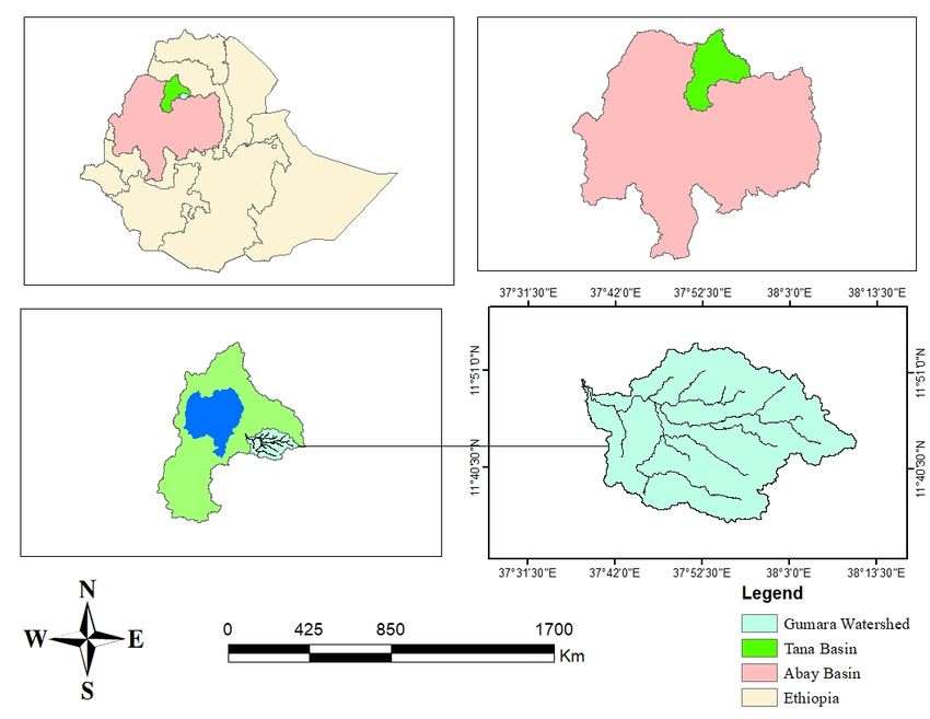
The Gumara River is located in Lake Tana basin and upper Blue Nile basin; it is located to the
east of the Lake Tana and extends between latitudes of 11◦ 350 and 11◦ 550 N and longitudes 37◦ 400 and
38◦ 100 E. The Gumara catchment has a total drainage area of 1271.86 km2 up to the gauging station
(near Woreta), 25 km before it joins the lake. The main stream starts from Guna Mountain; the total
length is 132.49 km (approximately) before it joins Lake Tana. According to [15] agro climate zone
classification, Gumara watershed is found in between Dega (cool and humid) and Woina Dega (cool
and sub humid) climate zones; the upper part of the catchment has Dega and the lower part has Woina
Dega climate zone condition, and the average annual rainfall is 1455.66mm (Figure 1).
2.2. Hydro-Climatic and Spatial Datasets
Historically, observed weather data of stations in and near the study area were collected from
NMA (National Meteorological Agency) of Ethiopia. The precipitation, maximum temperature,
and minimum temperature, which were basically needed for both climate and hydrological models,
were collected in five stations, whereas the other meteorological data like wind speed, relative humidity,
and sunshine hour were available in only two stations. As it is common in other parts of the country,
meteorological stations are sparsely distributed across the study area and not all stations have long-time
historical data. Climate model variables or predictors were obtained from the Canadian Climate data
and scenario website (http://climate-scenarios.canada.ca/?page=main).Water 2020, 12, 3046 3 of 14
Water 2020, 12, x FOR PEER REVIEW 3 of 15
Figure1.1.Location
Figure mapofofstudy
Location map studyarea.
area.
Recorded streamand
2.2. Hydro-Climatic flow dataDatasets
Spatial of Gumara River were collected from Ministry of Water Irrigation
and Energy (MoWIE) of Ethiopia. The time series of collected stream flow data was for the period of
Historically, observed weather data of stations in and near the study area were collected from
1985–2008 (24 years).
NMA (National Meteorological Agency) of Ethiopia. The precipitation, maximum temperature, and
Digital Elevation Model (DEM), Shuttle Radar Topography Mission (SRTM) (30m × 30m resolution),
minimum temperature, which were basically needed for both climate and hydrological models, were
and Land
collected in five data
use/cover werewhereas
stations, taken from USGS
the other Earth explorer
meteorological website
data (https://earthexplorer.usgs.gov/).
like wind speed, relative humidity,
The Land use coverage was extracted for the study area which has 73.33%
and sunshine hour were available in only two stations. As it is common in other Kappapartsstatistic and 88.33%
of the country,
overall classification
meteorological accuracy.
stations The other
are sparsely important
distributed acrossinput for flow
the study simulation
area and modelhave
not all stations waslong-
soil data
time from
obtained historical
the data. Climate
Ministry model variables
of Water, Irrigationorand
predictors
Energy were obtained
(MoWIE) offrom the Canadian Climate
Ethiopia.
data and scenario website (http://climate-scenarios.canada.ca/?page=main).
2.3. Data Recorded
Preparation and Bias
stream flowCorrection
data of Gumara River were collected from Ministry of Water Irrigation
and Energy (MoWIE) of Ethiopia. The time series of collected stream flow data was for the period of
Prior to analysis, the collected raw data were prepared to eliminate errors and biases. There
1985–2008 (24 years).
were some missing
Digital valuesModel
Elevation in all (DEM),
stationsShuttle
and these were
Radar replaced by
Topography −99, which
Mission is compatible
(SRTM)(30m × 30m for
SDSM model usedand
resolution), for climate projection,data
Land use/cover and for
werethe taken
SWAT model for simulation
from USGS of futurewebsite
Earth explorer stream flow.
The raw data were arranged in monthly
(https://earthexplorer.usgs.gov/). The Landbasis
useand stacked
coverage wasto daily annual
extracted time series
for the study basehas
area which so as to
make73.33%
it wellKappa
suitedstatistic and 88.33%
for climate overall
statistical classificationand
downscaling accuracy. The othersimulation
hydrological important input for flow
models.
simulation model
Predictor was soil
variables haddata
beenobtained from the
calibrated by Ministry
observedof Water,
stationIrrigation and Energy
data, which (MoWIE)to as
are referred
of Ethiopia.
predictands, through statistically adjusting the value of parameters. This statistical correlation of
parameters and predictands was done using SDSM model. This model has also produced the future
2.3. Data Preparation and Bias Correction
projected data of precipitation, maximum temperature, and minimum temperature of the stations based
Prior to analysis,
on the calibrated the collected
parameters. Both theraw data were prepared
temperature to eliminate
and rainfall changeerrors
wereand biases. There
evaluated were
comparatively
some missing values in all stations and these were replaced by −99, which is compatible for SDSM
between the historical data (1961–1990), which was considered as baseline data, and three future 30 year
model used for climate projection, and for the SWAT model for simulation of future stream flow. The
time series datasets, represented as 2020s (2011–2040), 2050s (2041–2070), and 2080s (2071–2100).Water 2020, 12, 3046 4 of 14
2.4. SWAT Model Setup, Calibration, and Validation
Like climate data, the raw data of stream flow had also been prepared to make it compatible
with the SWATCUP2012 software for calibration process. SWAT model passes the process through six
important steps in simulation of the stream flow. The six steps of modeling are (1) delineation of the
basin and river network extraction, (2) Hydrological Response Unit (HRU) definition and analysis,
(3) climate station and weather generation formation, (4) sensitivity analysis of parameters, (5) model
calibration, and (6) model validation.
The river network merged in to SRTM DEM using the “burn in” method, and the basin was
delineated into 24 sub basins. Sub basins of the catchment were further divided into 184 Hydrological
Response Units (HRUs) using the land use, soil and slope distribution process.
The observed 10 years of observed stream flow data (1985–1994) were used for model calibration;
and verification of calibrated parameters was tested by 1995–2000 (six) years of observed stream
flow data. The proportion of datasets used for calibration and validation of model parameters is
nearly similar with the recommended, which is that 70% of dataset should be taken for calibration
and 30% for validation [16]. The calibration process was carried out using SWATCUP2012 software.
Using this software, the calibration was run with 2000 iterations through automatically adjusting of
values of selected parameters within the range of adjustment domain. Sensitive parameters which
have significant influence on stream flow simulated by SWAT model were selected by the sensitivity
analysis process. Selected parameters are similar with the previous study done by [17]. The model
efficiency was evaluated by using statistical variables determining the fitness of simulated stream
flow with observed data. Those statistical variables, NS (Nash–Sutcliffe efficiency) and RVE (Relative
Volume Error), are shown in Equations (1) and Equation (2), respectively.
Pn 2
Qsim(i) − Qobs(i)
i=1
NS = 1 − P 2 (1)
n
i=1 Q sim ( i ) − Q obs
where Qobs and Qsim represent the observed and simulated daily stream flows, respectively, n refers to
the number of days in the simulated or observed time series period. The overbar symbol indicates the
mean value. The value of Nash–Sutcliffe efficiency (NS) ranges between 1 and −∞ 1; showing the best
fit of the model or that the model simulates similar values of stream flow with the observed values.
The value should be more than 0.5 to accept the model [18].
Pn
i=1 (Qsim(i) Qobs(i) )
RVE = Pn × 100% (2)
i=1 Qobs(i)
RVE indicates the ratios of the sum of differences in simulated and total observed value of stream
flow to the total observed stream flow.
2.5. Comparison of Stream Flow under RCP Scenarios
Once the model had been calibrated by selected parameters and validation was carried out for the
watershed, stream flow was simulated using those selected parameters and automatically adjusted
values of parameters. Stream flow was simulated using historical climate data and future projected
climate data under RCP2.6, RCP4.5, and RCP8.5 scenarios separately.
The impact of climate change on stream flow of the catchment under RCP2.6, RCP4.5, and RCP8.5
scenarios was evaluated by comparing the flow generated by projected climate data under those
scenarios in 2020s, 2050s, and 2080s with the baseline period (1961–1990). The land use characteristics
of the watershed is the other determinant factor for simulation of stream flow; but since the study
is designed to indentify the impact of climate change alone, the same land use cover data with the
baseline period was taken.RCP8.5 scenarios was evaluated by comparing the flow generated by projected climate data under
characteristics of the watershed is the other determinant factor for simulation of stream flow; but
those scenarios in 2020s, 2050s, and 2080s with the baseline period (1961–1990). The land use
since the study is designed to indentify the impact of climate change alone, the same land use cover
characteristics of the watershed is the other determinant factor for simulation of stream flow; but
data with the baseline period was taken.
since the study is designed to indentify the impact of climate change alone, the same land use cover
data
Water with12,the
3. Results
2020, andbaseline
3046 period was taken.
Discussion 5 of 14
3.3.1.
Results and Discussion
Simulation, Bias Correction,and Future Climate Data Projection
3. Results and Discussion
Statistically
3.1. Simulation, downscaled
Bias climate
Correction,and Future data were Data
Climate compared with the observed data. The efficiency of
Projection
3.1.
SDSMSimulation,
model Biaswas Correction,
evaluated,and
andFuture Climate Data
the difference Projection and observed maximum temperature
of simulated
Statistically downscaled climate data were compared with the observed data. The efficiency of
andStatistically
minimum downscaled
temperatureclimate
is shown inwere Figures 2 andwith 3, respectively.
observedThedata.difference between
SDSM model was evaluated, and thedata differencecompared
of simulated and the observed maximumThe efficiency
temperature of
observed
SDSM model andwassimulated
evaluated, maximum
and the temperature
difference of in the
simulatedbaseline
and period
observed is more
maximumprominent in
temperature theand
wet
and minimum temperature is shown in Figures 2 and 3, respectively. The difference between
season (June–September);
minimum temperature whereas the difference on the remaining months is insignificant. The
observed and simulatedismaximum
shown in Figures
temperature2 andin3,the
respectively. The difference
baseline period between
is more prominent observed
in the wet
maximum
and simulated variation
maximum is shown on June, which
temperature is 0.36 °C. The is
minimum temperature ofwet
downscaled
season (June–September); whereas theindifference
the baseline on period more prominent
the remaining months is in the season
insignificant. The
data showed
(June–September); positive difference
whereas the in all
differencemonths
on except
the August,
remaining October,
months is and November.
insignificant. The
The maximum
maximum
maximum variation is shown on June, which is 0.36 °C. The minimum temperature of downscaled
difference
variation is 0.32 °C,
is shown observed
on June, whichonisMarch shown
◦ C. in Figure 3.
data showed positive difference in all0.36
months The minimum
except August, temperature
October, and of November.
downscaledThedata showed
maximum
positive difference in all months except August,
difference is 0.32 °C, observed on March shown in Figure 3. October, and November. The maximum difference is
0.32 ◦ C, observed
0.8 on March shown in Figure 3.
Model
0.6
0.8
Model
0.4
0.6
Temperature
0.2
0.4
(oC) (oC)
Temperature
0.0
0.2
ErrorError
-0.2
0.0
Maximum
-0.4
-0.2
Maximum
-0.6
-0.4
Jan Feb Mar Apr May Jun Jul Aug Sep Oct Nov Dec
-0.6
Jan Feb Mar Apr May Jun Jul Aug Sep Oct Nov Dec
Figure 2. CanESM2 model error of maximum temperature for the baseline period (1961–1990).
Figure 2. CanESM2 model error of maximum temperature for the baseline period (1961–1990).
Figure 2. CanESM2 model error of maximum temperature for the baseline period (1961–1990).
0.8
0.6
Temperature
0.8
(oC) (oC)
0.4
0.6
Temperature
Model Error
0.2
0.4
Error
0.0
0.2
Minimum
-0.2
0.0
Minimum
Model
-0.4
-0.2
-0.6
-0.4
Jan Feb Mar Apr May Jun Jul Aug Sep Oct Nov Dec
-0.6
Jan Feb
Figure 3. CanESM2 Mar
model error Apr May temperature
of minimum Jun Jul forAug Sep period
the baseline Oct (1961–1990).
Nov Dec
Figure 3. CanESM2 model error of minimum temperature for the baseline period (1961–1990).
The model cannot reasonably capture the observed rainfall of the baseline period in rainy season
Figure 3. CanESM2 model error of minimum temperature for the baseline period (1961–1990).
(June–September). Indeed, the change is significant in summer (rainy) season because rain is not
common in the winter seasons in the study area. The change is negative at the beginning of the rainy
season, and it is positive in the last two months of the summer season. The overall average difference
between observed and downscaled rainfall data of the study area is 0.58 mm/day shown in Figure 4.
Statistical Down Scaling Model (SDSM) for CanESM2 climate model in RCP scenarios has been used
by other researchers in the region and it has good fitness with the real data [19].common in the winter seasons in the study area. The change is negative at the beginning of the rainy
season, and it is positive in the last two months of the summer season. The overall average difference
between observed and downscaled rainfall data of the study area is 0.58 mm/day shown in Figure 4.
Statistical Down Scaling Model (SDSM) for CanESM2 climate model in RCP scenarios has been used
by other
Water researchers
2020, 12, 3046 in the region and it has good fitness with the real data [19]. 6 of 14
3.0
Rainfall Model Error
2.0
(mm/day)
1.0
0.0
-1.0
-2.0
-3.0
Jan Feb Mar Apr May Jun Jul Aug Sep Oct Nov Dec
Figure4.4.Model
Figure Modelerror
errorofofrainfall
rainfallbetween
betweenobserved
observedand
anddownscaled
downscaleddata
dataofofthe
thebaseline
baselineperiod
period(1961–1990).
(1961–
1990).
3.2. Calibration and Validation of SWAT Model
3.2. The
Calibration
streamandflowValidation of SWAT Model
of the watershed was simulated using the SWAT hydrological model. Based
on the sensitivity analysis which was conducted to determine parameters affecting the stream flow;
The stream flow of the watershed was simulated using the SWAT hydrological model. Based on
11 sensitive parameters were selected. Among these sensitive parameters, V_ALPHA_BF (base flow),
the sensitivity analysis which was conducted to determine parameters affecting the stream flow; 11
and CN2 (curve number) were found to be the most sensitive parameters. The calibration process
sensitive parameters were selected. Among these sensitive parameters, V_ALPHA_BF (base flow),
was carried out using the SWATCUP2012 software. The model was calibrated by model parameters,
and CN2 (curve number) were found to be the most sensitive parameters. The calibration process
and those parameters with fixed value have also been validated. The efficiency was measured by NS
was carried out using the SWATCUP2012 software. The model was calibrated by model parameters,
and RVE, and the values of those statistical variables are 0.66% and 0.72%, respectively. This fitness
and those parameters with fixed value have also been validated. The efficiency was measured by NS
was also verified and it gives NS (0.63) and RVE (1.24%). Thus, based on the values of those efficiency
and RVE, and the values of those statistical variables are 0.66 and 0.72%, respectively. This fitness
determinant variables, the model showed consistency with those optimized values of parameters on
was also verified and it gives NS (0.63) and RVE (1.24%). Thus, based on the values of those efficiency
the study
Water
area andPEER
2020, 12, x FOR
it is possible to say that these parameter values are representative of the Gumara
determinant variables,REVIEW
the model showed consistency with those optimized values of parameters 7 of 15
on
watershed (Figure 5).
the study area and it is possible to say that these parameter values are representative of the Gumara
watershed (Figure 5).
Observed Flow Simulated Flow Rainfall
480 0
400 50
320 100
Flow (m3/s)
Rainfall (mm/day)
240 150
160 200
80 250
0 300
Figure 5. Comparison of simulated and observed flow for the calibration period (1985–1994).
Figure 5. Comparison of simulated and observed flow for the calibration period (1985–1994).
The simulation flow in calibration period captures the peak flow in some years and it follows
similar patterns, although in some years the simulated peak flow is above the peak values of observed
The simulation flow in calibration period captures the peak flow in some years and it follows
stream flow and vice versa. In dry season, the simulated flow did not best captured the line; there
similar patterns, although in some years the simulated peak flow is above the peak values of observed
is a light shifting to the right which shows that it is a little bit overestimated. In the calibration
stream flow and vice versa. In dry season, the simulated flow did not best captured the line; there is
process, the model had good efficiency and the simulated flow closely followed the pattern of observed
a light shifting to the right which shows that it is a little bit overestimated. In the calibration process,
stream flow. Only three meteorological stations were used to represent the basin for this study; one
the model had good efficiency and the simulated flow closely followed the pattern of observed stream
flow. Only three meteorological stations were used to represent the basin for this study; one of which
is located out of the watershed, and the altitudinal variation of the study area is also very high. For
this reason, the rainfall is extremely variable in terms of the spatial distribution within this area
[20,21], and the rainfall data used for the study may not be fully representative of the entire
watershed. Therefore, this may have increased the spatial variability of runoff in the catchment, andThe simulation flow in calibration period captures the peak flow in some years and it follows
similar patterns, although in some years the simulated peak flow is above the peak values of observed
stream flow and vice versa. In dry season, the simulated flow did not best captured the line; there is
a light shifting to the right which shows that it is a little bit overestimated. In the calibration process,
Water 2020, 12, 3046 7 of 14
the model had good efficiency and the simulated flow closely followed the pattern of observed stream
flow. Only three meteorological stations were used to represent the basin for this study; one of which
is
oflocated
which is out of the out
located watershed, and the altitudinal
of the watershed, variation of
and the altitudinal the study
variation of area is alsoarea
the study veryis high. For
also very
this
high.reason,
For this the rainfall
reason, theisrainfall
extremely variable variable
is extremely in termsinofterms
the spatial distribution
of the spatial withinwithin
distribution this area
this
[20,21], and the rainfall data used for the study may not be fully representative
area [20,21], and the rainfall data used for the study may not be fully representative of the entire of the entire
watershed.
watershed. Therefore,
Therefore,this
thismay
mayhave
haveincreased
increasedthethespatial
spatialvariability
variabilityof ofrunoff
runoff inin the
the catchment,
catchment, andand
hence
hence some
some variations
variations in
in peak
peak flows
flows ofof the
the simulated
simulated and
and observed
observed flow
flow were
were shown.
shown.
The calibratedparameters
The calibrated parametersof ofthethe study
study area been
area have haveverified
been verified
to measureto measure
their leveltheir level of
of consistency
consistency by using six years of meteorological data (1995–2000). The simulated
by using six years of meteorological data (1995–2000). The simulated flow reasonably captured the flow reasonably
captured
peaks butthe alsopeaks but also
showed modestshowed modest
variation variation
in dry seasonin dry season
flows (Figureflows
6). (Figure 6).
400
300
Flow (m3/s)
200
100
0
1995/1/1 1996/1/1 1997/1/1 1998/1/1 1999/1/1 2000/1/1
Observed Flow Simulated Flow
Figure 6. Comparison of simulated flow and observed flow for the validation period (1995–2000).
Figure 6. Comparison of simulated flow and observed flow for the validation period (1995–2000).
3.3. Changes of Climate under RCP Scenarios
The change of rainfall, maximum temperature, and minimum temperature based on RCP2.6,
RCP4.5, and RCP 8.5 scenarios were analyzed in terms of monthly basis, because it is designed to
reveal seasonal variation. The change was shown between the three phases of the whole period (2020s,
2050s, and 2070s) in which thirty years of time series is contained, compared with the baseline period
(1961–1990).
3.3.1. Change in Rainfall
The average monthly rainfall in the study area for the whole period of this century has been
forecasted under RCP 2.6, RCP 4.5, and RCP 8.5 climate scenarios. Under RCP 2.6 scenario, the maximum
change of monthly average rainfall shows an increment of 38.21% in October and the minimum change
is −2.30% in November by 2080s period, and the variability of changes observed within this range is
shown in Figure 7. Under this climate scenario, almost all months, except two consecutive months
(January and February), it is shown an increase in rainfall amount. The rainfall change under RCP
4.5 scenario ranges from 0.61% to 42.11% in both increasing and decreasing values, where the minimum
value is observed in March within 2080s, and the maximum change is also in February but in the
middle of 21st century (2050s), shown in Figure 8. In RCP 4.5 scenario, there is an increment in three
consecutive months (August–November), whereas in the remaining months (e.g., December, May,
June, and July) the change is not considerable. Like in RCP 4.5, the rainfall trend in RCP 8.5 exhibited
a similar pattern, namely a fluctuating pattern in monthly bases even though both the upward and
downward maximum change is relatively small compared with that of the RCP 4.5. The range of
change is between 0.64% and 33.08% in increasing and decreasing values. The maximum change is
observed in February within 2080s, shown in Figure 9. Even though different models were used, the
result of this study is consistent with the findings of other studies near to Gumara watershed [22,23],
and out of the region [24]. Moreover, the change in annual average rainfall in percent for the future
time periods was found to be increasing for all scenarios, but when we compare the change betweenincrement in three consecutive months (August–November), whereas in the remaining months (e.g.,
December, May, June, and July) the change is not considerable. Like in RCP 4.5, the rainfall trend in
RCP 8.5 exhibited a similar pattern, namely a fluctuating pattern in monthly bases even though both
the upward and downward maximum change is relatively small compared with that of the RCP 4.5.
The range of change is between 0.64% and 33.08% in increasing and decreasing values. The maximum
change is observed in February within 2080s, shown in Figure 9. Even though different models were
Water 2020, 12, 3046 8 of 14
used, the result of this study is consistent with the findings of other studies near to Gumara watershed
[22,23], and out of the region [24]. Moreover, the change in annual average rainfall in percent for the
future time periods was found to be increasing for all scenarios, but when we compare the change
the three scenarios, the variation is not that considerable. Similar observations have been made in
between the three scenarios, the variation is not that considerable. Similar observations have been
other parts
madeofinthe world
other parts[25].
of the world [25].
RCP 2.6
50
40
30
Change in Rainfall (%)
20
10
0
-10
-20
2020S
-30
-40 2050S
-50
Jan Feb Mar Apr May Jun Jul Aug Sep Oct Nov Dec 2080S
Figure
Water7. Change
Figure
2020, 12, 7. in PEER
rainfall
Change
x FOR in under
rainfall Representative
REVIEW Concentration
under Representative Pathway
Concentration (RCP2.6)
Pathway scenario
(RCP2.6) compared
scenario9 of 15
Water 2020, 12, x FOR PEER REVIEW 9 of 15
compared to the
to the baseline (1961–1990). baseline (1961–1990).
50 RCP 4.5
50 RCP 4.5
40
40
30
(%)
30
(%)
20
Rainfall
20
Rainfall
10
10
0
0
inin
-10
Change
-10
Change
-20
-20
-30
-30
-40 2020s
-40 2020s
-50
-50 2050s
Jan Feb Mar Apr May Jun Jul Aug Sep Oct Nov Dec 2050s
Jan Feb Mar Apr May Jun Jul Aug Sep Oct Nov Dec 2080s
2080s
Figure 8. Change in rainfall under RCP4.5 scenario compared to the baseline (1961–1990).
8. Change
FigureFigure in rainfall
8. Change under
in rainfall underRCP4.5
RCP4.5 scenario compared
scenario compared to the
to the baseline
baseline (1961–1990).
(1961–1990).
50 RCP 8.5
50 RCP 8.5
40
40
(%)
30
(%)
30
20
Rainfall
20
Rainfall
10
10
0
0
inin
-10
Change
-10
-20
Change
-20
-30
-30
-40 2020s
-40 2020s
-50 2050s
-50 2050s
Jan Feb Mar Apr May Jun Jul Aug Sep Oct Nov Dec 2080s
Jan Feb Mar Apr May Jun Jul Aug Sep Oct Nov Dec 2080s
9. Change
Figure Figure in rainfall
9. Change under
in rainfall RCP8.5
under RCP8.5 scenarios compared
scenarios compared to the
to the baseline
baseline (1961–1990).
(1961–1990).
Figure 9. Change in rainfall under RCP8.5 scenarios compared to the baseline (1961–1990).
3.3.2. Change in Maximum and Minimum Temperature
3.3.2. Change in Maximum and Minimum Temperature
In this study, the change in the projected maximum temperature and minimum temperature of
In this study, the change in the projected maximum temperature and minimum temperature of
the three time frames compared to the baseline (1961–1990) period in all RCP scenarios was revealed.
the three time frames compared to the baseline (1961–1990) period in all RCP scenarios was revealed.
The change of maximum temperature in monthly average basis under the RCP 2.6 scenario varies
The change of maximum temperature in monthly average basis under the RCP 2.6 scenario varies
between 0.26 °C and 1.66 °C in 2020s and 2080s, respectively, as shown in Figure 10. In this scenario,
between 0.26 °C and 1.66 °C in 2020s and 2080s, respectively, as shown in Figure 10. In this scenario,
the maximum change in minimum temperature is 1.19 °C, which is observed in October 2080s. In
the maximum change in minimum temperature is 1.19 °C, which is observed in October 2080s. InWater 2020, 12, 3046 9 of 14
3.3.2. Change in Maximum and Minimum Temperature
In this study, the change in the projected maximum temperature and minimum temperature of
the three time frames compared to the baseline (1961–1990) period in all RCP scenarios was revealed.
The change of maximum temperature in monthly average basis under the RCP 2.6 scenario varies
between 0.26 ◦ C and 1.66 ◦ C in 2020s and 2080s, respectively, as shown in Figure 10. In this scenario,
the maximum change in minimum temperature is 1.19 ◦ C, which is observed in October 2080s. In RCP
4.5 scenario, the change in monthly average maximum temperature ranges from 0.51 ◦ C (December)
to 3.38 ◦ C (July), shown in Figure 10. The change in average maximum temperature at the end
of this century under RCP 4.5 and RCP 8.5 scenarios is 2.6 ◦ C and 3.8 ◦ C, respectively, shown in
Figure 11. The change in monthly average minimum temperature under RCP 4.5 also ranges from
0.14 ◦ C (August) to 2.67 ◦ C (October), shown in Figure 12. Under RCP 4.5 and RCP 8.5 scenarios, the
change in average minimum temperature is found to be increasing by 1.69 ◦ C and 4.02 ◦ C, respectively
(Figure 13). The change in both maximum temperature and minimum temperature under RCP 8.5 was
found to be increasing prominently compared with the other scenarios; the change in monthly average
maximum temperature ranges from 0.42 ◦ C in August to 4.96 ◦ C in April, shown in (Figure 10). Climate
Water 2020,in
Scenarios 12,RCP
x FOR 2.6,
PEERRCP
REVIEW
4.5, and RCP 8.5 are developed with assumptions of having 2.6 10 of 15 2 ,
W/m
4.5 W/m2 , and 8.5 W/m2 radiative forcing, respectively. Because of these concentrations of radiative
of having 2.6 W/m2, 4.5 W/m2, and 8.5 W/m2 radiative forcing, respectively. Because of these
forces, these scenarios are also assumed to be the cause for the change in average temperature by 1.5 ◦ C
concentrations of radiative forces, these scenarios are also assumed to be the cause for the change in
(RCP2.6), 2.4 ◦ C (RCP4.5), and 4.9 ◦ C (RCP8.5) [26], and the results of this study are consistent with
average temperature by 1.5 °C (RCP2.6), 2.4 °C (RCP4.5), and 4.9 °C (RCP8.5) [26], and the results of
this assumption. Moreover, the result of this study regarding the change in maximum and minimum
this study are consistent with this assumption. Moreover, the result of this study regarding the
temperature matches with that of other previous studies [27] near to the study area, and [28,29] out of
change in maximum and minimum temperature matches with that of other previous studies [27] near
the
toregion.
the study area, and [28,29] out of the region.
6
Change in Maximum Temperature (OC)
5
4
3
2
1
0
Jan Feb Mar Apr May Jun Jul Aug Sep Oct Nov Dec
RCP 2.6_2020s RCP 2.6_2050s RCP 2.6_2080s RCP4.5_2020s RCP4.5_2050s
RCP4.5_2080s RCP8.5_2020s RCP8.5_2050s RCP8.5_2080s
Figure10.
Figure 10. Change
Changeininmonthly
monthlyaverage maximum
average temperature
maximum compared
temperature to the baseline
compared to the period (1961–
baseline period
1990).
(1961–1990).
4
hange in Average Maximum
3.5
3
Temperature (OC)
2.5
2
1.5
1
0.5RCP 2.6_2020s RCP 2.6_2050s RCP 2.6_2080s RCP4.5_2020s RCP4.5_2050s
RCP4.5_2080s RCP8.5_2020s RCP8.5_2050s RCP8.5_2080s
Water 2020, 12, Figure
3046 10. Change in monthly average maximum temperature compared to the baseline period (1961– 10 of 14
1990).
4
Change in Average Maximum
3.5
3
Temperature (OC) 2.5
2
1.5
1
0.5
0
Figure 11. Change inxannual
Water 2020, 12, FOR PEER average
REVIEW
Water 2020, 12, x FOR PEER REVIEW
maximum temperature compared to baseline period
11 of 15(1961–1990).
11 of 15
Figure 11. Change in annual average maximum temperature compared to baseline period (1961–
7
1990). 7
OC)
Temperature(O(C)
6
6
MinimumTemperature
5
5
4
4
ChangeininMinimum
3
3
2
2
Change
1
1
0
0
Jan Feb Mar Apr May Jun Jul Aug Sep Oct Nov Dec
Jan Feb Mar Apr May Jun Jul Aug Sep Oct Nov Dec
RCP2.6_2020s RCP2.6_2050s RCP2.6_2080s RCP4.5_2020s RCP4.5_2050s
RCP2.6_2020s RCP2.6_2050s RCP2.6_2080s RCP4.5_2020s RCP4.5_2050s
RCP4.5_2080s RCP8.5_2020s RCP8.5_2050s RCP8.5_2080s
RCP4.5_2080s RCP8.5_2020s RCP8.5_2050s RCP8.5_2080s
Figure 12.
Figure 12. Change inChange in monthly
monthly average maximum
average minimum temperature compared tocompared
temperature the baseline period (1961–baseline period
to the
Figure 12. Change in monthly average maximum temperature compared to the baseline period (1961–
1990).
(1961–1990). 1990).
4.5
Temperature
4.5
MinimumTemperature
4
4
3.5
3.5
3
3
AverageMinimum
2.5
2.5
OC)
(O(C)
2
2
ChangeininAverage
1.5
1.5
1
1
0.5
0.5
Change
0
0
Figure 13. Change in annual average minimum temperature compared to the baseline period
Figure 13. Change in annual average minimum temperature compared to the baseline period (1996–
(1996–1990). 1990).
Figure 13. Change in annual average minimum temperature compared to the baseline period (1996–
1990).3.4. Evaluating Impact of Climate Change on Stream Flow
The change in stream flow of Gumara watershed under RCP 2.6, RCP 4.5, and RCP 8.5 scenarios
shows an increasing trend in monthly average values in some months and years, but a decreasing
Water
trend2020, 12, 3046
is also observed in some years of the studied period. In RCP 2.6 scenario, the change in stream 11 of 14
flow was found to be increasing in almost all months other than January and February with some
exceptions in 2080s, shown in Figure 14. The change under this scenario ranges from 1.11% in July
3.4. Evaluating Impact of Climate Change on Stream Flow
2020s to 19.18% in August 2080s. In RCP 2.6 scenario, the average stream flow recorded an increment
The in
of 4.43% change
2020s,in3.09%
stream in flow
2050s, ofand
Gumara3.29%watershed
in 2080s; but under
the RCP
change 2.6,isRCP 4.5, and
decreased RCP 8.5these
between scenarios
three
shows an increasing trend in monthly average values in some
time frames. However, when considered on a monthly basis, the change in stream flow shows months and years, but a decreasing
trend is alsoincrease
consistent observed underin someRCPyears of the studied
4.5 scenario. period. In
For example, theRCP 2.6 scenario,
stream flow change the change
increases in stream
in five
flow
consecutive months (July–November), whereas in the other months it shows decreasing with a some
was found to be increasing in almost all months other than January and February with small
exceptions
exception ininMay, 2080s, shown
shown in in Figure15).
(Figure 14.The
Thechange
changerangesunderfrom this scenario
1.21% in ranges from 1.11%
May (period) in July
to 20.97% in
2020s
August to 19.18%
(2080s).inDue August 2080s.
to this, theInlocal
RCP farmers
2.6 scenario,
will thenotaverage stream flow
have adequate waterrecorded an increment
for their irrigation
of 4.43% in 2020s,
agriculture; because 3.09%
they in 2050s,
have beenand 3.29% intheir
cultivating 2080s; butthrough
land the change is decreased
diverting the dry between
season streamthese
three time frames. However, when considered on a monthly basis,
flow of Gumara River. Even though there is high variability between months, in RCP 4.5 scenario, the change in stream flow shows
consistent
the changeincrease
in averageunder streamRCPflow 4.5 scenario. For example,
is not considerable; it is the stream
2.21%, flow
2.45%, andchange
2.53%increases
in 2020s,in five
2050s,
consecutive months (July–November), whereas in the other months
and 2080s, respectively. Under RCP 8.5 scenario, the change in stream flow indicates insignificant it shows decreasing with a small
exception
increase inin dryMay, shown
seasons butinit (Figure 15). The
is decreasing change
in the ranges (rainy
pre summer from 1.21%
season),in May
shown (period)
in Figureto 16.
20.97%
The
in August (2080s). Due to this, the local farmers will not have
change in stream flow under all scenarios shows significant increase in summer and post summer adequate water for their irrigation
agriculture;
(October and because they have
November) been cultivating
seasons, but in dry theirseason
land through
due todiverting the dryinseason
the increase stream
temperature
flow of Gumara River.
evapotranspiration will Evenbe though
increased there is high
[30], andvariability
consequently betweenthe months,
catchment in RCP
may4.5 bescenario,
exposedthe to
change in average stream flow is not considerable; it is 2.21%,
seasonal moisture deficit [31]. Moreover the average stream flow change in RCP 8.5 scenario is2.45%, and 2.53% in 2020s, 2050s, and
2080s, respectively.
indicating Underand
4.06%, 3.26%, RCP 8.5 scenario,
3.67% in 2020s,the change
2050s, andin2080s,
streamrespectively.
flow indicates The insignificant
result of this increase
study
in dry seasons
showed somehow but itconsistency
is decreasing in the
with pre summer
previous results(rainy season),works
of research shownconducted
in Figure 16.usingThedifferent
change
in stream
climate flow under
models all scenarios
and scenarios in theshows
adjacentsignificant
watersheds increase in summer and post summer (October
[27,32,33].
and November)
The changeseasons,
in temperaturebut in dry andseason
rainfalldue
willto disturb
the increase in temperature
the integrity evapotranspiration
of the whole ecosystems ofwill the
be increased [30], and consequently the catchment may be exposed to
watershed, including the water ecosystems of lake Tana; and all its ecosystem services [34]. Therefore, seasonal moisture deficit [31].
Moreover
physical soil theand
average
waterstream flow change
conservation in RCPmanagement)
(watershed 8.5 scenario is indicating
practices and4.06%, 3.26%,
biological and 3.67%
conservation
in 2020s, 2050s,
methods and 2080s, respectively.
like afforestation and preserving Thetheresult of this
natural study showed
environment [35]somehow
should beconsistency
executed onwith the
previous results of research works conducted using different climate
upper catchment of the study area to reduce the impact of climate change, like flooding and sediment models and scenarios in the
adjacent
transportwatersheds
to the lake [27,32,33].
during rainy season and hydrological drought in dry season.
RCP 2.6
25
20
15
Change in flow (%)
10
5
0
-5
-10 2020s
-15 2050s
Jan Feb Mar Apr May Jun Jul Aug Sep Oct Nov Dec 2080s
Figure 14. Change
Figure 14. Changeininstream
streamflow under
flow RCP
under 2.6 2.6
RCP scenario compared
scenario to the
compared tobaseline period
the baseline (1961–1990).
period (1961–
1990).Water 2020, 12, 3046 12 of 14
Water 2020, 12, x FOR PEER REVIEW 13 of 15
25
RCP 4.5
Change in Flow (%) 20
15
10
5
0
-5
-10 2020s
-15 2050s
Jan Feb Mar Apr May Jun Jul Aug Sep Oct Nov Dec 2080s
Figure
Figure 15. Change
15. Change in stream
in stream flowunder
flow underRCP4.5
RCP4.5 scenario
scenariocompared
comparedto to
thethe
baseline period
baseline (1961–1990).
period (1961–1990).
RCP 8.5
25
20
Change in Flow (%)
15
10
5
0
-5
-10 2020s
-15 2050s
Jan Feb Mar Apr May Jun Jul Aug Sep Oct Nov Dec
2080s
Figure 16. Change
Figure in stream
16. Change flowflow
in stream under RCP
under 8.5 8.5
RCP scenarios compared
scenarios toto
compared the baseline
the baselineperiod
period(1961–1990).
(1961–
1990).
The change in temperature and rainfall will disturb the integrity of the whole ecosystems of the
4. Conclusions
watershed, including the water ecosystems of lake Tana; and all its ecosystem services [34]. Therefore,
physical soil
The and water
future conservation
climate (watershed
and its impact on the management) practices
stream flow under and biological
Representative conservation
Concentration
methods like scenarios
Pathway afforestation
in theand
subpreserving the Blue
basin of Upper natural
Nileenvironment
basin (Gumara[35] should be
watershed) executed
were on the
evaluated
upperusing
catchment
CanESM2 of the study
climate areaand
model to reduce the impact
statistically of climate
downscaling change,
model. Streamlike flooding
flow and sediment
of the study area
was simulated
transport to the lakebyduring
using SWAT model.and
rainy season The hydrological
findings revealed that in
drought there
dryisseason.
an increment in both
maximum and minimum temperature under all scenarios in 2020s, 2050s, and 2080s with a higher
4. Conclusions
rate of increase towards the end of the century. This leads toan increase in evapotranspiration and
loss of moisture in the catchment. Even though there is no significant difference in the range and
The future climate and its impact on the stream flow under Representative Concentration Pathway
average change in rainfall between the three scenarios, the range of change in monthly average
scenarios in the
rainfall sub basinhigher
is somewhat of Upper Blue
under Nile
RCP 2.6basin (Gumara
scenario watershed)
than in were evaluated
other scenarios. The change using CanESM2
in stream
climate
flow of Gumara watershed under RCP 2.6, RCP 4.5, and RCP 8.5 scenarios shows increasing trend in by
model and statistically downscaling model. Stream flow of the study area was simulated
usingmonthly
SWAT model.
average The findings
values in somerevealed thatyears,
months and there but
is an increment
decreasing in both
trend maximum
was also observed and minimum
in some
years of the
temperature studied
under period. Overall,
all scenarios the results
in 2020s, 2050s,ofand
this2080s
study with
suggest that therate
a higher change in climatetowards
of increase under the
RCP
end of the2.6, RCP4.5,
century. andleads
This RCP8.5
toanscenarios has
increase inaevapotranspiration
strong bearing on theand
rateloss
of the
of annual
moistureaverage
in thestream
catchment.
flow, which increased by 4.06%, 3.26%, and 3.67%, respectively. Watershed management
Even though there is no significant difference in the range and average change in rainfall between practices
the three scenarios, the range of change in monthly average rainfall is somewhat higher under RCP
2.6 scenario than in other scenarios. The change in stream flow of Gumara watershed under RCP 2.6,
RCP 4.5, and RCP 8.5 scenarios shows increasing trend in monthly average values in some months andWater 2020, 12, 3046 13 of 14
years, but decreasing trend was also observed in some years of the studied period. Overall, the results
of this study suggest that the change in climate under RCP 2.6, RCP4.5, and RCP8.5 scenarios has a
strong bearing on the rate of the annual average stream flow, which increased by 4.06%, 3.26%, and
3.67%, respectively. Watershed management practices and preservation of natural environment should
be done to mitigate the risk of climate change on the hydrological dynamics of the watershed.
Author Contributions: G.G.C. designed the hydrological model calibration and validation, downscaling of
climate data, and writing of the paper. S.S. and T.Z. supervised the research and edited the paper. All authors
have read and agreed to the published version of the manuscript.
Funding: This research was funded by EFOP-3.6.1-16-2016-00022 “Debrecen Venture Catapult program”.
The project is co-financed by the European Union and the European Social Fund.
Acknowledgments: We would like to thank National Meteorological Agency of Ethiopia (NMA), and Ministry of
Water Irrigation and Energy (MoWIE) of Ethiopia for providing free input data for this research work. This paper
is part of a PhD research project of the first author (G.G.C.) funded by the Tempus Public Foundation (Hungary)
within the framework of the Stipendium Hungaricum Scholarship Programme, supported by Ministry of Science
and Higher Education (MoSHE) of Ethiopia and Debark University.
Conflicts of Interest: The authors declare no conflict of interest.
References
1. Pachauri, R.K.; Allen, M.R.; Barros, V.R.; Broome, J.; Cramer, W.; Christ, R.; Church, J.A.; Clarke, L.; Dahe, Q.;
Dasgupta, P. Climate Change 2014: Synthesis Report. Contribution of Working Groups I, II and III to the Fifth
Assessment Report of the Intergovernmental Panel on Climate Change; IPCC: Geneva, Switzerland, 2014.
2. Hofmann, D.J.; Butler, J.H.; Dlugokencky, E.J.; Elkins, J.W.; Masarie, K.; Montzka, S.A.; Tans, P. The role of
carbon dioxide in climate forcing from 1979 to 2004: Introduction of the Annual Greenhouse Gas Index.
Tellus B Chem. Phys. Meteorol. 2006, 58, 614–619. [CrossRef]
3. Adopted, I. Climate Change 2014 Synthesis Report; IPCC: Geneva, Szwitzerland, 2014.
4. Hegerl, G.C.; Hoegh-Guldberg, O.; Casassa, G.; Hoerling, M.P.; Kovats, R.; Parmesan, C.; Pierce, D.W.;
Stott, P.A. Good practice guidance paper on detection and attribution related to anthropogenic climate
change. In Meeting Report of the Intergovernmental Panel on Climate Change Expert Meeting on Detection and
Attribution of Anthropogenic Climate Change; IPCC Working Group I Technical Support Unit, University of
Bern: Bern, Switzerland, 2010.
5. Tadege, A. Climate Change National Adaptation Program of Action (NAPA) of Ethiopia; National Meteorological
Agency: Addis Ababa, Ethiopia, 2007.
6. Cheung, W.H.; Senay, G.B.; Singh, A. Trends and spatial distribution of annual and seasonal rainfall in
Ethiopia. Int. J. Climatol. A J. R. Meteorol. Soc. 2008, 28, 1723–1734. [CrossRef]
7. EEA, J. WHO (2008): Impacts of Europe’s Changing Climate-2008 Indicator-Based Assessment; European
Environment Agency: Copenhagen, Denmark, 2008.
8. Bekele, L. Indications of the changing nature of rainfall in Ethiopia: The example of the 1st decade of 21st
century. Afr. J. Environ. Sci. Technol. 2015, 9, 104–110.
9. Haile, A.T.; Akawka, A.L.; Berhanu, B.; Rientjes, T. Changes in water availability in the Upper Blue Nile basin
under the representative concentration pathways scenario. Hydrol. Sci. J. 2017, 62, 2139–2149. [CrossRef]
10. Arnell, N.W. Climate change and global water resources. Glob. Environ. Chang. 1999, 9, S31–S49. [CrossRef]
11. Arnell, N.W. Climate change and global water resources: SRES emissions and socio-economic scenarios.
Glob. Environ. Chang. 2004, 14, 31–52. [CrossRef]
12. Shiklomanov, I. Comprehensive Assessment of the Freshwater Resources and Water Availability in the World:
Assessment of Water Resources and Water Availability in the World; World Meteorological Organization: Geneva,
Switzerland, 1997.
13. Worqlul, A.W.; Dile, Y.T.; Ayana, E.K.; Jeong, J.; Adem, A.A.; Gerik, T. Impact of climate change on streamflow
hydrology in headwater catchments of the Upper Blue Nile Basin, Ethiopia. Water 2018, 10, 120. [CrossRef]
14. Dile, Y.T.; Berndtsson, R.; Setegn, S.G. Hydrological response to climate change for gilgel abay river, in the
lake tana basin-upper blue Nile basin of Ethiopia. PLoS ONE 2013, 8, e79296. [CrossRef] [PubMed]
15. Hurni, H. Agroecological belts of Ethiopia.Explanatory Notes on Three Maps at a Scale of 1:1,000,000; Wittwer
Druck AG: Bern, Switzerland, 1998.Water 2020, 12, 3046 14 of 14
16. Klemeš, V. Operational testing of hydrological simulation models. Hydrol. Sci. J. 1986, 31, 13–24. [CrossRef]
17. Chakilu, G.; Moges, M. Assessing the land use/cover dynamics and its impact on the low flow of Gumara
watershed, Upper Blue Nile Basin, Ethiopia. Hydrol. Curr. Res. 2017, 8, 1–6. [CrossRef]
18. Nash, J.E.; Sutcliffe, J.V. River flow forecasting through conceptual models part I—A discussion of principles.
J. Hydrol. 1970, 10, 282–290. [CrossRef]
19. Fenta Mekonnen, D.; Disse, M. Analyzing the future climate change of Upper Blue Nile River basin using
statistical downscaling techniques. Hydrol. Earth Syst. Sci. 2018, 22, 2391–2408. [CrossRef]
20. Tilahun, K. Analysis of rainfall climate and evapo-transpiration in arid and semi-arid regions of Ethiopia
using data over the last half a century. J. Arid Environ. 2006, 64, 474–487. [CrossRef]
21. Worqlul, A.W.; Yen, H.; Collick, A.S.; Tilahun, S.A.; Langan, S.; Steenhuis, T.S. Evaluation of CFSR, TMPA
3B42 and ground-based rainfall data as input for hydrological models, in data-scarce regions: The upper
Blue Nile Basin, Ethiopia. Catena 2017, 152, 242–251. [CrossRef]
22. Taye, M.T.; Ntegeka, V.; Ogiramoi, N.; Willems, P. Assessment of climate change impact on hydrological
extremes in two source regions of the Nile River Basin. Hydrol. Earth Syst. Sci. 2011, 15, 209. [CrossRef]
23. Seleshi, Y.; Zanke, U. Recent changes in rainfall and rainy days in Ethiopia. Int. J. Climatol. A J. R. Meteorol. Soc.
2004, 24, 973–983. [CrossRef]
24. Tahir, T.; Hashim, A.; Yusof, K. Statistical downscaling of rainfall under transitional climate in Limbang
River Basin by using SDSM. In IOP Conference Series: Earth and Environmental Science; IOP Conference Series:
Langkawi, Malaysia, 2018.
25. Phinzi, K.; Ngetar, N.S. Land use/land cover dynamics and soil erosion in the Umzintlava catchment (T32E),
Eastern Cape, South Africa. Trans. R. Soc. S. Afr. 2019, 74, 223–237. [CrossRef]
26. Wayne, G. The beginner’s guide to representative concentration pathways. Skept. Sci. 2013, 3, 25.
27. Kim, U.; Kaluarachchi, J.J.; Smakhtin, V.U. Climate Change Impacts on Hydrology and Water Resources of the
Upper Blue Nile River Basin, Ethiopia; IWMI: Colombo, Sri Lanka, 2008; Volume 126.
28. Tan, M.L.; Yusop, Z.; Chua, V.P.; Chan, N.W. Climate change impacts under CMIP5 RCP scenarios on water
resources of the Kelantan River Basin, Malaysia. Atmos. Res. 2017, 189, 1–10. [CrossRef]
29. Mishra, V.; Lilhare, R. Hydrologic sensitivity of Indian sub-continental river basins to climate change.
Glob. Planet. Chang. 2016, 139, 78–96. [CrossRef]
30. Mengistu, B.; Amente, G. Reformulating and testing Temesgen-Melesse’s temperature-based
evapotranspiration estimation method. Heliyon 2020, 6, e02954. [CrossRef] [PubMed]
31. Komuscu, A.U.; Erkan, A.; Oz, S. Possible impacts of climate change on soil moisture availability in the
southeast Anatolia development project region (GAP): An analysis from an agricultural drought perspective.
Clim. Chang. 1998, 40, 519–545. [CrossRef]
32. Adem, A.A.; Tilahun, S.A.; Ayana, E.K.; Worqlul, A.W.; Assefa, T.T.; Dessu, S.B.; Melesse, A.M. Climate
change impact on stream flow in the upper Gilgel Abay Catchment, Blue Nile Basin, Ethiopia. In Landscape
Dynamics, Soils and Hydrological Processes in Varied Climates; Springer: Berlin, German, 2016; pp. 645–673.
33. Enyew, B.; Van Lanen, H.; Van Loon, A. Assessment of the impact of climate change on hydrological drought
in Lake Tana catchment, Blue Nile basin, Ethiopia. J. Geol. Geosci. 2014, 3, 174.
34. Gaglio, M.; Aschonitis, V.; Pieretti, L.; Santos, L.; Gissi, E.; Castaldelli, G.; Fano, E. Modelling past, present and
future Ecosystem Services supply in a protected floodplain under land use and climate changes. Ecol. Model.
2019, 403, 23–34. [CrossRef]
35. Mena, M.M.; Madalcho, A.B.; Gulfo, E.; Gismu, G. Community Adoption of Watershed Management Practices
at Kindo Didaye District, Southern Ethiopia. Int. J. Environ. Sci. Nat. Resour. 2018, 14, 32–39. [CrossRef]
Publisher’s Note: MDPI stays neutral with regard to jurisdictional claims in published maps and institutional
affiliations.
© 2020 by the authors. Licensee MDPI, Basel, Switzerland. This article is an open access
article distributed under the terms and conditions of the Creative Commons Attribution
(CC BY) license (http://creativecommons.org/licenses/by/4.0/).You can also read


