Supplement of Dimensions of marine phytoplankton diversity

Supplement of Biogeosciences, 17, 609–634, 2020
https://doi.org/10.5194/bg-17-609-2020-supplement
© Author(s) 2020. This work is distributed under
the Creative Commons Attribution 4.0 License.

Supplement of
Dimensions of marine phytoplankton diversity
Stephanie Dutkiewicz et al.

Correspondence to: Stephanie Dutkiewicz (stephd@mit.edu)

The copyright of individual parts of the supplement might differ from the CC BY 4.0 License.

Supplemental Text.

S1. Ecosystem model parametrization

Full equations, parameters and description of model can be found in Dutkiewicz et al (2015a). In this
section we provide a description of relevant components of the model and alterations relative to
Dutkiewicz et al (2015a). These changes are, in particular, the allometric defined plankton growth and
grazing parameters to allow for a range of size classes within different functional groups.

S1.1. Phytoplankton Growth: Phytoplankton growth rates were parameterized as functions of maximum
photosynthetic rate, local light, nutrients and temperature. We follow Geider et al (1998) such that the
growth rate for phytoplankton j is equal to the carbon-specific photosynthesis rate:
 − 
 = 
 
 (1 − exp ) Eq S1.1
 
where = γ γ is light-saturated photosynthesis rate, is the scalar irradiance absorbed by
each phytoplankton multiplied by the maximum quantum yield of carbon fixation, and is
Chl a : C for each phytoplankton. These functions are provided in Dutkiewicz et al (2015a).

Nutrient limitation of growth was determined by the most limiting resource,

γ = min( 1 , 2 , … ) Eq S1.2

where the nutrients considered are phosphate, iron, silicic acid and dissolved inorganic nitrogen. The
effect on growth rate of ambient phosphate, iron or silicic acid concentrations was represented by a
Michaelis-Menten function:
 
 = Eq S1.3
 + 

where the kij were half-saturation constants for phytoplankton type j with respect to the ambient
concentration of nutrient i. We resolved three potential sources of inorganic nitrogen (ammonia, nitrite
and nitrate). Phytoplankton preferentially use ammonia (as described in Dutkiewicz et al. 2015a)
 
Each phytoplankton type had different values of maximum photosynthesis rate, and, nutrient half-
saturation, kij and potentially have different nutrient needs. For instance, diatoms were parameterized
to required silicic acid, diazotrophs to fix nitrogen, and mixotrophic dinoflagellates to graze as well as
photosynthesis.

Temperature modulation of growth was represented, as in Dutkiewicz et al (2015b), by a non-dimensional
factor (Main Text Fig 3). This factor is a function of ambient temperature, T (K):

 1 1
 = exp � � − �� exp(− | − | ) Eq S1.4
 
1

Coefficient τT normalizes the maximum value, while AT, BT, TN, and b regulated the sensitivity envelope.
Toj sets the optimum temperature specific to each of the 10 thermal norms (see Supplemental Table 1 for
values). There was an increase in maximum growth rate for types with higher optimum temperature as
suggested by observations (Eppley, 1972; Bissenger et al., 2008), and a specific temperature range over
which each type could grow also as suggested by observations (Boyd et al 2013; Thomas et al 2012). The
norms are spread uniformly though the range of temperatures found in the model ocean.

S1.2. Size based parameters: Following Ward et al (2012), we scale several of the plankton growth and
loss parameters (p) as a function of their volume: p=aVb. Mostly these values for the phytoplankton are
the same as in Ward et al (2012), and references for those values are given in that paper. However, we
did not use the same values for maximum growth rates (µmax). Here we particularly wish to capture the
distinction between functional types (Main Text Fig 4a). We fit a and b to capture the top of the envelop
of the observed maximum growth rates. For the pico-phytoplankton we use a positive slope as suggested
by the observations from the smallest phytoplankton shown here and in several recent studies (Kempes
et al, 2012; Bec et al 2008; Maranon et al, 2013). For the larger phytoplankton we use a negative b, but
lower value than used in Ward et al (2012). The envelop is less steep, as in this model the effect of self-
shading is also taking into effect (see below) and as such the realized growth is much lower for the largest
size classes. This unimodal distribution of growth rates has been observed (e.g. Raven 1994; Bec et al
2008; Finkel et al 2010; Maranon et al 2013; Sal et al 2015) and explained as a tradeoff between
replenishing cell quotas versus synthesizing new biomass (Verdy et al., 2009; Ward et al 2017).

Allometric relationships have been empirically determined for cell minimum stoichiometric quotas (Qmin),
cell nutrient uptake half saturation constants (K), and cell nutrient uptake rates (Vmax). Here we convert
to the half saturation for growth (k) used in the model Monod formulation of growth rate following
Follows et al (2018):
 
 = Eq S1.5
 
We calculate this for nitrate and use the cell elemental stoichiometry to calculate for each of the other
nutrients. The values of a and b for each of the above allometrically defined parameters are provided in
Supplemental Table 2.

S1.3. Phytoplankton absorption and scattering spectra: The model is forced by spectral irradiances in
25nm bands from 400 to 700nm from the Ocean-Atmosphere Spectral Irradiance Model (OASIM, Gregg
2001). As in Dutkiewicz et al (2015a) the phytoplankton absorb, scatter and backscatter the irradiance.
The spectra for the functional groups are similar to those used in Dutkiewicz et al (2015a), but here we
introduce parameterization to capture the changes in the spectra for different size classes (Supplemental
Fig S1). For simplicity the different pico-phytoplankton and diazotrophs are not assumed to have
differences in accessory pigments as was done in Dutkiewicz et al (2015a).

A representative light absorption spectrum for each functional group was selected from representative
species in culture (as in Dutkiewicz et al. 2015a). The spectra were then scaled by cell size by applying the
allometric relationship of Finkel et al. (2000) at each wavelength. A representative scattering spectrum

2

and ratio of backward to forward scattering for each functional group was also selected from
representative species in culture. The representative spectra were scaled through the range of cell sizes
using the allometric scaling exponent found for the dataset of Stramski et al. 2001 (and assuming cell
carbon to volume ratio of Montagnes et al. 1994). The size scaling exponent was found for each
wavelength. A different exponent for the smaller (less than ~2 um) and larger cells was also applied given
the different exponents evident in the dataset. The backscatter to total scattering ratios for representative
spectra were assumed spectrally independent (Dutkiewicz et al. 2015a) and scaled through the range of
cell sizes by the allometric exponent found for the dataset in Stramski et al. (2001): log( / �)/ log( )
= -1.46, where bb is backscatter spectrum, � is mean backscatter an dj is diameter of cell j).

S1.4. Grazing: Grazing is represented as a Holling III function (Holling, 1959), such that the grazer k preys
on plankton j as
 2
 = γ Eq S1.6
 2 + 
 2

where gmaxk is the maximum grazing rate of grazer k, Bj is biomass of prey j, kp is the grazing half saturation
rate, and σjk is the palability of phytoplankton j to grazer k. Gj is the palability weighted total phytoplankton
biomass: ∑ . Temperature modulation of grazing, γ , has a similar exponential increase with
 
temperature, T, as for phytoplankton growth (Eq S1.4), but without specific ranges: =
 1 1
 exp � � − �� where coefficient τT normalized the maximum value, while AT sets the sensitivity
 
(see Supplement al Table 1 for values).

The matrix of palatability σjk is set such that grazers prefer prey 10 times smaller than themselves (Fenchel
1987; Kiorboe 2008, Ward et al., 2012, Baird et al., 2004), but they also graze on one size class lower and
higher (i.e from 5-20 times smaller than themselves). Diatoms and coccolithophores, with their hard shells
that are likely defensive (Monteiro et al 2017, Pančić et al 2019) are assumed 10% less palatable than
other phytoplankton.

Maximum grazing rates were guided by compilation of observations from Taniguchi et al. (2014) and Jeong
et al. (2010) (Supplemental Fig S2). All grazing rate values were temperature corrected to 20°C using a Q10
value of 2.8 (Hansen et al., 1997). We chose a size-independent maximum grazing rate for the four
smallest zooplankton (following from lack of size dependence observed for nanoflagellates’ maximum
grazing rates), and slower grazing with size for the larger zooplankton. Data from Jeong et al. (2010) was
used to differentiation between mixotrophic and heterotrophic dinoflagellates. Here we assume that
mixotrophs have a lower maximum grazing rate than other grazers of the same size (Jeong et al 2010;
Supplemental Fig S2). Observations of kp do not suggest a strong size dependence, and as such we use
the same value for all grazers. Values for a and b for the allometrically defined parameters are given in
Supplemental Table 2, other values are provided in Supplemental Table 1.

3

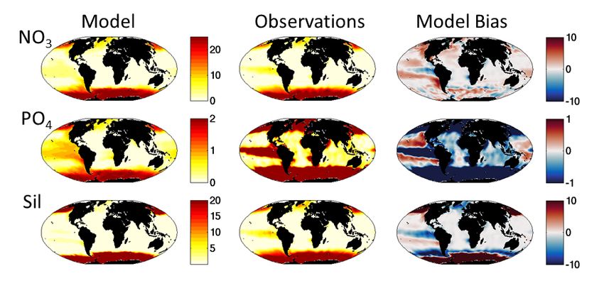
S1.4. Model Parameters: We provide the values for the non-allometric parameters mentioned in the text
above in Supplemental Table 1 and for the allometric parameters in Supplemental Table 2. We refer the
reader to Dutkiewicz et al (2015a) Tables 1 and 2 for the values of all other ecological and biogeochemical
parameters used in this model. We note here only the few changes in parameter values: In Dutkiewicz et
al (2015a) we had preferential remineralization of dissolved organic phosphorus (DOP) relative to other
elements, here we do not. In this study, DOP remineralizes with same values (0.0333 d-1) as the other
elements. We found that CDOM was too high in this version of the model and increased the CDOM
bleaching rate to 0.2592 d-1 from 0.167 d-1.

S2. Model Evaluation

We evaluate the model against a range of in situ and satellite-derived observations (Main text Figs 1,5,7,
and Supplemental Figs S3-S8). The model captures the patterns of low and high surface nutrients seen in
the compilation of in situ observation from World Ocean Atlas (Garcia et al., 2014, Supplemental Fig S3).
Nitrate is slightly too high in the Pacific gyres and too low along the equator. This reflects that iron
limitation may be too strong in this region. But the correlation to observations is good (Supplemental Fig
S5). Phosphate has similar, but accentuated, biases in the Pacific Equatorial region, and is also too high in
the Southern Ocean. Phosphate is thus more evenly distributed than observed (Supplemental Fig S5).
Likely the fixed stoichiometry of the model leads to phosphate concentrations not being sufficiently
biologically modulated. Silicic acid also shows similar biases in the Equatorial Pacific and is too high in the
Southern Ocean. This latter bias is likely a reflection of constant Si:C we impose. In the Southern Ocean,
diatoms are often more highly silicified than in many other parts of the ocean (Tréguer et al 2017). This
overestimation in the Southern Ocean leads to a higher spatial standard deviation relative to the
observations (Supplemental Fig S5).

Chl-a compares well to satellite estimate (Supplemental Fig S4, S5). Note that the satellite estimates have
large uncertainties (Moore et al, 2009 estimates more the 35% errors) and, moreover, the values shown
for the satellite Chl-a estimates in Supplemental Fig S4 are not true annual means, but rather compilations
of all available data, missing values when there are clouds or the light levels are too low (e.g. polar
winters). The coarse resolution of the model does not capture important physical processes near
coastlines, and lack of sedimentary and terrestrial supplies of nutrients and organic matter lead to Chl-a
being too low in these regions. Chl-a is under-estimated by the model in the subtropical gyres, likely due
to lack of mesoscale processes in the model that would supply additional nutrients in these regions (see
e.g. Clayton et al 2017). The model Chl-a is higher than the satellite estimates in the high latitudes.
Regional biases in the satellite algorithms are likely, particularly an issue in the Southern Ocean (e.g. Szeto
et al., 2011, Johnson et al. 2013). The model though has a good correlation with the observations and
captures the spatial variability well (Supplemental Fig S5).

We further compare the model to satellite-based estimates of Chl-a in different size classes (Main Text
Fig 7, Supplemental Fig S4, S5), using the product from Ward et al (2015). Here we capture the ubiquitous
pico-phytoplankton and the limitation of the larger size classes to the more productive regions. The model
pico-phytoplankton size class Chl-a is potentially slightly too low and the nano size class too high. Though
we note that if we set the pico/nano break at the model 5th size class (just under 3µm) instead at the 4th

4

(2µm) size class, the relative values are much more in line with the satellite product. We suggest that the
satellite product division might not be that exact. The micro-size class matches in location to the satellite
product but is slightly too low as discussed above, but has the least impressive correlation to the
observations (Supplemental Fig S5).

We also compare the model functional group distribution to the compilation of observations (Main Text
Fig 7b, MAREDAT, Buitenhuis et al 2013, and references therein). The observations are sparse and here
we average all observations regardless of season in 5 degree bins. With such spatially and temporally
sparse observations, we do not believe it makes sense to calculate biases or correlations between the
model and observations, and we rely on visual evaluation. Though the observations are sparse, we do
capture the ubiquitous nature of the pico-phytoplankton, the limited domain of the diazotrophs (including
observed lack of diazotrophs in the South Pacific gyre), the pattern of enhance diatom biomass in high
latitude, and low in subtropical gyres. We over-estimate the coccolithophore biomass relative to
MAREDAT in many regions, but note that the conversion from cells to biomass in that compilation was
estimated to have uncertainties of several 100% (O’Brien et al., 2013). The MAREDAT compilation did not
include a category for dinoflagellates.

We further evaluate the model against the in situ observations as captured during the Atlantic Meridional
Transects (AMT) 1,2,3, and 4 (Main Text Fig 1, 5, Supplemental Figs S6,S7,S8). AMT2 and 4 occurred during
April and May of consecutive years, while 1 and 3 took place during September and October. Here we
compare the range of values found in the two cruises in each time period to the range of values in the
model during the two-month period (Supplemental Figs S6,S7). Similar to the global evaluation above, we
find that silicic acid is too high in the Southern Ocean (Supplemental Fig S6) and that Chl-a is
underestimated in the subtropical gyres. We note that the model Chl-a compares better to the Southern
Ocean in situ observations than they do to the satellite estimates. Though the correlation is reasonable,
the spatial variability is too low (Supplemental Fig S8a,b). The phytoplankton functional groups compare
less well to observations than the nutrients and Chl-a, but are still plausible. Coccolithophore biomass
however drops too low in the Southern Ocean, likely due to the model smallest diatom being
parameterized as too competitively advantaged. However, pleasingly, the relative abundances of the
three groups (diatoms, coccolithophores and dinoflagellates) are captured: Diatom biomass is much lower
in the subtropical gyres than the other two functional groups, and higher in the Southern Ocean and
coccolithophores and dinoflagellates as having much more even distributions. Note also that
coccolithophore biomass from model compares much better to the AMT data than the MAREDAT
compilation.

As a final model evaluation, we compare the model estimates of richness against those found along the
AMT (Main Text Fig 1, Supplemental Fig S7, S8b,c). As expected, given the only 350 species parameterized
in the model, the model has lower diversity than seen in the AMT. But, the model does captures the low
and high patterns of total richness along the AMT (Supplemental Fig S7a,d), though underestimates the
diversity in the subtropical gyres. In these regions it is likely that traits axes (e.g. symbiosis, colony
formation etc) not captured in the model provide additional means for phytoplankton to co-exist. The
richness within different functional groups is also captured, though much better for diatoms than the
other two groups (Supplemental Figs S7b,e, S8c,d). Excitingly the model also captures the differences in
the diversity within functional groups and in size classes. Diatoms have much larger diversity in the
Southern Ocean than the other functional groups, while coccolithophores and mixotrophic dinoflagellates
diversity is much more uniform across the transect. AMT richness was also calculated for different size

5

classes. The model does well in capturing these divisions (Supplemental Fig S7c,f, S8c,d). The model
captures the much higher diversity within the smallest size category (2-10µm) and the lower and much
more regionally varying diversity in the larger size category, including the lack of diversity in the largest
size class (>20µm) in the subtropical gyres.

S3. Shannon Index

Though richness is a more applicable measure of diversity for this study, where our theory determines co-
existence, here we also provide the Shannon Index (H). Shannon diversity is determined as:
 
 = − ∑ ln Eq. S3.1
 
Where Bj is the biomass of the j-th phytoplankton class, group, or norm (depending on whether
considering total, size, functional, or thermal Shannon index), and biomass of all the phytoplankton is BTOT.
Shannon diversity therefore also includes a measure of how evenly the biomass is distributed. A higher
Shannon index suggests a more evenly distributed community. We show these here normalized to the
maximum value for each dimension (or total), that is if the biomass was evenly distributed between all
types/classes/groups/norms (depending on which dimension). We find that size classes have the highest
Shannon over most of the globe, while the temperature norms have the lowest Shannon (Supplemental
Fig S13).

6

Supplemental References
Baird, M.E., One, R.R., Suthers, I.M., & Middleton, J.H. 2004. A plankton population model with
 biomechanics descriptions of biological processes in an idealized 2D ocean basin. J. Mar, Sys. 50,
 199-222 (2004)

Bec, B., Collos, Y., Vaquer, A. et al. Growth rate peaks at intermediate cell size in marine photosynthetic
 picoeukaryotes. Limnol. Oceanogr., 53, 863–867 (2008)

Bissenger, J.E., Montagnes, D.J.S., Harples, J., & Atkinson, D. Predicting marine phytoplankton maximum
 growth rates from temperature: Improving on the Eppley curve using quantile regression, Limnol.
 Oceangr., 53, 487-493 (2008)

Boyd et al. Marine phytoplankton temperature verus growth response from polar to tropical waters –
 outcome of a scientific community-wide study. PlosOne, 8(5), e63091 (2013)

Buitenhuis, E.T. Vogt, M., Moriarty, R., Bednaršek, N., Doney, S.C., Leblanc, K., Le Quéré, C., Luo, Y.-W.,
 O'Brien, C., O'Brien, T., Peloquin, J., Schiebel, R. and Swan, C.: MAREDAT: towards a world atlas of
 MARine Ecosystem DATa Earth Syst. Sci. Data, 5, 227-239, 2013.

Clayton, S. Dutkiewicz, O. Jahn, C.N. Hill, P. Heimbach, and M.J. Follows. Biogeochemical versus
 ecological consequences of modeled ocean physics. Biogeosciences, 14, 2877-2889 (2017).

Dutkiewicz, S., Hickman, A.E., Jahn, O., Gregg, W.W., Mouw, C.B. & Follows, M.J. Capturing optically
 important constituents and properties in a marine biogeochemical and ecosystem
 model. Biogeoscience, 12, 4447-4481 doi:10.5194/bg-12-4447-2015 (2015a)

Dutkiewicz, S., Morris, J., Follows, M.J., Scott, J., Levitan, O., Dyhrman, S. & Berman-Frank, I. Impact of
 ocean acidification on the structure of future phytoplankton communities Nature Climate Change,
 doi:10.1038/nclimate2722 (2015b)

Eppley, R. W. Temperature and phytoplankton growth in the sea, Fish. B., 70, 1063–1085 (1972)

Fenchel, T. Ecology—Potentials and Limitations. Excellence in Ecology: Book 1. Otto Kinne (ed). Ecology
 Institute. 187 pp. (1987)

Finkel, Z. and AJ Irwin (2000) Modeling size-dependent photosynthesis: light absorption and the
 allometric rule. J. theor. Biol. 204: 361-369. 10.1006/jtbi.2000.2020

Finkel, Z. V., J. Beardall, J., Flynn, K.J., Quigg, A., Rees, T.A.V., & Raven, J.A.. Phytoplankton in a changing
 world: cell size and elemental stoichiometry. J. Plankton Res. 32, 119–137 (2010)

Follows, M.J, Dutkiewicz, S., Ward, B.A., and Follett, C.N. Theoretical interpretation of subtropical
 plankton biogeography. In Microbial Ecology of the Oceans, 3rd Edition, Editors, J. Gasol, D Kirshman.
 Hoboken, NJ, John Wiley, p. 467, 2018.

Garcia, H. E., R. A. Locarnini, T. P. Boyer, J. I. Antonov, O.K. Baranova, M.M. Zweng, J.R. Reagan, D.R.
 Johnson, 2014. World Ocean Atlas 2013, Volume 4: Dissolved Inorganic Nutrients (phosphate,
 nitrate, silicate). S. Levitus, Ed., A. Mishonov Technical Ed.; NOAA Atlas NESDIS 76, 25 pp.

7

Geider, R. J., MacIntyre, H. L., & Kana, T. M. A dynamic regulatory model of photoacclimation to light,
 nutrient and temperature, Limnol. Oceanogr., 43, 679–694 (1998)

Gregg, W. W.A Coupled Ocean–Atmosphere Radiative Model for Global Ocean Biogeochemical Model,
 NASA Technical Report Series on Global Modeling and Data Assimilation, NASA/TM-2002-104606,
 22, NASA, Goddard Space Flight Center, Greenbelt, MD (2002)

Hansen, B.B., Bjornsen, B.W., & Hansen, P.J. Zooplankton grazing and growth: Scaling within the 2– 2000
 mm body size range. Limnol. Oceanogr. 42, 687–704, doi:10.4319/lo.1997.42.4.0687 (1997)

Holling, C. S. Some characteristics of simple types of predation and parasitism, Canadian Entomologist,
 91(7), 385-398 (1959)

Jeong, H.J., Yoo Y.D., Kim, J.S., Seon K.A., Kang, N.S., & Kim, T.H. Growth, Feeding and Ecological Roles of
 the Mixotrophic and Heterotrophic Dinoflagellates in Marine Planktonic Food Webs. Ocean Sci. J.
 45(2):65-91, doi: 10.1007/s12601-010-0007-2 (2010)

Johnson, R., Strutton, P.G., Wright, S.W., McMinn, A., and Meiners, K.M.: Three improved Satellite
 Chlorophyll algorithms for the Southern Ocean, J. Geophys. Res. Oceans, 118,
 doi:10.1002/jgrc.20270, 2013

Kempes, C.P., Dutkiewicz, S. &Follows, M.J. Growth, metabolic partitioning, and the size of
 microorganisms. Proceedings of the National Academy of Science, 109, 495-500,
 doi:10.1073/pnas.1115585109 (2012)

Kiorboe, T. A mechanistic approach to plankton ecology. Princeton University Press. 224 pp (2008)

Maranon E, Cermeno P, Lopez-Sandoval DC, Rodrıguez-Ramos T, Sobrino C, et al. Unimodal size scaling
 of phytoplankton growth and the size dependence of nutrient uptake and use. Ecol Lett 16: 371–379
 (2013)

Monteiro, F.M., Bach, L.T., Brownlee, C., Brown, P., Rickaby, R.E.M., Tyrrell, T., Beaufort, L., Dutkiewicz,
 S., Gibbs, S., Gutowska, M.A., Lee, R., Poulton, A.J., Riebesell, U., Young, J., Ridgwell, A. Why marine
 phytoplankton calcify? Science Advances, 2, doi: 0.1126/sciadv.1501822 (2016).

Montagnes, D.J.S., Berges, J.A., Harrison, P.J., and Taylir, F.J.R. Estimating carbon, nitrogen, protein and
 chlorophyll a from volume in marine phytoplankton. Limnol. Oceanogr., 39, 1044–1060 (1994).

Moore, T.S., Campbell, J.W., and Dowel, M.D.: A class-based approach to characterizing and mapping
 the uncertainty of the MODIS ocean chlorophyll product. Remote Sensing of Environment, 113,
 2424–2430, 2009.

O’Brien, C. J., Peloquin, J. A., Vogt, M., Heinle, M., Gruber, N., Ajani, P., Andruleit, H., Arístegui, J.,
 Beaufort, L., Estrada, M., Karentz, D., Kopczynska, E., Lee, R., Poulton, A. J., Pritchard, T., and
 Widdicombe, C.: Global marine plankton functional type biomass distributions: coccolithophores,
 Earth Syst. Sci. Data, 5, 259–276, doi:10.5194/essd-5-259-2013, 2013.

8

Pančić, M., Rodriguez Torres, R., Almeda, R., & Kiørboe, T. Silicified cell walls as a defensive trait in
 diatoms. Proceedings of the Royal Society B: Biological Sciences, 286,
 doi.org/10.1098/rspb.2019.0184 (2019)

Raven, J. A.: Why are there no picoplanktonic O2 evolvers with volumes less than 10-19 m3? Journal of
 Plankton Research, 16, 565– 580, 1994.

Sal, S., L. Alonso-Sáez, L., Bueno, J., García, F.C. & López-Urrutia, A. Thermal adaptation, phylogeny, and
 the unimodal size scaling of marine phytoplankton growth. Limnol. Oceanogr., 60, 1212–1221 (2015)

Stramski, D., Bricaud, A., & Morel, A. Modeling the inherent optical properties of the ocean based on the
 detailed composition of the planktonic community, Appl. Optics, 40, 2929–2945 (2001).

Szeto, M., Werdell, P.J., Moore, T.S., and Campbell, J.W. :Are the world’s oceans optically different?, J.
 Geophys. Res., 116, C00H04, doi:10.1029/2011JC007230, 2011.

Taniguchi, D.A.A., M.R. Landry, P.J.S. Franks, & K.E. Selph. Size-specific growth and grazing rates for
 picophytoplankton in coastal and oceanic regions of the eastern Pacific. Marine Ecology Progress
 Series. 509, 87-101 (2014)

Tréguer, P., Bowler, C., B. Moriceau, S. Dutkiewicz, M. Gehlen, K. Leblanc, O. Aumont, L. Bittner, R.
 Dugdale, Z. Finkel, D. Iudicone, O. Jahn, L. Guidi, M. Lasbleiz, M. Levy, and P. Pondaven. Influence of
 diatoms on the ocean biological pump. Nature Geoscience, doi:10.1038/s41561-017-0028-x
 (2017).Thomas, M.K., Kremer C.T., Klausmeier C.A., & Litchman E. A global pattern of thermal
 adaptation in marine phytoplankton. Science, 336, 1085-1088, doi.10.1126/science.1224836 (2012)

Verdy, A., Follows, M.J., & Flierl, G. Evolution of phytoplankton cell size in an allometric model. Marine
 Ecology Progress Series, 379, 1-12 (2009)

Ward, B.A., Dutkiewicz, S., Jahn, O. & Follows, M.J. A size-structured food-web model for the global
 ocean. Limnol. Oceanogr., 57, 1877-1891 (2012)

Ward B.A.: Temperature-Correlated Changes in Phytoplankton Community Structure Are Restricted to
 Polar Waters. PLOS ONE, 10 (8): e0135581. doi:10.1371/journal.pone.0135581, 2015.

Ward B.A., Marañón E., Sauterey B., Rault J. & Claessen C. The size-dependence of phytoplankton
 growth rates: a trade-off between nutrient uptake and metabolism. The American Naturalist, 189
 (2), 170-177 (2017)

9

Supplemental Tables
 Symbol Value Units
 normalization factor 0.8 Unitless
 for temperature
 function
 -4000 K
 reference temperature 293.15 K
 factor determining BT 3x10-4 1/K
 width of norms
 norm optimum 271.15 to 304.15 in 4K K
 temperature intervals
 decay coefficient for b 4 Unitless
 norms
 palatibility matrix σjk 1 if grazer k is 10 times Unitless
 larger the prey j.
 0.3 if grazer k is 5 or 15
 times larger than prey j
 grazing half saturation 1.5 mmolC/m3
 rate
Supplemental Table S1: Non-allometric ecological parameters mentioned in the Supplemental Text.

 a b Units
 maximum growth rate, pico 0.9 +0.08
 µmax cocco 1.4 -0.08
 diazotroph 0.95 -0.08 1/d
 diatom 3.9 -0.08
 dinoflagellates 1.7 -0.08
 nutrient uptake half NO3 0.17 0.27 mmol N/m3
 saturation constant,
 K
 minimum cell quota N 0.07 -0.17 mmol N/mmol C
 relative to C, Qmin
 maximum nutrient NO3 0.51 -0.27 mmol N/mmol C/d
 uptake rate, Vmax
 sinking phytoplankton 0.28 0.39 m/d
 zooplankton 0.00
 maximum grazing rate, dinoflagellates 10.3 -0.16
 gmax zooplankton30um 30.9 -0.16
Supplemental Table S2: Plankton parameters that scale with size. Parameter=aVb

10

Supplemental Figures.

Supplemental Figure S1: Absorption and scattering spectra. (a) Chl a-specific total absorption by
phytoplankton (m2/mg Chl a); (b) Chl a-specific absorption by photosynthetic pigments (m2/mg Chl); and
(c ) biomass specific scattering by phytoplankton (m2/mgC). Same coloured lines show each size classes
within functional group: red=diatoms; purple=mixotrophic dinoflagellates; dark blue=coccolithophores;
light blue=diazotrophs; green=pico-phytoplankton; black=zooplankton (only scattering).

11

Supplemental Figure S2: Maximum grazing rate as a function of size. Small symbols indicate results from
laboratory experiments, compiled by Taniguchi et al. (2014), Jeong et al. (2010) and Hansen et al. (1997).
Values were Q10 temperature corrected to 20oC using value of 2.8 (Hansen et al., 1997). Purple diamonds
indicate mixotrophic dinoflagellates, black square for heterotrophic dinoflagellates, black circles for other
protistan grazers, black crosses for metazoan grazers. Note that these metazoans from Hansen et al (1997)
are mostly coastal species and many have non-planktonic life stages; the open ocean groups that the
model is attempting to capture are therefore not represented properly here. The large black circles
indicate the parameter values for the 16 model zooplankton size classes (the model does not differentiate
between functional groups of heterotrophic zooplankton). The large purple diamonds indicate the values
used for the model mixotrophic dinoflagellates.

12

Supplemental Figure S3: Annual Mean Surface (0-10m) Nutrients. (Top row) Nitrate (mmolN/m3);
(Middle row) Phosphate (mmolP/m3); (Bottom row) Silicic acid (mmolSi/m3). (Left column) Model, 5th
year annual mean; (Middle column) Observations, annual climatology, from World Ocean Atlas (Garcia et
al 2013); (Right Column) Model bias determined as model minus observation.

13

Supplemental Figure S4: Annual Mean Surface Chl-a (mgChl/m3). (Top row) total Chl-a; (Second row)
Chl-a in micro (>20μm) size class; (Third row) Chl in nano (2-20μm) size class; (Bottom row) Chl in pico
(

Supplemental Figure S5: Taylor Diagram of Global Annual Surface Fields. This polar coordinate plot
shows correlation (angular position) and the normalized (by observed spatial STD) spatial standard
deviation (radial position) between model and observation for the fields shown in Supplemental Figures
S3 and S4. Statistics are performed on log-normalized fields. REF indicates a perfect match between model
and observations. NO3, PO4, SIL refer to nitrate, phosphate and silicic acid respectively; Observations are
from World Ocean Atlas (Garcia et al 2014). CHL refers to total Chl-a; Observations are satellite estimates
from NASA MODIS. Mic, Nan, Pic refer to Chl-a in the micro (>20μm), nano (2-20μm), pico (

Supplemental Figure S6: Atlantic Meridional Transect Model and In situ Observations. (Left Column)
April/May (AMT2,4); (Right Column) September/October (AMT1,3). Circles indicates average of the two
AMT cruises in 4o latitude bins in each time period, and the vertical line across each circle shows the range
of the observations. Solid curves indicate the model two-month mean and dashed lines indicate the model
minimum and maximum from that two-month period. (a), (b) surface nutrients (black=nitrate,
mmolN/m3; green=phosphate, x16 mmolP/m3; light blue=silicic acid, mmolSi/m3); (c), (d) surface Chl-a
(mg Chl/m3); (e), (f) surface phytoplankton biomass (mg C/m3) (red=diatoms; blue=coccolithophores;
purple=dinoflagellates).

16

Supplemental Figure S7: Atlantic Meridional Transect Model and In situ Observations of richness. (Left
Column) April/May (AMT2,4); (Right Column) September/October (AMT1,3). Circle indicates average of
the two AMT cruises in each time period in 4o latitude bins, and the vertical line across each circle shows
the range of the observations. Solid curves indicate the model two-month mean and dashed lines indicate
the model minimum and maximum from that two-month period. Normalized richness of (a),(d) all
diatoms, coccolithophores and dinoflagellates together; (b),(e) each functional groups separately (red:
diatoms, dark blue: coccolithophores, purple: dinoflagellates); (c),(f) 3 size classes (light blue: 2-10µm,
black: 10-20µm, green: >20µm). Model pico-phytoplankton and diazotrophs are not included in the model
analysis as they were not analyzed in the observations.

17

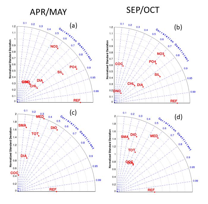
Supplemental Figure S8: Taylor Diagram of Atlantic Meridional Transect Fields. This polar coordinate
plot shows correlation (angular position) and the normalized (by observed spatial STD) spatial standard
deviation (radial position) between model and observation for the fields shown in Supplemental Figures
S6 and S7. (Left Column) April/May (AMT2,4); (Right Column) September/October (AMT1,3). We compare
the in situ two-cruise mean (circles in Supplemental Fig S6 and S7) against the model two-month average
(solid lines) averaged onto the same 4o latitude bins. REF indicates a perfect match between model and
observations. (a),(b) NO3, PO4, SIL refer to nitrate, phosphate and silicic acid respectively. CHL refers to
Chl-a. DIA, COC, DIO refer to diatom, coccolithophore and dinoflagellate biomass respectively. Statistics
are performed on log-normalized fields for the Chl-a and biomass fields. (c),(d) normalized richness where
TOT refers to the total richness DIA, COC, DINO refers to the richness in diatoms, coccolithophores, and
dinoflagellates respectively, and SMA, MED, LAR to the 3 size classes (2-10µm, 10-20µm, >20µm)
respectively.

18

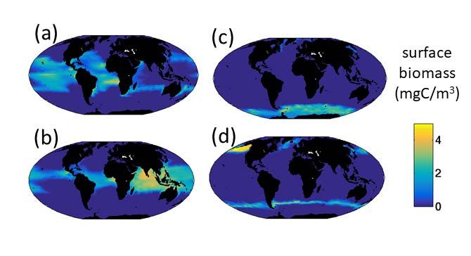
Supplemental Figure S9: Representative phytoplankton type distributions. Surface annual mean
biomass (mgC/m3) of four of of the 350 types distributions. (a) and (b) are warm adapted small
prokaryotes, (c) and (d) are cold adapted small diatoms. These are the types indicated with A,B,C,D in
Main Text Fig 6.

19

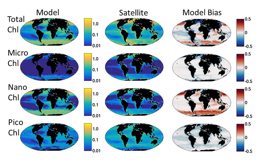
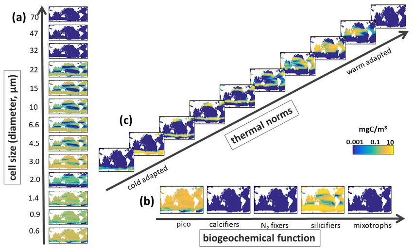
Supplemental Figure S10. Default Model Biomass along Different Trait Axes. Annual mean carbon
biomass (mg C/m3) over top 100m of (a) Sizes classes with equivalent spherical diameters (ESD) as labelled
on Y-axis, shown is the sum across all functional groups and all temperature norms in that size classes; (b)
Biogeochemical functional groups (pico-phytoplankton, coccolithophores, diazotrophs, diatoms and
mixotrophic dinoflagellates) summed across all size classes and all temperature norms in those groups;
and (c) thermal norms from coldest adapted to warm adapted (see Main Text Fig 3), summed across all
functional groups and size class.

20

Supplemental Figure S11. Default model zooplankton biomass (mgC/m3). Arranged by size (given as
equivalent spherical diameter, ESD, on Y axis).

21

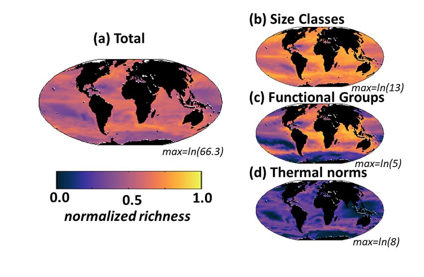
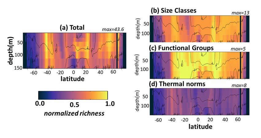
Supplemental Figure S12. Default model diversity measured as annual mean normalized richness with
depth along a transect at 30W in the Atlantic Ocean. Normalization is the maximum in the transect for
the total or the particular dimension (noted above each panel). (a) total richness determined by number
of individual phytoplankton types (of the 350) that co-exist at any location; (b) size class richness
determined by number of co-existing size classes; (c) functional richness determined by number of co-
existing biogeochemical functional groups; (d) thermal richness determined by number of co-existing
temperature norms. Total richness (a) is a multiplicative function of the three sub-richness categories (b-
d). Contours indicate total phytoplankton carbon biomass. Black indicates land/islands.

22

Supplemental Figure S13. Default model normalized annual mean Shannon diversity at the surface. (a)
total Shannon; (b) size class Shannon determined from co-existing size classes; (c) functional Shannon
determined from co-existing biogeochemical functional groups; (d) thermal Shannon determined from
co-existing temperature norms. All panels are normalized to the maximum value for that dimension (or
total) as natural log of the maximum number of potentially coexisting types/classes/groups/norms (values
noted below each panel).

23

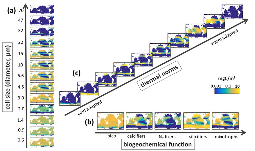
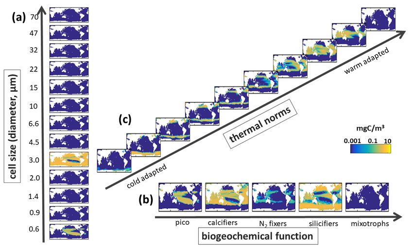
Supplemental Figure S14. EXP-1 Model Biomass along Different Trait Axes. Sensitivity experiment where
there is no mixotrophy and only a single grazer type preys on all phytoplankton. Annual mean carbon
biomass (mg C/m3) over top 100m of (a) Sizes classes with equivalent spherical diameters (ESD) as labelled
on Y-axis, shown is the sum across all functional groups and all temperature norms in that size classes; (b)
Biogeochemical functional groups (pico-phytoplankton, coccolithophores, diazotrophs, diatoms and
dinoflagellates) summed across all size classes and all temperature norms in those groups; and (c) thermal
norms from coldest adapted to warm adapted (see Main Text Fig 3), summed across all functional groups
and size classes. Compare to Supplemental Fig S10.

24

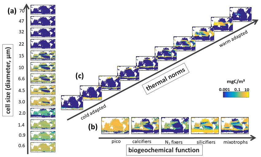
Supplemental Figure S15. EXP-2 Model Biomass along Different Trait Axes. Sensitivity experiment where
nutrient requirements are the same between functional group. Annual mean carbon biomass (mg C/m3)
over top 100m of (a) Sizes classes with equivalent spherical diameters (ESD) as labelled on Y-axis, shown
is the sum across all functional groups and all temperature norms in that size classes; (b) Biogeochemical
functional groups (pico-phytoplankton, coccolithophores, diazotrophs, diatoms and dinoflagellates)
summed across all size classes and all temperature norms in those groups; and (c) thermal norms from
coldest adapted to warm adapted (see Main Text Fig 3), summed across all functional groups and size
classes. Compare to Supplemental Fig S10.

25

Supplemental Figure S16. EXP-3 Model Biomass along Different Trait Axes. Sensitivity experiment where
there is no horizontal transport of plankton, however nutrients and dissolved and detrital organic matter
are transported as in the default experiment. Annual mean carbon biomass (mg C/m3) over top 100m of
(a) Sizes classes with equivalent spherical diameters (ESD) as labelled on Y-axis, shown is the sum across
all functional groups and all temperature norms in that size classes; (b) Biogeochemical functional groups
(pico-phytoplankton, coccolithophores, diazotrophs, diatoms and dinoflagellates) summed across all size
classes and all temperature norms in those groups; and (c) thermal norms from coldest adapted to warm
adapted (see Main Text Fig 3), summed across all functional groups and size classes. Compare to
Supplemental Fig S10.

26