Autonomous Head-to-Head Racing in the Indy Autonomous Challenge Simulation Race
←
→
Page content transcription
If your browser does not render page correctly, please read the page content below
Autonomous Head-to-Head Racing in the Indy Autonomous Challenge
                                                                 Simulation Race
                                                                             Gabriel Hartmann1,2 , Zvi Shiller1 , and Amos Azaria2

                                            Abstract— This paper describes Ariel Team’s autonomous                   and is based on a race car of the Indy Lights series. The
                                         racing controller for the Indy Autonomous Challenge (IAC)                   official simulator for the IAC is the Ansys VRXPERIENCE
                                         simulation race [1]. IAC is the first multi-vehicle autonomous              simulator [2], which simulates the AV-21 dynamics and
                                         head-to-head competition, reaching speeds of 300 km/h along
                                         an oval track, modeled after the Indianapolis Motor Speedway                the IMS track (see Fig. 2). Prior to the competition, all
                                                                                                                     teams were required to demonstrate autonomous control of
arXiv:2109.05455v1 [cs.RO] 12 Sep 2021

                                         (IMS).
                                            Our racing controller attempts to maximize progress along                a real vehicle (see [3] for the demonstration submitted by
                                         the track while avoiding collisions with opponent vehicles and              our team). During the development period, which lasted 16
                                         obeying the race rules. To this end, the racing controller first            months, there were three testing events that gradually led to
                                         computes a race line offline. Then, it repeatedly computes online
                                         a small set of dynamically feasible maneuver candidates, each               the final simulation race. The simulation race is composed
                                         tested for collision with the opponent vehicles. Finally, it selects        of four parts: solo laps, in which all vehicles drive alone;
                                         the maneuver that maximizes progress along the track, taking                safety tests that validate the ability of each vehicle to avoid
                                         into account the race line.                                                 collisions and obey the race rules; semi-finals, in which the
                                            The maneuver candidates, as well as the predicted trajecto-              place in the grid is set according to the solo lap times; and
                                         ries of the opponent vehicles, are approximated using a point
                                         mass model. Despite the simplicity of this racing controller, it            the final race.
                                         managed to drive competitively and with no collision with any
                                         of the opponent vehicles in the IAC final simulation race.

                                                                 I. I NTRODUCTION
                                            The Indy Autonomous Challenge (IAC) is an international
                                         competition, organized by Energy System Network (ESN),
                                         intended to promote the development of algorithms driv-                     Fig. 2: The VRXPERIENCE simulator used for the simula-
                                         ing under challenging conditions. The IAC of 2020-2021                      tion race.
                                         is the world first multi-vehicle, high speed, head-to-head
                                         autonomous race held on the Indianapolis Motor Speedway
                                         (IMS). Over 30 teams from universities around the globe
                                                                                                                     A. Challenges of autonomous racing
                                         participated in the challenge. The competition is carried out
                                                                                                                        Autonomous racing has unique challenges, emanating
                                                                                                                     from the unique properties of the race vehicle, its extreme
                                                                                                                     speeds, and the competitive nature of the driving.
                                                                                                                           a) Extreme speeds: Racing speeds coupled with limited
                                                                                                                     frequencies of the sensor readings lead to state updates at
                                                                                                                     large distance intervals compared to the vehicle size and the
                                                                                                                     distance between neighboring vehicles. Furthermore, driving
                                                           (a)                                  (b)                  near the vehicle’s performance envelope at close proximity
                                                                                                                     to neighboring vehicles leaves little room for correction and
                                         Fig. 1: (a) The Indianapolis Motor Speedway (b) the AV-12
                                                                                                                     hence requires high fidelity prediction of the behavior of the
                                         autonomous race car.
                                                                                                                     opponent vehicles.
                                                                                                                           b) Competitive driving: Competitive driving forces the
                                         in two stages: a simulation race, and a real race on IMS with
                                                                                                                     competitors to race at close proximity to opponent vehicles
                                         the Dallara AV-21, which reaches speeds of up to 300 km/h
                                                                                                                     and to often block other vehicles from passing. As a result,
                                           This research was supported, in part, by the Ministry of Science &        the time difference between the leading teams is in the order
                                         Technology, Israel.                                                         of a fraction of a second. This in turn forces all competitors
                                           This work has been submitted to the IEEE for possible publication.        to drive on the performance envelop of the vehicle and the
                                         Copyright may be transferred without notice, after which this version may
                                         no longer be accessible.                                                    driver, leaving little room for safety. Although the goal is to
                                           1 Department of Mechanical Engineering and Mechatronics, Ariel Uni-
                                                                                                                     win the race, in our opinion, especially at the first time that
                                         versity, Israel                                                             such head-to-head race is taking place, safer behavior and
                                           2 Department of Computer Science, Ariel University, Israel
                                           gabrielh@ariel.ac.il, shiller@ariel.ac.il,                                larger safety margins should be preferred over pushing the
                                         amos.azaria@ariel.ac.il                                                     performance to the limits.
c) Aerodynamics forces: The aerodynamics of a race RRT* (Rapid Random Tree) search [19].
car has two main effects: a down-force that increases the Trajectory tracking can be accomplished using simple
tire grip and lets the car reach a lateral acceleration of geometric controllers or more complex controllers that takes
over 2.5g, which allows driving at maximal speeds along the vehicle dynamics directly into account [20].
an oval track. The second effect is a slipstream, or draft,
which reduces the drag on the following vehicle. This allows C. This paper
vehicles of identical dynamics to overtake each other. The The autonomous racing controller, developed by “Ariel
racing rules [4] are derived from the rules used in human- Team”, was developed under the underlying principle, which
driven races. An important principle is that an overtaking must guide all developers of autonomous vehicles, that em-
vehicle is responsible to avoid collision with a vehicle that phasizes safety over performance. To this end, our controller
is moving on its race line, while the overtaken vehicle is attempted to avoid collisions, even if the race rules placed the
expected to maintain its own race line. In the simulated race, responsibility to avoid the collision on the opponent vehicle.
a vehicle is disqualified if it leaves the track. The racing controller is based on a repeated search for the
locally best maneuver that avoids collisions with opponent
B. Related Work vehicles, attempts to follow the globally optimal race line,
Unlike the IAC which is a head-to-head autonomous race, and obeys the race rules.
other autonomous racing competitions of full-size vehicles, A set of local maneuvers are generated at 25Hz, using a
traveling at high speeds, such as the formula student chal- point mass model from the current state to a small set of
lenge [5] or Roborace [6], focus mainly on solo racing. discrete points along the track. At each step, the selected
In solo racing, since it is not required to attend to other maneuver is tracked using pure-pursuit and a proportional
vehicles, one must drive the vehicle along a time-optimal velocity controller. Our approach resembles the approach
race line at time-optimal speeds. This was achieved using used in [21], [22] for urban driving.
model predictive control (MPC) [7], [8] and reinforcement It is interesting to note that despite its simplicity, our
learning [9], [10]. controller demonstrated competitive driving while overtaking
Racing against multiple vehicles is more challenging than other vehicles, staying within a close range of the leading
solo racing as it requires the online prediction of the tra- vehicle, and not being involved in any collision throughout
jectories of the neighboring vehicles, and the planning of the race. Furthermore, our vehicle maintained the 3rd place
a dynamically safe avoidance maneuver. A survey of early for a major part of the semi-finals and the finals. We ended
prediction methods is presented in [11]. An early approach to up getting off the track, with 3 laps to go, while avoiding a
trajectory prediction uses Kalman filter assuming a constant vehicle that entered our safety bound. This placed us 6th in
velocity and acceleration [12]. A more recent approach uses the final simulation race.
recurrent neural networks to predict multi modal distribution
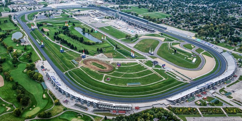
of future trajectories [13]. II. S OFTWARE A RCHITECTURE
Two main approaches for driving in dynamic environments
have emerged: one generates online control commands, Simulator Online Offline
whereas the other tracks a selected trajectory. Cameras
Perception
Online control commands can be generated using MPC to
Radar Prediction
repeatedly optimize a forward trajectory, while accounting Map
for geometric constraints, moving opponent vehicles, and Ego-vehicle
State Estimation
state
ego-vehicle dynamics. MPC was demonstrated in [8] to
avoid static obstacles, and in [14] to drive competitively in Optimal
Trajectory planner
a head-to-head race with two vehicles. Another method to race line
online generate control commands is based on the concept Control
Velocity control Trajectory following
commands
of Velocity Obstacles (VO), which maps static and dynamic
obstacles (e.g. opponent vehicles) to the velocity space of
the ego vehicle [15], [16]. This allows an efficient selection Fig. 3: Software Architecture.
of a collision free velocity that avoids an arbitrary number
of vehicles. The software architecture is shown schematically in Fig
The second approach for driving in dynamic environments 3. For a given track map, we first compute an optimal
divides the driving task into two simpler sub-tasks: first race line, offline, which will serve us throughout the race.
plan a trajectory, then track this trajectory using a tracking The data from the cameras and radars provide the position
controller. The trajectory planner can be simplified by using a and velocity of the surrounding opponent vehicles, and
simple dynamic model to compute a collision free trajectory. additional simulated sensors provide the ego-vehicle state
The tracking controller then tracks the trajectory without e.g., position and velocity. These data, together with the map
considering the obstacles. and the optimal race line, are used by the prediction module
The trajectory can be computed using a graph search in a to repeatedly predict future trajectories of the opponent
spatiotemporal lattice [17], in a spatial lattice [18], or by an vehicles. The same information is used by the trajectory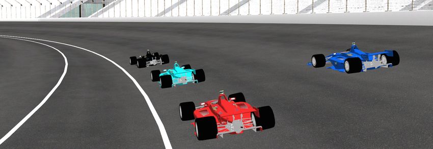
planner to plan an optimal local maneuver for the ego-
vehicle. This maneuver serves as an input to the trajectory-
following controller, which computes the desired linear and
angular velocities of the ego-vehicle. The linear and angular
velocities are controlled by the velocity controller which
outputs the steering, throttle and brake commands. Fig. 5: Road-aligned coordinate system.
III. C OMPUTING THE OPTIMAL RACE LINE
The optimal race line is a time optimal trajectory computed In our coordinate system for every point (xi , yi ), |xi |
offline, based on the track geometry and vehicle dynamics. represents the distance from the ego-vehicle along the track
The IMS is an oval track, 2.5 miles (4, 023 m) long, as (a negative xi represents a point behind the ego-vehicle), and
depicted in Fig. 4a. yi represents the shift from the boundary regardless of the
We computed the optimal race line using an open-source track shape and the ego-vehicle’s location.
trajectory optimization software, [23]. The optimal race line, B. Computing a trajectory between two point
typically maximizes the radius of curvature by entering the In this section, we explain how two trajectory points
corner on the outside boundary of the track, passing through (a start point and a goal point) are connected to form a
the apex on the inner boundary, to the exit point on the trajectory based on the time-optimal motion of a point-mass
outside boundary, as shown in Fig. 4. model. This method is used for opponent vehicles trajectories
predictions and planning maneuver candidates for the ego-
1400 vehicle.
1200
Let ps = {x0 , y0 , ẋ0 , ẏ0 } be the start point, and let
1000
pg = {xg , yg , ẋg , ẏg } be the goal point. We plan a trajectory
C(t) = {x(t), y(t), ẋ(t), ẏ(t)}, t ∈ [0, T ] that connects
Y[m]
800
the start point with the goal point, i.e, C(0) = ps and
600
C(T ) = pg . For composing the trajectory we first assume
400
that ẋs = ẋg , i.e, the starting velocity (in the x axis) equals
200
the goal velocity, and later re-adjust the velocity. Therefore,
0
0 500 1000
the final time T is:
X[m] xg − x0
T = .
(a) (b) ẋ0
Fig. 4: (a) The IMS track. (b) The optimal race line around C is created by applying a bang-bang lateral force with a
a corner of the track. single switch point on a point mass m, similar to [24].
Let Fy be a force, such that:
√
IV. O NLINE T RAJECTORY P LANNING − 2A − T (ẏg + ẏ0 ) + 2(yg − y0 )
Fy =
The online trajectory planner computes a collision free T 2m
2 2 2
trajectory at 25 Hz with a planning horizon of 200 m. It where, A = (T (ẏ0 + ẏg ) − 2T (yg − y0 )(ẏg + ẏ0 ) +
2
is used as a reference for the trajectory following controller 2(yg − y0 ) ). The bang-bang lateral force is applied in one
(see Section V). The planner first generates 8 dynamically direction until a switching time, Ts , and then the force is
feasible maneuver candidates, then selects the best candidate applied in the opposite direction, i.e., Fy is applied for
that maximizes progress along the path and avoids collision t = [0, Ts ] and −Fy is applied for t = (Ts , T ].
with the opponent vehicles. Since the planning horizon of is m(ẏg − ẏ0 ) + Fy T
limited to 200 m, and the typical driving speed is over 80 m/s, Ts =
2Fy
the time horizon is less than 3 seconds. The small number
of maneuver candidates, generated at 25Hz, and the short Finally, C(t) is computed for t ∈ [0, T ] by:
time horizon, sufficiently span the set of options of possible x(t) = ẋ0 t
feasible maneuvers, as demonstrated in the simulation runs F
presented later in Section VI. ẏt + 21 my t2 t < Ts
y(t) =
A. Coordinate system F
ẏ0 t − 12 my t2 t > Ts
An ego-vehicle- and road-aligned coordinate system is ẋ(t) = ẋ0
used for planning, such that x axis is tangent to the left track F
ẏ0 + my t t < Ts
boundary and the y axis is normal to track. The position of
ẏ(t) =
the ego-vehicle is denoted as (xe , ye ); since the coordinate F
ẏ0 + my (2Ts − t) t > Ts
system is aligned with the ego-vehicle, the ego-vehicle is
always located at xe = 0. ye represents the ego-vehicle’s Fig. 6 illustrates an example of a trajectory that connects
normal shift from the left boundary. (see Fig. 5). two points.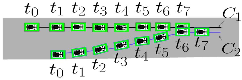
(a)

                               (a)

                                                                                                        (b)
                                                                      Fig. 7: Predicted trajectories of an opponent vehicle (marked
                                                                      as an orange bounding box). Black indicates constant curva-
                                                                                       ˆ and yellow indicates J, which considers
                                                                      ture trajectory J,
               (b)                             (c)                    the track boundaries. In (a) Jˆ exceeds track boundaries;
                                                                      therefore, a lane-changing trajectory is predicted by J; in (b)
Fig. 6: A trajectory between given start and goal points.             although the vehicle drives on a straight line, a lane-keeping
(a) Force Fy is applied on mass m to create a continuous              trajectory is predicted by J.
trajectory between the points. (b) The lateral force Fy profile
and (c) the lateral velocity ẏ(t).
                                                                         We note that our method for trajectory prediction assumes
                                                                      that other vehicles follow a smooth motion profile. The
C. Opponents vehicles’ trajectory prediction                          justification for this assumption relies on the fact that in time
                                                                      horizon, when traveling at high velocity, and since the racing
   An important part of motion planning in a dynamic
                                                                      rules prohibit sudden changes of racing lines, other vehicles
environment and especially in racing is to predict the future
                                                                      are likely to continue their motion profiles.
positions and velocities of all the other vehicles surrounding
the ego-vehicle. Therefore, we develop a prediction module,
                                                                      D. Creating maneuver candidates
which given opponent vehicle state s that contains position
xo , yo , velocity ẋo , ẏo and angular velocity ωo , predicts          The online trajectory planner plans a set of dynamically
the future trajectory J(t) = {x(t), y(t), ẋ(t), ẏ(t)} up to a       feasible maneuver candidates and selects one of them ac-
predefined time horizon Tmax , which we set to 3 seconds.             cording to multiple criteria, as follows.
   Our prediction module first predicts other vehicles future            1) Lane change maneuver: Given ego-vehicle’s state se =
trajectory by assuming that they retain their current steer-          {xe , ye , ẋe , ẏe } and a lateral target ŷ, which defines the target
ing and then updates its prediction according to the track            lane, the planner module creates a lane change maneuver,
boundaries. Namely, for a given opponent vehicle, we first            C ŷ , by connecting the following three trajectory points,
predict a future trajectory, J,   ˆ that keeps a constant curvature   qi = {xqi , yqi , ẋqi , ẏqi }, where i ∈ {0, 1, 2}, as described
κ, which we approximate by: κ = ||ẋoω+oẏo || . However,             in Section 8.
it is expected that the opponent vehicle will consider the               q0 is derived from ego vehicle’s current state se , such that
track boundaries and will avoid exceeding them. Therefore,            q0 = se . The second point defines the lateral distance of the
our prediction module also takes the track boundaries into            desired lane ŷ and the longitudinal lane-changing distance
account and uses the following method. Let (x̂, ŷ) be the            that depends linearly on the lateral changing distance (ŷ −
first position on Jˆ in which the opponent vehicle approaches         ye ) by a predefined factor b and predefined constant c. That
one of the boundaries and is only a distance of dmin from             is, xq1 = {(ŷ − ye )b + c, yq1 = ŷ, ẋq1 = ẋe , ẏq1 = 0}.
it. We define three trajectory points, p0 , p1 and p2 as              The third trajectory point, q2 retains the lane parallel to the
described hereunder, where each trajectory point is composed          boundary up to a maximal longitudinal distance xmax , i.e.,
of pi = {xpi , ypi , ẋpi , ẏpi }; the prediction module connects    xq2 = xmax , yq2 = ŷ, ẋq2 = x˙e , and ẏq2 = 0}. Fig. 8a
them by a point mass maneuver as explained in Section IV-             illustrates a lane change maneuver.
B. The first trajectory point, p0 is derived from the opponent
vehicle’s current state s, such that xp0 = xo ,yp0 = yo ,
ẋp0 = ẋo , and ẏp0 = ẏo . The second trajectory point, p1 ,
is based on (x̂, ŷ), but we assume that the opponent vehicle
will not increase its curvature; therefore, we assume that ŷ
will be reached later on, by a predefined factor, k. That is,
xp1 = (x̂ − xo )k, yp1 = ŷ, ẋp1 = ẋo , ẏp1 = 0}. The third                        (a)                                 (b)
trajectory point, p2 retains the lane parallel to the boundary
up to Tmax , i.e., xp2 = ẋo Tmax , yp2 = ŷ, ẋp2 = ẋo , and        Fig. 8: Illustration of the maneuver candidates planning: (a)
ẏp2 = 0}. Examples of predicted trajectories are shown in            lane change maneuver and (b) a maneuver to the optimal
Fig. 7.                                                               race line.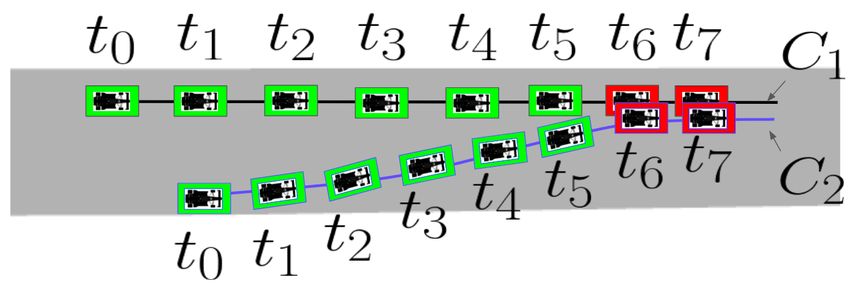
We define N equally spaced lanes, with zero width, which           longitudinal safety bound of 0.6 of a vehicle and a lateral
represent potential ŷ values. The first and last lane are far        safety bound of an entire width of a vehicle. We note that,
enough from the boundaries to allow a vehicle to follow them          while a circular safety bound is more convenient because the
safely. Our planner generates N lane change maneuvers, one            yaw angles of the vehicles are indifferent, since the length
for each defined lane. Let M0 be the set of all lane change           of the race car is more than double its width, a circular
maneuvers. More formally,                                             safety bound would not fit well to the vehicle’s shape. Since
                  −1
                 N[                                                   the slip angles are small, the yaw angles, of the vehicles is
                                              w − 2dmin               approximated by the angle of vehicle’s velocity vector.
         M0 =          C ŷi , ŷi = dmin +             i
                 i=0
                                                N −1                     Two trajectories C1 and C2 describe a collision if there
                                                                      exists some t that the safety bounds of both associated
where dmin is the minimal distance to keep from track
                                                                      vehicles at time t overlap. See Fig. 10 for an illustration.
boundaries. The width of the track in most segments is 14
                                                                         A maneuver candidate is considered free if it does not
m; we set N = 7 to achieve a distance between lanes, that
                                                                      collide with a predicted trajectory of any opponent vehicle.
is close to the vehicles width (2 m).
                                                                      However, if an opponent vehicle is directly behind the ego-
   2) Maneuver to the the optimal race line: In addition
                                                                      vehicle, and the ego-vehicle blocks it, our controller ignores
to these lane-changing maneuvers, we plan a maneuver
                                                                      it, since it is the opponent vehicle’s clear responsibility to
C Jopt , which smoothly merges with the optimal race line
                                                                      avoid a collision.
Jopt . We define the following three trajectory points q̃i =
{xq̃i , yq̃i , ẋq̃i , ẏq̃i }, where i ∈ {0, 1, 2}.
   The first trajectory point q̃0 = se ; the second, q̃1 ∈ Jopt
such that {(yq̃1 −ye )b̃+c̃ = xq̃1 , where b̃ and c̃ are predefined
constants. Finally, q̃2 ∈ Jopt such that xq̃2 = xmax . See Fig.
8b).                                                                                (a)                            (b)
   The full set of the maneuver candidates is M = M0 ∪
  Jopt                                                                Fig. 10: Two trajectories describing the location of each
C       , as shown in Fig. 9.
                                                                      vehicle and its safety bounds. In (a) the vehicles collide at
                                                                      time t6 ; in (b) the vehicles do not collide since the overlap
                                                                      of their safety bounds is at different times.

                                                                      G. Maneuver selection

Fig. 9: Example of 7 lane-changing maneuvers (green) and                 Our planner considers all maneuver candidates that are
a maneuver that merges with the optimal race line (blue).             free. Nevertheless, maneuver candidates that anticipated col-
                                                                      lision with a vehicle when proceeding at maximal velocity,
                                                                      are updated and their velocity is controlled so they do not
E. Velocity re-planning                                               collide, if possible (See Fig. 11).
   Although the maneuver candidates M and the predicted
trajectories of the opponent vehicle include velocities in
addition to positions, these velocities were only used to
define the direction of the paths and to estimate the lateral
forces on the vehicle. Therefore, the velocity profiles are re-
planed to more accurately represent the future motion, by
assuming that the vehicles accelerate along the trajectories
until reaching the maximal velocity. This is possible since our
planned trajectories approximate the vehicle dynamics and             Fig. 11: Updating a maneuver candidate to become free
thus, allow maintaining maximal velocity—without losing               by decelerating toward a blocking vehicle that drives at a
control—when following them.                                          velocity of v2 (green), instead of accelerating to the maximal
                                                                      velocity, vmax (red), and causing a collision.
F. Collision
   To avoid a collision, due to the uncertainly inherent to our          If more than one maneuver is free, each maneuver is
problem, we define a safety bound around the vehicle. We              associated with a cost based on the following criteria; the
attempt not only to avoid a collision with another vehicle but        maneuver with the lowest cost is selected.
also to avoid any overlap between the safety bounds around               1) Maneuver expected time: The time each maneuver is
both vehicles. We use a rectangular safety distance; we define        expected to take until reaching the planning horizon. For
the longitudinal safety bound as 0.3 of the vehicle length            maneuver C, we use T (C) to denote this time. For example,
both front and rear, and the lateral safety distance as 0.5 of        consider two maneuvers, C and C 0 , where C is shorter
the vehicle width, right and left. This results in keeping a          than C 0 , possibly because C 0 contains lane changing. If the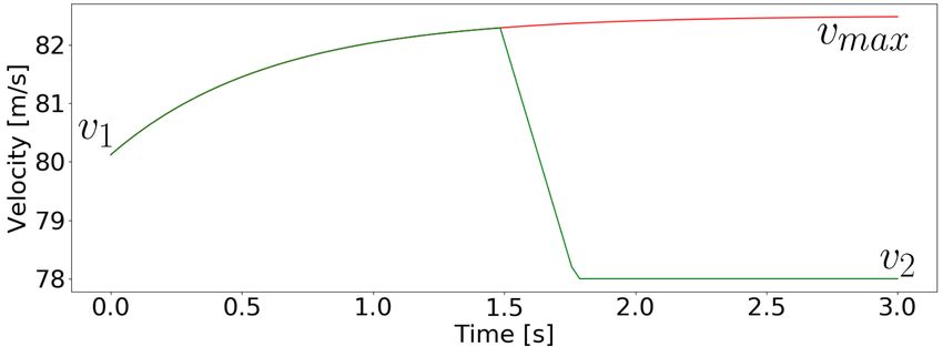
velocity along C and C 0 is equal, then T (C) < T (C 0 ).
However, if C is blocked by another vehicle which requires
decelerating along that path to avoid the collision, it might                                    (a)
be that T (C) > T (C 0 ).
   2) Closest maneuver to the optimal trajectory: The ma-
neuver with the lowest expected time is only locally optimal
                                                                                                 (b)
since the short-horizon maneuver candidates are compared,
but the global optimality is not considered. Incorporating
global optimality into the maneuver candidates would re-
quire predicting and planning to an extended range, which
                                                                                                 (c)
would require extensive computing power and would raise
uncertainty.
   To partially account for global optimality, the planner
prefers maneuvers that come close to the optimal race line,
which is global optimal—without considering other vehicles.                                      (d)
To encourage the selection of a maneuver that is the closest,
among the free candidates, to the optimal race line, that          Fig. 12: Maneuver selection examples, green: free maneu-
maneuver obtains a reward Ro , which controls the trade-           vers, red: blocked maneuvers, blue: chosen maneuver. (a)
off between local time optimality and following the optimal        The planner selects a minimum-time lane-changing maneu-
race line. That is, for a maneuver C, let O(C) be Ro if C is       ver because the current lane is blocked by another vehicle. (b)
closest, among the free candidates, to the optimal race line,      The planner prefers the longer maneuver because it returns to
and 0 otherwise.                                                   the optimal race line (shown in light-blue). (c) The planner
   3) Minimum change from the current trajectory: The              selects a free maneuver that is the closest to the optimal race
selected maneuver can change significantly at every time step      line . (d) None of the maneuver candidates are free, therefore
when the optimality of two maneuver candidates is similar.         the safest maneuver is chosen.
To stabilize the planning, it is preferred, when possible,
to keep the same maneuver, unless another maneuver is
conspicuously better. Clearly, switching to a new maneuver
is more severe if a switch has just occurred, but once some
time has passed since the last switch, the controller should
be more lenient towards another switch.
   For a maneuver C, let K(C) be Rk if C is the same
maneuver as the maneuver that the vehicle currently drives                        Fig. 13: Pure pursuit geometry.
on, and 0 otherwise. Rk drops with a linear decay rate Rd
as long as the maneuver is followed, and is reset to its initial
value Rk0 if the maneuver is switched.                             A. Lateral control
   Finally, the cost associated with each free maneuver C ∈           The pure pursuit algorithm [25] is used to compute the de-
M is T (C) − Oopt(C) − K(C). The maneuver with the                 sired angular velocity based on the current ego-vehicle’s state
minimal cost is selected. Fig. 12 a,b,c show examples of           and the selected maneuver, which is mapped to Cartesian
selected maneuvers.                                                coordinates. The pure pursuit algorithm pursuits a target on
                                                                   the selected maneuver C. Let v be the vector representing the
H. Behavior when no maneuver is free                               ego-vehicle’s velocity. The distance to the target is defined
   Situations in which none of the Maneuvers are free are          to be proportional to the vehicle’s speed v = |v| that is, ld =
unavoidable due to the unpredictable behavior of other             vkt , where kt is a predefined constant. The angle between
vehicles and inaccurately modeled ego-vehicle dynamics. If         the velocity vector v to the vehicle-target vector is denoted
none of the Maneuvers are free, the optimality criteria are        as α (see Fig. 13). The desired angular velocity of the vehicle
not relevant and the only selection criterion is safety. To find   ωd is 2v sin
                                                                             ld
                                                                                α
                                                                                  . The desired angular velocity ωd is used as a
the safest maneuver the planner finds the closest collision        reference for a proportional angular velocity controller that
and selects a maneuver that is as far as possible from that        computes the steering command: δ = (ωd − ω)kω where, ω
collision (see an example at Fig. 12d).                            is the current angular velocity of the vehicle, and kω is a
                                                                   proportional gain.
                        V. C ONTROL                                B. Longitudinal control
   The control module outputs throttle, brake, and steering          The desired speed vd is provided by the selected maneuver,
commands that drive the vehicle as close as possible to the        which is usually used as a reference for the longitudinal
selected maneuver.                                                 controller. However, when closely following a vehicle, we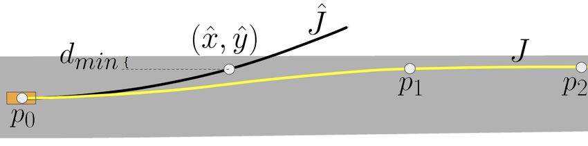
modify the desired speed to be: vd = vf −(Ld −L)kf , where        this phenomenon happened during our testing, despite all
vf is the speed of the leading vehicle, L is the distance to      vehicles using the same controller. Fig. 16 demonstrates an
the leading vehicle, Ld is the desired distance to keep, and      overtake maneuver with 3 vehicles, all using our controller.
kf is a proportional gain. This modification allows smooth        At every corner, the black vehicle gains a small advantage
driving and keeping a constant distance from the leading          over the blue vehicle until it successfully completes the
vehicle. Fig. 14 illustrates a following scenario. Finally, the   overtaking maneuver.

Fig. 14: Following a vehicle. The distance between the ego-
vehicle and the vehicle ahead, L, is less than the predefined
following distance, Ld ; therefore, the ego-vehicle will slow
down, to increase L.

throttle and brake command u is computed by a proportional
speed controller: u = (vd − v)kv where, kv is a proportional                           (a)                (b)
gain.                                                             Fig. 15: Snapshots of planning in a crowded scenario with
                     VI. E XPERIMENTS                             5 opponent vehicles.
A. Simulation environment
   The VRXPERIENCE simulator enables multi-vehicle
head-to-head competitions, in which every vehicle is con-
trolled by a separate controller. The sensors are simulated at
25 Hz and the ego-vehicle’s state at 100 Hz, in simulator                        (a)                             (b)
time. Each controller receives the ego-vehicle’s state and
the sensor data from the simulator, and sends back throttle,
brake, and steering commands.
   We used the pre-processed cameras and radars data from                        (c)                             (d)
the simulator to obtain the position and linear and angular
velocity of all vehicles in the sensors range. We based
our controller on Autoware.auto [26] which is an open-
source autonomous driving framework that uses ROS2 as
middleware. The computation time of our algorithm is 20                          (e)                             (f)
milliseconds, on average, on an Intel Core i7 2.90 GHz CPU,       Fig. 16: An example of an overtake maneuver during a race;
which enables our algorithm to run in real-time. We note that     the trails represent the last 0.8 seconds. (a) The black vehicle
running in real time was not a requirement for the simulation     initiates an overtake. (b) The black vehicle drives parallel to
race, and therefore, it might be that other teams’ algorithms     the blue and red vehicles. (c) The black vehicle prevents
required longer computation time. A video demonstrating our       the blue vehicle from continuing on the optimal race line,
controller is available at [27].                                  i.e., reaching the apex. (d) The black vehicle gains a small
B. Simulation results                                             advantage at the corner. (e) At the next corner, the blue
                                                                  vehicle is overtaken because it is forced to stay on the outside
   We tested our controller by competing between multiple         of the corner. (f) The black vehicle returns to the optimal race
instances of our controller. Clearly, every controller instance   line.
has information only from its vehicle sensors and operates
independently from the other controllers. During our testings,
all vehicles, which were using our controller, drove safely
                                                                  C. Results of the IAC simulation race
and respected the race rules; a collision or loss of control
were never experienced. However, since different controllers         Only 16 teams reached the simulation race, as some of the
can drive more aggressively and keep a smaller safety             teams were disqualified and some teams joined together. Our
area, which is not observed when all controllers prioritize       solo lap time, 51.968 seconds, placed us in 7th place; the first
safety and drive more conservatively, testing with identical      place finished only a 0.12 of a second (0.23%) before us. The
controllers does not ensure safe driving when competing           average result was 53.041 seconds, placing us much closer
against different controllers. Fig. 15 shows an example of the    to the first place than to the average. This result indicates
black vehicle’s planner in a crowded 6-vehicle environment.       the performance of the controller on the optimal race line.
Since following vehicles can exploit the slipstream, it is        Only 10 teams passed the safety tests and were qualified to
possible for them to overtake their leading vehicles. Indeed,     proceed to the semi-finals.
The semi-finals consist of a multi-ego, 10-lap competition. [3] “Ariel team passenger car autonomous driving,” 2020, https://youtu.
The remaining teams were split into two heats, 5 vehicles be/J_26TnDg_sk.
[4] “Indy autonomous challenge rules,” https://www.
on each. We started in 3rd place on our heat, based on the indyautonomouschallenge.com/rulesyear={2021},.
solo lap times. All vehicles finished without collisions or [5] “Formula student,” 2021, https://www.imeche.org/events/
penalties, our vehicle finished in the 3rd place, 0.44 sec- formula-student/about-formula-student/the-challenge.
[6] “roborace,” 2021, https://roborace.com/.
onds (0.0871%) after the winner, which finished in 504.988 [7] J. Kabzan, M. I. Valls, V. J. Reijgwart, H. F. Hendrikx, C. Ehmke,
seconds. The average time was 506.7112 seconds since the M. Prajapat, A. Bühler, N. Gosala, M. Gupta, R. Sivanesan, et al.,
remaining teams finished more than 3 seconds later. On “Amz driverless: The full autonomous racing system,” Journal of Field
Robotics, vol. 37, no. 7, pp. 1267–1294, 2020.
the second heat, 3 of the 5 teams lost control or crashed, [8] A. Liniger, A. Domahidi, and M. Morari, “Optimization-based au-
remaining with 7 teams for the finals, in total. tonomous racing of 1: 43 scale rc cars,” Optimal Control Applications
In the finals, our vehicle started in 5th place, and overtook and Methods, vol. 36, no. 5, pp. 628–647, 2015.
[9] F. Fuchs, Y. Song, E. Kaufmann, D. Scaramuzza, and P. Dürr, “Super-
2 vehicles on the first lap. One team was disqualified due to human performance in gran turismo sport using deep reinforcement
crashing into another vehicle and the race was restarted with learning,” IEEE RA-L, vol. 6, no. 3, pp. 4257–4264, 2021.
the 9 remaining laps. Our controller demonstrated collision- [10] M. Jaritz, R. De Charette, M. Toromanoff, E. Perot, and F. Nashashibi,
“End-to-end race driving with deep reinforcement learning,” in 2018
free and competitive driving capabilities and was able to keep IEEE ICRA. IEEE, 2018, pp. 2070–2075.
3rd place for a major part of the final race. 3 laps before the [11] S. Lefèvre, D. Vasquez, and C. Laugier, “A survey on motion pre-
race ended, a vehicle tried to overtake our vehicle and entered diction and risk assessment for intelligent vehicles,” ROBOMECH
journal, vol. 1, no. 1, pp. 1–14, 2014.
our safety area. Our collision avoidance action exerted a high [12] S. Ammoun and F. Nashashibi, “Real time trajectory prediction
braking force, in the course of a corner, which caused our for collision risk estimation between vehicles,” in 2009 IEEE 5th
vehicle to deviate from the track. Therefore, we completed International Conference on Intelligent Computer Communication and
Processing. IEEE, 2009, pp. 417–422.
the race in the 6th place. The recording of the simulation [13] N. Deo and M. M. Trivedi, “Multi-modal trajectory prediction of
race event is available at [28]. surrounding vehicles with maneuver based lstms,” in 2018 IEEE
Intelligent Vehicles Symposium (IV). IEEE, 2018, pp. 1179–1184.
VII. C ONCLUSIONS [14] N. Li, E. Goubault, L. Pautet, and S. Putot, “Autonomous racecar
control in head-to-head competition using mixed-integer quadratic
In this paper, we described our controller for the Indy programming,” 2021.
autonomous challenge simulation race. Our main principles [15] P. Fiorini and Z. Shiller, “Motion planning in dynamic environments
using velocity obstacles,” The International Journal of Robotics Re-
guiding our design were safety and conservative collision search, vol. 17, no. 7, pp. 760–772, 1998.
free navigation, while remaining competitive and efficient. [16] Z. Shiller, F. Large, and S. Sekhavat, “Motion planning in dynamic
The online planner plans a set of simple, dynamically feasi- environments: Obstacles moving along arbitrary trajectories,” in Pro-
ceedings 2001 ICRA. IEEE International Conference on Robotics and
ble, maneuver candidates based on the point mass model Automation (Cat. No. 01CH37164), vol. 4. IEEE, 2001, pp. 3716–
exerted with a lateral bang-bang force. Each maneuver 3721.
candidate is checked for collisions with the predicted future [17] M. McNaughton, C. Urmson, J. M. Dolan, and J.-W. Lee, “Motion
planning for autonomous driving with a conformal spatiotemporal
trajectories of the opponent vehicles, and the fastest maneu- lattice,” in 2011 IEEE International Conference on Robotics and
ver is selected. The maneuver selection algorithm also takes Automation. IEEE, 2011, pp. 4889–4895.
into account the optimal race line and prevents fluctuation. [18] K. Sun, B. Schlotfeldt, S. Chaves, P. Martin, G. Mandhyan, and
V. Kumar, “Feedback enhanced motion planning for autonomous
The trajectory following controller consists of a lateral vehicles,” in 2020 IEEE/RSJ International Conference on Intelligent
and a longitudinal controller. The desired angular velocity Robots and Systems (IROS). IEEE, 2020, pp. 2126–2133.
is computed by the pure-pursuit algorithm; a proportional [19] S. Karaman and E. Frazzoli, “Sampling-based algorithms for optimal
motion planning,” The international journal of robotics research,
controller corrects the angular velocity by steering. The lon- vol. 30, no. 7, pp. 846–894, 2011.
gitudinal proportional speed controller controls the desired [20] J. M. Snider et al., “Automatic steering methods for autonomous
velocity, which is computed based on the selected maneuver automobile path tracking,” Robotics Institute, Pittsburgh, PA, Tech.
Rep., 2009.
and blocking vehicles. [21] C. Urmson, J. Anhalt, D. Bagnell, C. Baker, R. Bittner, M. Clark,
Our controller demonstrated effective and collision free J. Dolan, D. Duggins, T. Galatali, C. Geyer, et al., “Autonomous
driving in the IAC simulation race. Our controller also driving in urban environments: Boss and the urban challenge,” Journal
of Field Robotics, vol. 25, no. 8, pp. 425–466, 2008.
demonstrated competitive driving by finishing only 0.44 [22] X. Li, Z. Sun, D. Cao, Z. He, and Q. Zhu, “Real-time trajectory
seconds after the winner which finished in 504.988 seconds planning for autonomous urban driving: Framework, algorithms, and
on the semi-finals and maintaining 3rd place for a major part verifications,” IEEE/ASME Transactions on mechatronics, vol. 21,
no. 2, pp. 740–753, 2015.
of the final race. We note that very few vehicles did not [23] “Tumftm global racetrajectory optimization,” 2020, https://github.com/
collide with any other vehicle; this emphasises the challenges TUMFTM/global_racetrajectory_optimization/.
of autonomous racing and the urgent need for additional [24] Z. Shiller and S. Sundar, “Emergency lane-change maneuvers of
autonomous vehicles,” ASME, 1998.
research in complex autonomous driving. [25] O. Amidi, “Integrated mobile robot control,” Carnegie Mellon Uni-
versity Robotics Institute, Tech. Rep., 1990.
R EFERENCES [26] T. A. Foundation, “Autoware.auto,” 2021, https://www.autoware.org/
autoware-auto.
[1] “Indy autonomous challenge,” 2021, https://www. [27] “Autonomous head-to-head racing in the indy autonomous challenge
indyautonomouschallenge.com/. simulation race,” 2021, https://youtu.be/f2nLufCZlbs.
[2] Ansys, “Ansys vrxperience driving simulator,” [28] Ansys, “The ansys indy autonomous challenge simulation race,” 2021,
2021, https://www.ansys.com/products/av-simulation/ https://youtu.be/gTjQ3sWdYh0.
ansys-vrxperience-driving-simulator.You can also read