Robust Footstep Planning and LQR Control for Dynamic Quadrupedal Locomotion
←
→
Page content transcription
If your browser does not render page correctly, please read the page content below
IEEE ROBOTICS AND AUTOMATION LETTERS. PREPRINT VERSION. ACCEPTED FEBRUARY, 2021                                                                     1

       Robust Footstep Planning and LQR Control for
            Dynamic Quadrupedal Locomotion
                 Guiyang Xin1 , Songyan Xin1 , Oguzhan Cebe1 , Mathew Jose Pollayil2 , Franco Angelini2 ,
                                Manolo Garabini2 , Sethu Vijayakumar1,3 , Michael Mistry1

   Abstract—In this paper, we aim to improve the robustness of
dynamic quadrupedal locomotion through two aspects: 1) fast
model predictive foothold planning, and 2) applying LQR to
projected inverse dynamic control for robust motion tracking. In
our proposed planning and control framework, foothold plans
are updated at 400 Hz considering the current robot state
and an LQR controller generates optimal feedback gains for
motion tracking. The LQR optimal gain matrix with non-zero off-
diagonal elements leverages the coupling of dynamics to compen-
sate for system underactuation. Meanwhile, the projected inverse
dynamic control complements the LQR to satisfy inequality con-
straints. In addition to these contributions, we show robustness of
our control framework to unmodeled adaptive feet. Experiments
on the quadruped ANYmal demonstrate the effectiveness of the
proposed method for robust dynamic locomotion given external
disturbances and environmental uncertainties.
  Index Terms—Legged Robots, Whole-Body Motion Planning
and Control, Motion Control                                                          Fig. 1. ANYmal with adaptive feet stepping on rough terrain.

                    I. INTRODUCTION
                                                                                     A. Related planning methods
L     EGGED robots have evolved quickly in recent years.
      Although there are robots, such as Spot from Boston
Dynamics, which have been deployed in real industrial sce-
                                                                                        Legged robot motion planning is a trade off between several
                                                                                     criteria: formulation generality, model complexity, the plan-
narios, researchers continue to explore novel techniques to                          ning horizon and computational efficiency. While the goal is
improve locomotion performance. A popular technique is the                           to maximize all at once, this is not realistic given current
staged approach which divides the larger problem into sub-                           available computational resources. As a result, different design
problems and chains them together. Typically the pipeline is                         choices lead to different formulations.
composed of state estimation, planning and control, which                               To generate motions in a more general and automated
may be running at different frequencies. The motion planner                          fashion, trajectory optimization (TO) has been used. In [1], a
typically runs at a slower frequency comparing to controller                         Zero Moment Point (ZMP)-based TO formulation is presented
due to model nonlinearities and long planning horizons. The                          to optimize body motion, footholds and center of pressure
lower-level feedback controller runs at a higher frequency to                        simultaneously. It can generate different motion plans with
resist model discrepancies and external disturbances. After                          multiple steps in less than a second. In a later work [2],
years of evolution, optimization becomes the core approach                           a phase-based TO formulation is proposed to automatically
for motion planning and control of legged robots.                                    determine the gait-sequence, step timings, footholds, body
   Manuscript received: October, 15, 2020; Revised January, 16, 2021; Ac-            motion and contact forces. Motion for multiple steps can be
cepted February, 25, 2021.                                                           still generated in few seconds. In these two works, the TO
   This paper was recommended for publication by Editor Abderrahmane                 formulations are both extremely versatile in terms of motion
Kheddar upon evaluation of the Associate Editor and Reviewers’ comments.
This work was supported by the following grants: EPSRC UK RAI Hubs                   types that can be generated, however, online Model Predictive
NCNR (EP/R02572X/1), ORCA (EP/R026173/1), EU Horizon 2020 THING                      Control (MPC) has not been demonstrated yet.
(ICT-27-2017 780883) and NI (ICT-47-2020 101016970).
   1 Guiyang Xin, Songyan Xin, Oguzhan Cebe, Sethu Vijayakumar and                      A linearized, single rigid-body model has been proposed
Michael Mistry are with the School of Informatics, Institute of Perception,          [3][4] to formulate the ground reaction force as a QP op-
Action and Behaviour, University of Edinburgh, EH8 9AB, 10 Crichton Street,          timization problem and which can be solved in an MPC
Edinburgh, United Kingdom guiyang.xin@ed.ac.uk                                       fashion. In both works, the footstep locations are provided
   2 Mathew Jose Pollayil, Franco Angelini and Manolo Garabini are with
the Department of Information Engineering of the University of Pisa and              by simple heuristics. Online TO based on a nonlinear single
with the Research Center E. Piaggio of the University of Pisa, Italy                 rigid-body model has been given in [5], and can generate
mathewjose.pollayil@phd.unipi.it                                                     stable dynamic motion for quadruped robots based on a given
   3 The author is a visiting researcher at the Shenzhen Institute for Artificial-
Intelligence and Robotics for Society (AIRS).                                        contact sequence. A whole-body dynamic model has been
   Digital Object Identifier (DOI): see top of this page.                            considered in [6][7] to generate robot motion in a MPC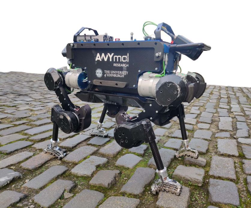
2                                                  IEEE ROBOTICS AND AUTOMATION LETTERS. PREPRINT VERSION. ACCEPTED FEBRUARY, 2021

fashion. Crocoddyl [8] improves the computation speed further         1) We propose to formulate foothold planning as a QP
more. A frequency-aware MPC is proposed in [9] to deal with              problem subject to LIPM dynamics, which can be solved
the bandwidth limitation problem for real hardware. In those             within the control cycle of 2.5 ms. Running re-planning
four works, the contact planning problem has been decoupled              at high frequency allows the robot to be responsive
from the whole-body motion planning problem.                             to disturbances and control commands. The higher the
   Footstep optimization on biped robots has been proposed in            updating frequency of the MPC, the better the reactivity
[10] [11]. An underactuated linear inverted pendulum model               achieved by the robot.
(LIPM) has been used to formulate the footstep optimization           2) We use unconstrained infinite-horizon LQR to generate
problem. The idea has been extended and generalized to both              optimal gains for base control in order to improve the
biped and quadruped robots in our previous work [12]. In                 robustness of the controller and cope with underac-
this work, we realize real-time footstep optimization that can           tuation. Meanwhile, we inherit the advantage of our
be executed in a MPC fashion and test it on the hardware                 previous projected inverse dynamic framework to satisfy
ANYmal.                                                                  the inequality constraints in an orthogonal subspace,
                                                                         which is different to the purely QP-based controllers
B. Related control methods                                               [13][14][15].
   In recent years, there has been a convergence among
legged robot researchers to formulate the control problem           D. Paper organization
as a Quadratic Program (QP) with constraints. The problem              The paper is organized in accordance with the hierarchical
can be further decomposed into hierarchies to coordinate            structure of the whole system, which is shown in Fig. 2. Given
multiple tasks within whole-body control [13][14][15]. These        the desired velocity, the foothold planner plans future footsteps
optimization-based controllers usually rely on manually tuned       based on the current robot state which is explained in Section
diagonal feedback gain matrices. Also, these controllers only       II. Section III describes the derivation of the LQR for base
compute the best commands for the next control cycle, and           control. Simulations, experiments and discussions are given in
therefore are not suitable for dynamic gaits with underac-          Section IV. Finally, Section V draws the relevant conclusions.
tuation. Classical optimal control theory, such as LQR, can
consider long or even infinite time horizons and generate op-
                                                                                      II. M OTION GENERATION
timal non-diagonial gain matrices exploiting dynamic coupling
effects which benefit underactuated systems such as a cart-pole        When considering dynamic gaits such as trotting, two
[16].                                                               contact points cannot constrain all six degrees of freedom
   Classical LQR does not consider any constraints except           (DOF) of the floating base. The system becomes underactuated
system dynamics. However, for legged robots, we have to             as one DOF around the support line is not directly controlled.
satisfy inequality constraints such as torque limits and friction   Researchers have been using the LIPM as an abstract model
cones on contact feet. The works [17][18] proposed to use the       for balance control in this situation. The Centre of Mass (CoM)
classical LQR controller for bipedal walking, but inequality        position and velocity can be predicted by solving the forward
constraints were not enforced. In this paper, we propose an         dynamics of the passive inverted pendulum. In order to keep
LQR controller for dynamic gait control under the framework         long term balance, the next ZMP point has to be carefully
of projected inverse dynamics [19][20]. Projected inverse           selected to capture the falling CoM. For trotting, the ZMP
dynamic control enables us to control motion in a constraint-       point always lies on the support line formed by the supporting
free subspace while satisfying inequality constraints in an         leg pair. As a result, the footholds optimization problem can
orthogonal subspace. In our previous work, we used Cartesian        be transformed to a ZMP optimization problem.
impedance controllers within the constraint-free subspace to
control both the base and swing legs during static walking          A. MPC formulation
of a quadruped robot. Here, we use LQR in the constraint-
free subspace to replace the Cartesian impedance controller           The dynamics of the linear inverted pendulum is as follows:
for base motion control and to handle the underactuation in                                    g
                                                                                  ẍCoM =          (xCoM − px )
the trotting gait.                                                                           zCoM
                                                                                               g                              (1)
                                                                                  ÿCoM =          (yCoM − py )
                                                                                             zCoM
C. Contributions
                                                                    where xCoM , yCoM and zCoM are the CoM position coor-
   This paper focuses on improving the robustness of dynamic
                                                                    dinates, px and py are the coordinates of ZMP, g represents
quadrupedal gaits. The trotting and pacing gaits of a quadruped
                                                                    the acceleration of gravity. Considering zCoM as constant, the
robot will be studied and demonstrated in simulations and
                                                                    dynamics become linear and result in the following solution:
real experiments (see Fig. 1). The main contributions lie in
the computation speed of the MPC and the optimal feedback                         xCoM (t) = A(t)x0CoM + B(t)px
control. As an additional contribution, our approach is shown                                     0
                                                                                                                                 (2)
                                                                                  yCoM (t) = A(t)yCoM + B(t)py
to be valid both with the default spherical feet and the adaptive
feet [21] with flexible soles. The main contributions are listed    where xCoM       =     [xCoM ẋCoM ]⊤ , yCoM       =
as follows:                                                          [yCoM ẏCoM ] , are the state vectors, and x0CoM and
                                                                                  ⊤
XIN et al.: ROBUST FOOTSTEP PLANNING AND LQR CONTROL FOR DYNAMIC QUADRUPEDAL LOCOMOTION 3
Foot trajectory Swing leg
generator impedance control Constraint Space
Footstep planner QP optimization
(MPC) Constraint-free Space s.t. ineq constraints
Base trajectory Base motion
generator LQR control
State estimator
Fig. 2. Control framework block diagram. All the modules are running at 400 Hz. The joystick sends desired walking velocities. The MPC generates desired
ZMPs. The ZMPs are mapped to foot placements which generate swing foot trajectories by interpolation. The desired base trajectory is generated based on
desired ZMPs. An LQR and two impedance controllers are employed to track desired base trajectory and swing foot trajectories in the constraint-free space.
Constraints, such as torque limits and friction cone, are satisfied in the constraint space.
0
yCoM are the initial state vectors. A(t) and B(t) are defined where ẋCoMd is the desired CoM velocity in the x direction,
as Qi and Ri are weight factors. The cost function for the y
cosh(ωt) ω −1 sinh(ωt)
A(t) = (3) direction has the same form as Eq. (8). The MPC is formulated
ω sinh(ωt) cosh(ωt) as a QP minimizing Eq. (8) subject to Eq. (5) and Eq. (7).
1 − cosh(ωt)
Solving the QP results in the optimal ZMPs for the future N
B(t) = (4) steps p∗x = [p∗x1 p∗x2 . . . p∗xN ]⊤ .
−ω sinh(ωt)
p Similarly, solving another QP for y direction yields the co-
while ω = g/zCoM . ordinate p∗y = [p∗y1 p∗y2 . . . p∗yN ]⊤ for the optimal ZMPs
For a periodic trotting gait with fixed swing duration Ts , in this direction. It should be noted that the cost function for
assuming instant switching between single support phases, the y direction is slightly different to Eq. (8), which is as follows
states of N future steps along x direction can be predicted N
given step duration Tsi
X 1
[Qi (ẏCoMi − ẏCoMd )2 + Ri (pyi − pyi−1 − s(−1)i ry )2 ]
2
xCoM1 = A(Ts1 )xCoM0 + B(Ts1 )px1 i=1
(9)
xCoM2 = A(Ts2 )xCoM1 + B(Ts2 )px2 where ry is a constant distance between right and left ZMPs.
.. (5) ry 6= 0 for pacing gait to avoid self-collision while ry = 0
.
for trotting gait. s indicates the support phase the robot is in,
xCoMN = A(TsN )xCoMN −1 + B(TsN )pxN s = 1 for left support and s = −1 for right support.
where xCoM0 is the state at the moment of first touchdown, We only use the first pair p∗1 = (p∗x1 p∗y1 ) to generate the
which can be computed from swing trajectory. Since the MPC is running in the same loop
of controller, the position p∗1 = (p∗x1 p∗y1 ) keeps updating
xCoM0 = A(t0 )x0CoM + B(t0 )px0 (6) during a swing phase given the updated CoM state (x0CoM
0
where t0 is the remaining period of the current swing phase. yCoM ) and desired CoM velocity (ẋCoMd ẏCoMd ).
x0CoM and px0 are the current CoM state and ZMP location
given by the state estimator which also runs at 400 Hz. B. Reference trajectories of trotting gait
Also, considering the kinematic limits of the swing feet, the This section explains the algorithms to generate the desired
following inequality constraints are enforced: trajectories of swing feet and the CoM for trotting gait based
on the results of the MPC. The MPC provides the optimal
px 0 − d 1 0 ··· 0 0 px 1 px 0 + d ZMP that should be on the line connecting the next pair of
−d −1 1 ··· 00 px 2 d support legs. We choose the ZMP to be the middle point of
.. .. .. .. .. .. ≤ ..
.. the support line for trotting gait. We keep the distance from
. ≤ . . . ..
. .
−d 0 0 · · · 1 0 pxN −1
d the ZMP to each support foot location to be a fixed value r.
−d 0 0 · · · −1 1 px N d Then we use the following equations to compute the desired
(7) footholds when the feet are swinging (in Fig. 3):
where d is a constant value derived from kinematic reacha- ∗
pLF
bility relative to the stance feet. Additionally, Eq. (7) can also x px 1 cos(θ0 + ∆θ)
LF : = ∗ +r
be used to avoid stepping into unfeasible pitches on the ground pLF
y p sin(θ0 + ∆θ)
y∗1
by redefining d.
RH
px px 1 − cos(θ0 + ∆θ)
The state along y direction has the same evolution as shown RH : = ∗ +r
pRH
y p − sin(θ0 + ∆θ)
in Eq. (5). Regarding ZMPs as the system inputs, we define RF ∗y1 (10)
px px 1 cos(θ0 − ∆θ)
the cost function of the MPC as follows RF : = + r
pRF p∗ − sin(θ0 − ∆θ)
N
1 yLH y∗1
px px 1 − cos(θ0 − ∆θ)
X
[Qi (ẋCoMi − ẋCoMd )2 + Ri (pxi − pxi−1 )2 ] (8) LH : = + r
i=1
2 pLH
y p∗y1 sin(θ0 − ∆θ)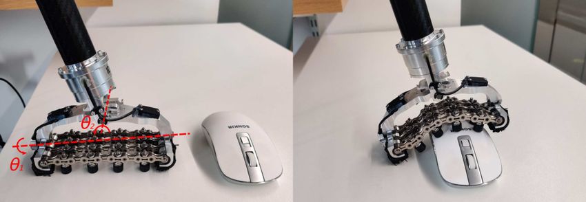
4                                                           IEEE ROBOTICS AND AUTOMATION LETTERS. PREPRINT VERSION. ACCEPTED FEBRUARY, 2021

                                                                                  The dynamics of a legged robot can be projected into
                                                                                two orthogonal subspaces by using the projection matrix
                                                                                P = I − J+c Jc [22][23] as follows:
                                                                                  Constraint-free space:
                                                                                                      PMq̈ + Ph = PSτ                       (11)
                                                                                  Constraint space:
                                                                                           (I − P)(Mq̈ + h) = (I − P)Sτ + J⊤      c λc      (12)
                                                                                                                ⊤
                                                                                   where q = I xb q⊤
                                                                                                  ⊤
                                                                                                                  ∈ SE(3) × Rn , where I xb ∈

                                                                                                           j
                                                                                SE(3) denotes the floating base’s position and orientation with
                                                                                respect to a fixed inertia frame I, meanwhile qj ∈ Rn denotes
                                                                                the vector of actuated joint positions. Also, we define the gen-
                                                                                                                                     ⊤
                                                                                eralized velocity vector as q̇ = I vb⊤ B ω ⊤     q̇⊤    ∈ R6+n ,

                                                                                                                              b    j
                                                                                                  3                  3
                                                                                where I vb ∈ R and B ω b ∈ R are the linear and angular
                                                                                velocities of the base with respect to the inertia frame ex-
                                                                                pressed respectively in the I and B frame which is attached
Fig. 3. Geometrical relationship between footholds and ZMPs. We assign the      on the floating base. M ∈ R(n+6)×(n+6) is the inertia matrix,
current ZMP (p0 ) to be the middle point of the support line at the touchdown
moment. The desired footholds (p∗LF , p∗RH ) are calculated from the desired    h ∈ Rn+6 is the generalized vector containing Coriolis,
ZMP (p∗1 ) and two foot pair parameters r and θ. r determines the distance      centrifugal and gravitational effects, τ ∈ Rn+6 is the vector
between the foot pair and θ determines the orientation of the foot pair with    of torques, Jc ∈ R3k×(n+6) is the constraint Jacobian that
respect to the robot heading direction. Nominal values are used for these two
parameters. If there is a given steering command ωz , the orientation can be    describes 3k constraints, k denotes the number of contact
updated θ = θ0 + ωz · dt.                                                       points accounting foot contact and body contact, λc ∈ R3k
                                                                                are constraint forces acting on contact points, and

                                                                                                               0       06×n
where LF, RH, RF and LH are the abbreviations for left-fore,                                          S = 6×6                               (13)
                                                                                                               0n×6 In×n
right-hind, right-fore and left-hind feet. θ0 is a constant angle
measured in the default configuration while ∆θ is the rotation                  is the selection matrix with n dimensional identity matrix
command sent by the users. For pacing gait, θ0 = 0.                             In×n .
   Here we do not tackle the height changing issue. We use                         Note that Eq. (11) together with Eq. (12) provides the whole
the current height of support feet to be the desired height                     system dynamics. The sum of the torque commands generated
of desired footholds for swing feet. The peak height during                     in the two subspaces will be the final command sent to the
swing is a fixed relative offset. This technique has to be                      motors as shown in Fig. 2. In this paper, we focus on trajectory
adapted for some tasks such as climbing stairs. However the                     tracking control in the constraint-free subspace. We refer to our
robustness of the planner and controller can handle slightly                    previous paper [20] for the inequality constraint satisfaction
rough terrains, as we demonstrate through experiments. After                    in the constraint subspace. The swing legs are controlled by
determining the desired footholds, we use cubic splines to                      impedance controllers proposed in our former paper [20]. In
interpolate the trajectories between the initial foot positions                 this paper, we propose to replace the impedance controller
and desired footholds for the swing feet, and feed the one                      for base control with an LQR controller, benefiting from
forward time step positions, velocities and accelerations to the                the optimal gain matrix instead of the hand-tuned diagonal
controller.                                                                     impedance gain matrices.
   The desired positions and velocities for CoM are determined                     The similar works of [17][18] did not enforce any inequality
by the LIPM, i.e., Eq. (2) where the initial states x0CoM and                   constraints with the classical LQR controller. The advantage
  0
yCoM   are updating with 400 Hz as well. Setting the variable                   of using projected inverse dynamics is that we can satisfy hard
t in Eq. (2) to be a constant value t = 2.5 ms results in                       constraints, such as torque limits and friction cone constraints,
the desired CoM positions and velocities along x and y for                      in the constraint space by solving a QP as shown in Fig. 2,
controller. We set the desired height of CoM to be a constant                   in case the LQR controller and impedance controller generate
value with respect to the average height of the support feet.                   torque commands that violate those inequality constraints.

                                                                                A. Linearization in Cartesian space
                  III. LQR FOR BASE CONTROL
                                                                                  Based on Eq. (11), we derive the forward dynamics
   We continue to use our projected inverse dynamic control                                 q̈ = M−1                −1
                                                                                                  c (−Ph + Ṗq̇) + Mc PSτ                   (14)
framework [20] as it allows us to focus on designing trajectory
tracking controllers without considering physical constraints.                   where Mc = PM + I − P is called constraint inertia matrix
The physical constraints will be satisfied in an orthogonal                     [22]. Eq.
                                                                                        (14) could
                                                                                                ⊤ be linearized with respect to the full state
subspace. This framework gives us the opportunity to use the                    vector q⊤ q̇⊤ . However, the resulting linearized system
classical LQR without any adaptation.                                           would not be controllable as the corresponding controllability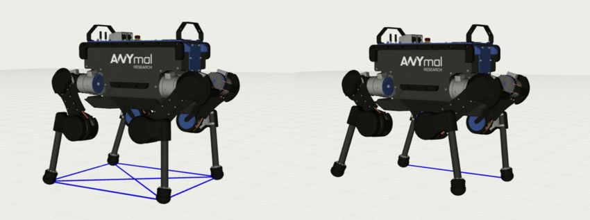
XIN et al.: ROBUST FOOTSTEP PLANNING AND LQR CONTROL FOR DYNAMIC QUADRUPEDAL LOCOMOTION                                                                                                                5

matrix is not full rank. Instead of resorting to one more                 around current configuration in order to improve computation
projection as done in [17], we linearize the dynamics in the              accuracy if the computation is fast enough.
Cartesian space to control only the base states rather than all              In practice, we increase the weights in R of Eq. (22) for
the states of a whole robot.                                              swing legs, relying more on the support legs for base control.
   Just using a selection matrix, we can derive the forward               Otherwise, the torque commands of Eq. (23) can affect the
dynamics with respect to I xb                                             tracking of swing trajectories too much.
                                                                             In addition, the motion planner in Section II feeds the
 ẍb = Jb M−1                      −1
            c (−Ph + Ṗq̇) + Jb Mc PSτ = f (I xb , ẋb , τ )              desired CoM trajectory to the controllers, whereas the LQR
                                                       ⊤ (15)            controller controls the base pose. In theory, we should replace
where Jb = [I6×6 06×n ]6×(n+6) , ẋb = I vb⊤ B ω ⊤

                                                         .
                                                    b                     I xb with xCoM in Eqs. (11)(12) and transform the dynamic
   By using Euler angles for the orientation in I xb , we can             equations to be with respect to CoM variables as in [25]. Then
define the state vector as                                                the LQR controller will directly track the desired CoM trajec-

                              x                                           tory. In this paper, we approximately consider the translation of
                        X= I b                             (16)
                             ẋb 12×1                                     base along x and y aligned with CoM since the base dominates
                                                                          the mass of the whole robot.
 We linearize Eq. (15) to state space dynamics around a con-
figuration (q0 , q̇0 , τ 0 ) where τ 0 is the gravity compensation
                                                                                                                              IV. VALIDATIONS
torques, yielding
                           Ẋ = Ab0 X + Bb0 τ                 (17)           We use a torque controllable quadruped robot ANYmal
                                                                          made by ANYbotics to conduct our experiments. The onboard
Eq. (17) is detailed as                                                   computer has an Intel 4th generation (HaswellULT) i7-4600U

             ẋb        0         I
                                                                     (1.4 GHz-2.1 GHz) processor and two HX316LS9IBK2/16
                                             I xb         0
                  =                                     +      τ   (18)   DDR3L memory cards. The robot weights approximately
             ẍb      A21        A22         ẋb          B2
                                                                          35 kg and has 12 joints actuated by Series Elastic Actuators
where A21 , A22 and B2 are defined as                                     (SEAs) with maximum torque of 40 N · m. The real-time
                           ∂f (I xb , ẋb , τ )                           control cycle is 2.5 ms. The control software is developed
                A21 =                           |q0 ,q̇0 ,τ 0      (19)   based on Robot Operating System 1 (ROS 1). We use the
                                ∂ I xb
                                                                          dynamic modeling library Pinocchio [26] to perform the model
                             ∂f (I xb , ẋb , τ )                         linearization of Section III. An active set method based QP
                  A22 =                           |q0 ,q̇0         (20)
                                   ∂ ẋb                                  solver provided by ANYbotics is used to solve the QPs for the
                                                                          MPC planner and the controller. A video of the experimental
                   ∂f (I xb , ẋb , τ )                                   results can be found at: https://youtu.be/khP6PQ9xuso.
            B2 =                        = Jb M−1
                                              c PS|q0   (21)
                          ∂τ
   For simplicity, we use a central finite difference method              A. Trotting speed
to compute the partial derivatives of Eq. (19) and Eq. (20).
                                                                             We first tested the fastest walking speed when using the
The deviation factor for finite difference we used for the
                                                                          proposed algorithms. Figure 4 shows the recorded speeds
experiments is 1 × 10⁻⁵ .
                                                                          along x direction in real robot experiment and in simulation. In
                                                                          simulation, the robot could stably trot forward with maximum
B. LQR controller                                                         speed 1.2 m/s. On real robot, the maximum speed reached
   We consider Eq. (17) as a linear time-invariant system and             0.6 m/s. The results are reasonable since the trotting gait does
solve the infinite horizon LQR problem to compute the optimal             not have a flying phase. The fact that the real robot cannot
feedback gain matrix K. The cost function to be minimized                 achieve as fast motion as in simulation is also reasonable
is defined as                                                             considering model errors and other uncertainties. Model errors
                      Z ∞                                                 also cause drifting on the real robot which is difficult to
                 J=       (X⊤ QX + τ ⊤ Rτ )dt            (22)             resolve without external control loops. Constant values for
                       0
and the resulting controller for the base control is
                                                                                                     Trotting speed of the real robot                                   Trotting speed in simulation
                                                                                           0.8                                                                1.5
                   τ m2 = K(Xd − X) + τ d                          (23)
                                                                                           0.6
                                                                          Velocity (m/s)

                                                                                                                                             Velocity (m/s)

                                                                                                                                                                1
where Xd is the desired state, τ d is the feedforward term
                                                                                           0.4
derived from inverse dynamics based on the desired state.
                                                                                                                                                              0.5
   We use ADRL Control Toolbox (CT) [24] to solve the                                      0.2
infinite-horizon LQR problem and obtain the K matrix. It
                                                                                             0                                                                  0
should be noted that the linearization is computed in every                                      0                  5                   10                          0         5         10        15
                                                                                                                   t (sec)                                                          t (sec)
control cycle based on the current configuration (q0 , q̇0 , τ 0 ).
The K matrix is updated at 400 Hz, which is different to [18]             Fig. 4. Recorded fastest trotting speeds on real robot and in simulation. The
where they only compute the K matrices corresponding to few               desired velocities are generated from LIPM dynamics, i.e. Eq. (2), which
key configurations. We think linearization should be updated              explains why the reference velocities are not smooth.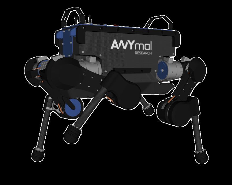
6 IEEE ROBOTICS AND AUTOMATION LETTERS. PREPRINT VERSION. ACCEPTED FEBRUARY, 2021
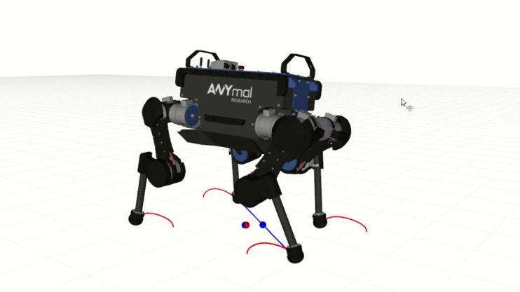
Fig. 5. Footstep and swing trajectory replanning under disturbances. The robot is walking forward and an external force (green arrow) is applied to the base
of the robot. The push results in a sudden change of the CoM position and velocity. The footstep planner uses the updated state to replan the footholds. The
swing trajectories (red lines) are updated accordingly.
0.4 1
0.2
0.5
Velocity (m/s)
Velocity (m/s)
0
-0.2 0
-0.4
-0.5
-0.6
-0.8 -1
0 5 10 15 20 25 0 5 10 15 20 25
t (sec) t (sec)
0.1
0.6
0.4
0
Orientation (rad)
Position (m)
0.2
0 -0.1
-0.2
-0.2
-0.4
-0.3
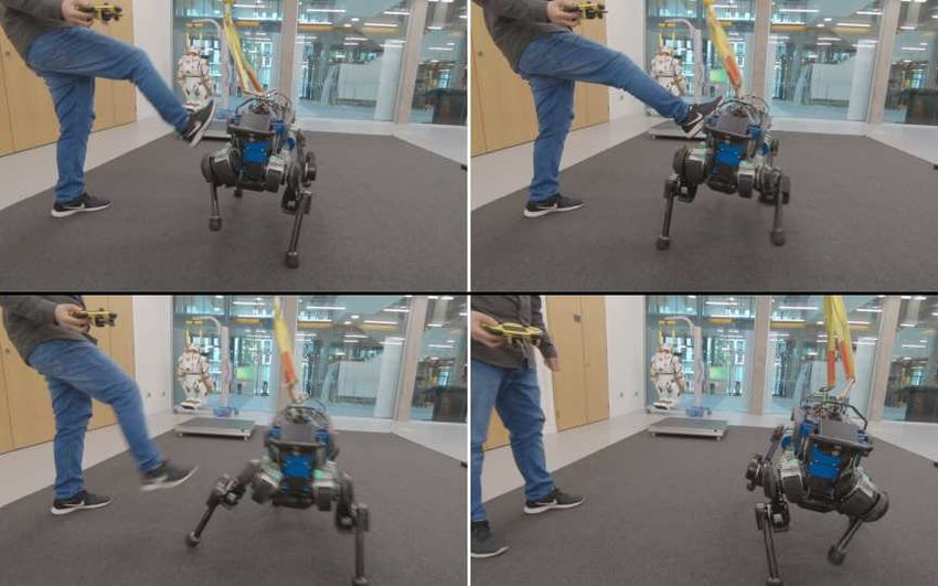
Fig. 6. Kicking the robot during trotting. Benefiting from the 400 Hz MPC 0 5 10 15 20 25 0 5 10 15 20 25
update frequency, the robot can quickly update the optimal footholds to t (sec) t (sec)
recover from disturbances.
Fig. 7. Recorded state when the robot was kicked four times. The desired
Euler angles were 0. The robot was quickly regulated back to normal even
the parameters of the gait planner were employed. They are though the velocity reached −1 m/s after kicking.
Ts = 0.3, zCoM = 0.42, g = −9.8, N = 3, Qi = 1000,
Ri = 1, θ0 = 0.56, r = 0.41. It should be noted that the
prediction number N in the MPC does not need to be as large
as possible with the concern of computation efficiency. We
tested N = 2 ∼ 5, and they showed similar performance.
B. Push recovery
In this subsection, we demonstrate the benefit of high
frequency replanning for disturbance rejection. We first use
simulation to show the replanned footholds and trajectories Fig. 8. Visualization of the gain matrix as computed by the LQR controller
during trotting. The size of the gain matrix is 18 by 12. The first 6 columns
as shown in Fig. 5. The disturbance is added when RF and correspond to the position and orientation while the remaining 6 columns are
LH feet are swinging. The disturbance results in sharp state for velocity control. Off-diagonal gains demonstrate that dynamic coupling
changes. The MPC computed the new footholds after receiving effects may be exploited for control.
the updated state. Figure 6 presents snapshot photos of the
push-recovery experiment on the real robot during trotting
while recorded state data is shown in Fig. 7. The robot was balance. Recently researchers demonstrated that quadruped
kicked four times roughly along the y direction. We can see robots with point feet can stand on two feet to maintain balance
the peak velocity of y reached −1 m/s during the last two [27][28]. Although we did not manage balancing on two feet
kicks, but it was quickly regulated back to normal using one on our robot, we compared the longest period of swing phase
or two steps. The orientation did not change too much after of trotting when using our proposed LQR controller versus
kicking, which also indicates the robustness of the method. the default trotting controller of ANYmal [29]. The longest
swing phase when using LQR is 0.63 s whereas the default
controller only achieved 0.42 s. When the base is controlled
C. Balance control by our previous impedance controller, the longest swing phase
Most of the trotting gait control algorithms rely on quick is 0.4 s. This verifies the improved performance of our LQR
switching of swing and stance phases to achieve dynamic controller in terms of balance control. Figure 8 shows two gain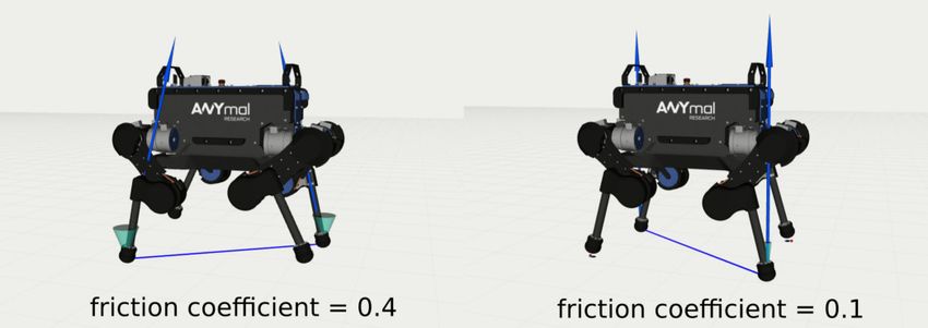
XIN et al.: ROBUST FOOTSTEP PLANNING AND LQR CONTROL FOR DYNAMIC QUADRUPEDAL LOCOMOTION                                                          7

matrices for the two phases of trotting during this experiment.
It should be noted that the gain matrices are updated in
every control cycle (but the changes are small). We can see
that the elements of the first 6 rows are 0 because of the
existence of selection matrix S. The Q12×12 we used in the
experiment was Q = diag(diag(1500)6×6 , diag(1)6×6 ). The
R18×18 was switched depending on the phase. The diagonal
elements corresponding to the two swing legs in R are 10
times larger than the other diagonal elements for stance legs       Fig. 9. The friction cone constraints are satisfied by the controller. The blue
and the base, reducing the efforts of swing legs in balance         arrows represent the actual contact forces while the green cones denote the
control. The elements in R for stance legs and the base we          friction cones.
used in this experiment are 0.03.

D. Trotting on slippery terrains
   The most important advantage of the proposed control
framework compared to similar works [17][18] is that we
can satisfy inequality constraints while using LQR for tra-
jectory tracking. We do not change the classical LQR to be
a constrained LQR. By contrast, using the projected inverse
dynamic control allows us to satisfy inequality constraints in
the constraint subspace. The LQR controller only serves as a        Fig. 10. A base shifting motion is needed to transit from trotting to pacing.
trajectory tracking controller and does not need to consider the
inequality constraints. The QP optimization in the constraint
subspace plays the role of trading off different constraints. For   Compared to the traditional sphere feet, the adaptive feet
example, as we have shown in our previous paper [20] for            have larger contact surface. Those features will benefit the
static gait, trajectory tracking performance will be sacrificed     traversability of rough terrains with rocks, loose gravel and
to prevent slipping if torque commands for trajectory tracking      rubble by enlarging the contact surfaces with ground. We per-
generate contact forces beyond the friction cones. Here we          formed experiments in trotting locomotion on rough terrains
demonstrate that our proposed controller can satisfy friction       outside our lab as shown in Fig. 12. It should be noted that
cone constraints for dynamic gaits as well. Figure 9 shows          our controller did not take the two DOF (one DOF less than
the controller can keep the contact forces within the friction      the case with a spherical foot) passive ankle into account.
cone after reducing the friction coefficient to match the actual    The model errors caused by the adaptive feet were treated as
friction coefficient of the terrain. The smallest friction coef-    disturbances by the controller, where the success of the tests
ficient we achieved in simulation for trotting in spot on flat      shows the robustness of our controller.
terrain is 0.07. However it is difficult to trot on such slippery
terrain because the trajectory tracking is quite poor in this
situation.                                                                                   V. CONCLUSIONS

E. Transition from trotting to pacing                                  This paper presents a full control framework for dynamic
                                                                    gaits where all the modules are running with the same fre-
   Pacing gait is a more dynamic gait compared to trotting
                                                                    quency. The robustness of the dynamic walking is improved
since the CoM is always off the supporting line. The difference
                                                                    significantly by two factors. The first factor is the MPC plan-
between trotting and pacing in terms of the MPC formulation
                                                                    ner, which mostly contributes to rejecting large disturbances,
is that there will be a constant offset ry between pyi and
                                                                    such as kicking the robot, because the MPC uses footsteps
pyi−1 (see Fig. 10) in the cost function Eq. (9) in order to
                                                                    to regulate the state of the robot. The second factor is the
avoid conflicts of the right and left feet. In our experiment,
                                                                    LQR controller for balancing control, which also undertakes
we specified a transition motion of shifting the base to a side
                                                                    the duty of trajectory tracking. The method is general and
to start pacing. We can also remove this transition motion by
                                                                    shown to able to work both with spherical and adaptive
reducing the gait period or reducing the distance between left
                                                                    feet. The latter were seen to reduce the slipping chance
and right feet. The gait period in this experiment was 0.44 s
                                                                    on rough terrains. The outdoor experiments demonstrate the
with ry = 0.08 m. On the controller side, we used the same
                                                                    robustness of locomotion after adopting the proposed methods
Q and R for trotting and pacing.
                                                                    and assembling the adaptive feet.
                                                                       Future work will focus on adapting the current planner to
F. Outdoor test with adaptive feet                                  consider terrain information to handle large slopes and stairs.
  In this subsection, we test the versatility of our approach       Also, the new feet can be used to measure the local inclination
with adaptive feet SoftFoot-Q [21] in outdoor environments.         of the ground which can improve the accuracy of the terrain
Figure 11 shows a typical case of the adaptive feature.             information, similar to [30].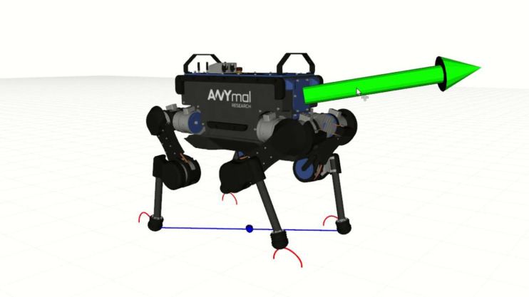
8                                                               IEEE ROBOTICS AND AUTOMATION LETTERS. PREPRINT VERSION. ACCEPTED FEBRUARY, 2021

                                                                                    [10] S. Faraji, S. Pouya, C. G. Atkeson, and A. J. Ijspeert, “Versatile and
                                                                                         robust 3d walking with a simulated humanoid robot (atlas): A model
                                                                                         predictive control approach,” in Proc. IEEE Int. Conf. Robot. Autom.,
                                                                                         2014, pp. 1943–1950.
                                                                                    [11] S. Feng, X. Xinjilefu, C. G. Atkeson, and J. Kim, “Robust dynamic
                                                                                         walking using online foot step optimization,” in Proc. IEEE Int. Conf.
                                                                                         Intell. Robots Syst., 2016, pp. 5373–5378.
                                                                                    [12] S. Xin, R. Orsolino, and N. G. Tsagarakis, “Online relative footstep
                                                                                         optimization for legged robots dynamic walking using discrete-time
                                                                                         model predictive control.” in Proc. IEEE Int. Conf. Intell. Robots Syst.,
                                                                                         2019, pp. 513–520.
Fig. 11. The SoftFoot-Q, an adaptive foot for quadrupeds. θ1 and θ2 indicate        [13] L. Saab, O. E. Ramos, F. Keith, N. Mansard, P. Soueres, and J. Y.
the passive joints of the ankle.                                                         Fourquet, “Dynamic whole-body motion generation under rigid contacts
                                                                                         and other unilateral constraints,” IEEE Trans. Robot., vol. 29, no. 2, pp.
                                                                                         346–362, 2013.
                                                                                    [14] A. Del Prete, F. Nori, G. Metta, and L. Natale, “Prioritized motion–
                                                                                         force control of constrained fully-actuated robots:task space inverse
                                                                                         dynamics,” Robotics and Autonomous Systems, vol. 63, pp. 150–157,
                                                                                         2015.
                                                                                    [15] A. Herzog, N. Rotella, S. Mason, F. Grimminger, S. Schaal, and
                                                                                         L. Righetti, “Momentum control with hierarchical inverse dynamics on
                                                                                         a torque-controlled humanoid,” Autonomous Robots, vol. 40, no. 3, pp.
                                                                                         473–491, 2016.
                                                                                    [16] P. Reist and R. Tedrake, “Simulation-based lqr-trees with input and state
                                                                                         constraints,” in Proc. IEEE Int. Conf. Robot. Autom., 2010, pp. 5504–
                                                                                         5510.
                                                                                    [17] S. Mason, L. Righetti, and S. Schaal, “Full dynamics lqr control of a
                                                                                         humanoid robot: An experimental study on balancing and squatting,” in
                                                                                         Proc. IEEE Int. Conf. Humanoid Robots, 2014, pp. 374–379.
                                                                                    [18] S. Mason, N. Rotella, S. Schaal, and L. Righetti, “Balancing and walking
                                                                                         using full dynamics lqr control with contact constraints,” in Proc. IEEE
Fig. 12. Trotting out of the lab with adaptive feet on rubble terrain.                   Int. Conf. Humanoid Robots, 2016, pp. 63–68.
                                                                                    [19] G. Xin, H.-C. Lin, J. Smith, O. Cebe, and M. Mistry, “A model-
                                                                                         based hierarchical controller for legged systems subject to external
                                                                                         disturbances,” in Proc. IEEE Int. Conf. Robot. Autom., 2018, pp. 4375–
                         ACKNOWLEDGMENT                                                  4382.
                                                                                    [20] G. Xin, W. Wolfslag, H.-C. Lin, C. Tiseo, and M. Mistry, “An
   The authors would like to thank Dr. Quentin Rouxel and Dr.                            optimization-based locomotion controller for quadruped robots leverag-
Carlos Mastalli for introduction on using the Pinocchio rigid                            ing cartesian impedance control,” Frontiers in Robotics and AI, vol. 7,
body dynamics library. The authors also would like to thank                              p. 48, 2020.
                                                                                    [21] M. G. Catalano, M. J. Pollayil, G. Grioli, G. Valsecchi, H. Kolvenbach,
the editor and reviewers for their useful comments.                                      M. Hutter, A. Bicchi, and M. Garabini, “Adaptive Feet for Quadrupedal
                                                                                         Walkers,” IEEE Trans. Robot., 2020, [Under Review]. [Online].
                                 R EFERENCES                                             Available: https://www.dropbox.com/s/84ry3we72c7kt6s/adaptive feet
                                                                                         preprint.pdf
    [1] A. W. Winkler, F. Farshidian, D. Pardo, M. Neunert, and J. Buchli,          [22] F. Aghili, “A unified approach for inverse and direct dynamics of
        “Fast trajectory optimization for legged robots using vertex-based zmp           constrained multibody systems based on linear projection operator:
        constraints,” IEEE Robot. Autom. Lett., vol. 2, no. 4, pp. 2201–2208,            Applications to control and simulation,” IEEE Trans. Robot., vol. 21,
        2017.                                                                            no. 5, pp. 834–849, 2005.
    [2] A. W. Winkler, C. D. Bellicoso, M. Hutter, and J. Buchli, “Gait and         [23] M. Mistry and L. Righetti, “Operational space control of constrained and
        trajectory optimization for legged systems through phase-based end-              underactuated systems,” Robotics: Science and systems VII, pp. 225–232,
        effector parameterization,” IEEE Robot. Autom. Lett., vol. 3, no. 3, pp.         2012.
        1560–1567, 2018.                                                            [24] M. Giftthaler, M. Neunert, M. Stäuble, and J. Buchli, “The control
    [3] J. Di Carlo, P. M. Wensing, B. Katz, G. Bledt, and S. Kim, “Dynamic              toolbox an open-source c++ library for robotics, optimal and model
        locomotion in the mit cheetah 3 through convex model-predictive                  predictive control,” 2018 IEEE SIMPAR, pp. 123–129, 2018.
        control,” in Proc. IEEE Int. Conf. Intell. Robots Syst., 2018, pp. 1–9.     [25] B. Henze, M. A. Roa, and C. Ott, “Passivity-based whole-body balancing
    [4] D. Kim, J. Di Carlo, B. Katz, G. Bledt, and S. Kim, “Highly dynamic              for torque-controlled humanoid robots in multi-contact scenarios,” Int.
        quadruped locomotion via whole-body impulse control and model                    J. Robotics Res., vol. 35, no. 12, pp. 1522–1543, 2016.
        predictive control,” arXiv preprint arXiv:1909.06586, 2019.                 [26] J. Carpentier, G. Saurel, G. Buondonno, J. Mirabel, F. Lamiraux,
    [5] O. Cebe, C. Tiseo, G. Xin, H.-c. Lin, J. Smith, and M. Mistry, “Online           O. Stasse, and N. Mansard, “The pinocchio c++ library – a fast and
        dynamic trajectory optimization and control for a quadrupedrobot,”               flexible implementation of rigid body dynamics algorithms and their
        arXiv preprint arXiv:2008.12687, 2020.                                           analytical derivatives,” in IEEE International Symposium on System
    [6] J. Koenemann, A. Del Prete, Y. Tassa, E. Todorov, O. Stasse, M. Ben-             Integrations (SII), 2019.
        newitz, and N. Mansard, “Whole-body model-predictive control applied        [27] M. Chignoli and P. M. Wensing, “Variational-based optimal control of
        to the hrp-2 humanoid,” in Proc. IEEE Int. Conf. Intell. Robots Syst.,           underactuated balancing for dynamic quadrupeds,” IEEE Access, vol. 8,
        2015, pp. 3346–3351.                                                             pp. 49 785–49 797, 2020.
    [7] M. Bjelonic, R. Grandia, O. Harley, C. Galliard, S. Zimmermann, and         [28] C. Gonzalez, V. Barasuol, M. Frigerio, R. Featherstone, D. G. Caldwell,
        M. Hutter, “Whole-body mpc and online gait sequence generation for               and C. Semini, “Line walking and balancing for legged robots with point
        wheeled-legged robots,” arXiv preprint arXiv:2010.06322, 2020.                   feet,” arXiv preprint arXiv:2007.01087, 2020.
    [8] C. Mastalli, R. Budhiraja, W. Merkt, G. Saurel, B. Hammoud,                 [29] C. Gehring, S. Coros, M. Hutter, M. Bloesch, M. A. Hoepflinger, and
        M. Naveau, J. Carpentier, L. Righetti, S. Vijayakumar, and N. Mansard,           R. Siegwart, “Control of dynamic gaits for a quadrupedal robot,” in
        “Crocoddyl: An efficient and versatile framework for multi-contact               Proc. IEEE Int. Conf. Robot. Autom., 2013, pp. 3287–3292.
        optimal control,” in Proc. IEEE Int. Conf. Robot. Autom., 2020, pp.         [30] G. Valsecchi, R. Grandia, and M. Hutter, “Quadrupedal locomotion on
        2536–2542.                                                                       uneven terrain with sensorized feet,” IEEE Robot. Autom. Lett., vol. 5,
    [9] R. Grandia, F. Farshidian, R. Ranftl, and M. Hutter, “Feedback mpc for           no. 2, pp. 1548–1555, 2020.
        torque-controlled legged robots,” in Proc. IEEE Int. Conf. Intell. Robots
        Syst., 2019, pp. 4730–4737.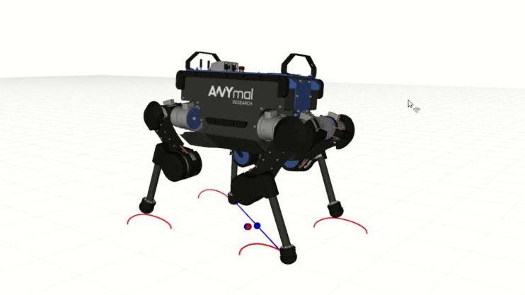
You can also read