Controlling a CyberOctopus Soft Arm with Muscle-like Actuation
←
→
Page content transcription
If your browser does not render page correctly, please read the page content below
Controlling a CyberOctopus Soft Arm with Muscle-like Actuation
                                                               Heng-Sheng Chang1,2 , Udit Halder2 , Ekaterina Gribkova3 , Arman Tekinalp1 ,
                                                                        Noel Naughton1 , Mattia Gazzola1,4,5 , Prashant G. Mehta1,2,3

                                           Abstract— This paper presents an application of the energy              we have worked closely with the biologists on the team
                                        shaping methodology to control a flexible, elastic Cosserat                to incorporate anatomically correct muscular architecture
                                        rod model of a single octopus arm. The novel contributions                 of longitudinal, transverse, and oblique muscles in octopus
                                        of this work are two-fold: (i) a control-oriented modeling of
                                        the anatomically realistic internal muscular architecture of an            arms [6]–[9].
                                        octopus arm; and (ii) the integration of these muscle models into             From a control theoretic perspective of energy shaping,
arXiv:2010.03368v2 [cs.RO] 1 Apr 2021

                                        the energy shaping control methodology. The control-oriented               the muscle constraints limit the energy landscape that can
                                        modeling takes inspiration in equal parts from theories of                 possibly be ‘shaped’ by the use of control. In the energy
                                        nonlinear elasticity and energy shaping control. By introducing
                                                                                                                   shaping literature, a mathematical characterization of achiev-
                                        a stored energy function for muscles, the difficulties associated
                                        with explicitly solving the matching conditions of the energy              able energy is given in terms of the so-called matching
                                        shaping methodology are avoided. The overall control design                conditions [10], [11]. However, solving these conditions is
                                        problem is posed as a bilevel optimization problem. Its solution           a formidable task [12], [13]. Our preliminary attempts at
                                        is obtained through iterative algorithms. The methodology                  directly applying the energy shaping methodology ran into
                                        is numerically implemented and demonstrated in a full-scale
                                                                                                                   this challenging problem.
                                        dynamic simulation environment Elastica. Two bio-inspired
                                        numerical experiments involving the control of octopus arms                   The key idea of this paper is to isolate and model the
                                        are reported.                                                              conservative parts of the muscle forces using the formalism
                                           Index Terms— Cosserat rod, Hamiltonian systems, energy-                 of stored energy function borrowed from nonlinear elas-
                                        shaping control, soft robotics, octopus                                    ticity [14], [15]. This has an advantage in the sense that
                                                                                                                   it circumvents the need to explicitly solve the matching
                                                                I. I NTRODUCTION                                   conditions. The specific contributions are as follows:
                                           Research interest in soft robotic manipulators comes from               1. Control-oriented modeling of muscles: Muscles provide
                                        the potential capability of soft manipulators to perform                   internal (tension) forces. The modeling of a muscle is based
                                        complex tasks in an unstructured environment and safely                    upon the Hill’s model [16]–[19] that prescribes a force-length
                                        around humans [1]–[3]. Bio-inspiration is often provided by                (conservative) and a force-velocity (dissipative) relationship
                                        soft-bodied creatures, such as octopuses, that have evolved                for an activated muscle. Our contribution is to model the
                                        to solve complex motion control problems like reaching,                    conservative muscle force in terms of the stored energy
                                        grasping, fetching, crawling, or swimming. The exceptional                 function of nonlinear elasticity. For the longitudinal and
                                        coordination abilities of these marine animals have naturally              transverse muscles of an octopus arm, explicit expressions
                                        motivated efforts to gain a deeper understanding of the                    of the stored energy function are derived based upon first
                                        biophysical principles underlying their distributed neuromus-              principle modeling and published force-length characteris-
                                        cular control.                                                             tics.
                                           This paper is a continuation of our prior work [4] where                   The inspiration for such a model comes in equal part from
                                        an energy shaping methodology was introduced for a fully                   the hyperelastic rod theory and from the energy shaping
                                        actuated Cosserat rod model of an octopus arm. The method-                 control theory. Similar to the elasticity in Cosserat rod
                                        ology was applied to solve motion problems, e.g. reaching                  theory [14], the control terms on account of muscles are
                                        and grasping, inspired by experiments involving octopus                    modeled as Hamiltonian vector fields.
                                        arms [5]. A major limitation of this prior work was that
                                        the muscle actuator constraints were ignored. In this paper,               2. Application of energy shaping for muscular arm
                                                                                                                   control: The control problem is to activate the muscles to
                                          We gratefully acknowledge financial support from ONR MURI N00014-        solve motion control tasks, e.g. reaching and grasping. The
                                        19-1-2373, NSF/USDA #2019-67021-28989, and NSF EFRI C3 SoRo                control problem is posed and solved as a bilevel optimization
                                        #1830881. We also acknowledge computing resources provided by the
                                        Blue Waters project (OCI- 0725070, ACI-1238993), a joint effort of the     problem. The upper level problem seeks to find the optimal
                                        University of Illinois at Urbana-Champaign and its National Center for     muscle activation subject to the equilibrium constraints that
                                        Supercomputing Applications, and the Extreme Science and Engineering       are shown to arise as a result of solving a lower level
                                        Discovery Environment (XSEDE) Stampede2 (ACI-1548562) at the Texas
                                        Advanced Computing Center (TACC) through allocation TG-MCB190004.          optimization problem. For the bilevel optimization problem,
                                          1 Department of Mechanical Science and Engineering, 2 Coordinated        necessary conditions of optimality are derived by an applica-
                                        Science Laboratory, 3 Neuroscience Program, 4 National Center for Super-   tion of the maximum principle of the optimal control theory.
                                        computing Applications, & 5 Carl R. Woese Institute for Genomic Biol-
                                        ogy, University of Illinois at Urbana-Champaign. Corresponding e-mail:     This also leads to iterative algorithms to compute the control.
                                        udit@illinois.edu                                                          Conditions are given for the asymptotic stability of the rod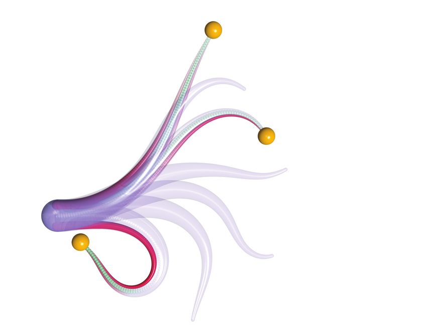
!1#$2&3$34(+451,4&*$                                                    !"#$%&'(()(*+,-'.$/-*0
                                                                                                         '.$/-*0

                                                                     b                                                                s = L0
                                                        s                 a
                                                                              θ
                                          s=0                    r                        rLM
                                                                         ∂s r                                          6'"&'(72"5
                                                                                                                       !"#$%&'"%'()*%+,'
                                                      e2                                                               12$3/4*5/$#,()*%+,'
                                                                                                                       -.,/0*'()*%+,'
                                                            e1           !+#$6-375-8-*9$:;$(-9*$/-*0

Fig. 1: An octopus arm is modeled as a Cosserat rod – (a) a simplified 3D view of the internal musculature, (b) a cross-section
of the arm showing organization of different kinds of muscles, and (c) a 2D model of the arm where we only consider
effects of longitudinal and transverse muscles.

equilibrium obtained using the control.                          L0 . There are two independent coordinates: time t ∈ R and
   The dynamics of the arm together with the muscle ac-          the arc-length coordinate s ∈ [0, L0 ] of the center line. The
tuation model are simulated in the computational platform        configuration of the rod is described by the function
Elastica [20]–[22]. The control methodology is implemented
and demonstrated for reaching and grasping tasks.                                              q(s, t) := (r(s, t), θ(s, t))
   The remainder of this paper is organized as follows. An
anatomical overview of the arm musculature, the planar           where r = (x, y) ∈ R2 denotes the position vector of the
Cosserat rod modeling, and the control objectives appear in      center line, and the angle θ ∈ R defines a material frame
Sec. II. The two main contributions of this paper appear in      spanned by the orthonormal basis {a, b} where (see Fig. 1c)
Sec. III on control-oriented muscle modeling, and in Sec. IV
on application of energy shaping. Numerical experiments are              a = cos θ e1 + sin θ e2 , b = − sin θ e1 + cos θ e2
reported in Sec. V and conclusions are given in Sec. VI.
                                                                 The deformations or strains – stretch (ν1 ), shear (ν2 ), and
                        II. M ODELING                            curvature (κ) – denoted together as w = (ν1 , ν2 , κ) and are
A. Physiology of a muscular octopus arm                          defined through the kinematic relationship
   An octopus arm is composed of a central axial nerve
cord which is surrounded by densely packed muscle and                              ∂s r     ν1 a + ν2 b
                                                                           ∂s q =       =                 =: g(q, w)        (1)
connective tissues. Organizationally, the arm muscles are of                       ∂s θ          κ
three types [6]–[8]:
                                                                               ∂
  1) Longitudinal muscles run parallel to the axial nerve        where ∂s := ∂s   is the partial derivative with respect to s. A
      cord. These muscles are responsible for bending and        rod is said to be inextensible if ν1 ≡ 1 and un-shearable if
      shortening of the arm.                                     ν2 ≡ 0.
  2) Transverse muscles surround the nerve cord. These
                                                                 Dynamics: The Cosserat rod is expressed as a Hamiltonian
      muscles are used to lengthen the arm and provide
                                                                 control system. For this purpose, let M = diag(ρA, ρA, ρI)
      support in active bending.
                                                                 be the inertia matrix where ρ is the material density, A and
  3) Oblique muscles are the outermost helical muscle fibers.
                                                                 I are the cross sectional area and the second moment of
      These muscles provide twist.
                                                                 area, respectively. The state of the Hamiltonian system is
A simplified 3D model depicting the muscular organization
                                                                 (q(s, t), p(s, t)) where momentum p := M ∂t q and ∂t :=
appears in Fig. 1a. In this paper, we will focus on the planar    ∂
case.                                                            ∂t is the partial derivative with respect to t. To obtain the
                                                                 equations of motions, one needs to specify the kinetic energy
B. Modeling a single arm as a Cosserat rod                       and the potential energy. The kinetic energy of the rod is
Kinematics: Consider a Cosserat rod in a plane spanned                                    L0
                                                                                  1
                                                                                      Z
by the fixed orthonormal basis {e1 , e2 }. The rod is a one-                                    ρA((∂t x)2 + (∂t y)2 ) + ρI(∂t θ)2 ds

                                                                         T =
dimensional continuum deformable object with rest length                          2   0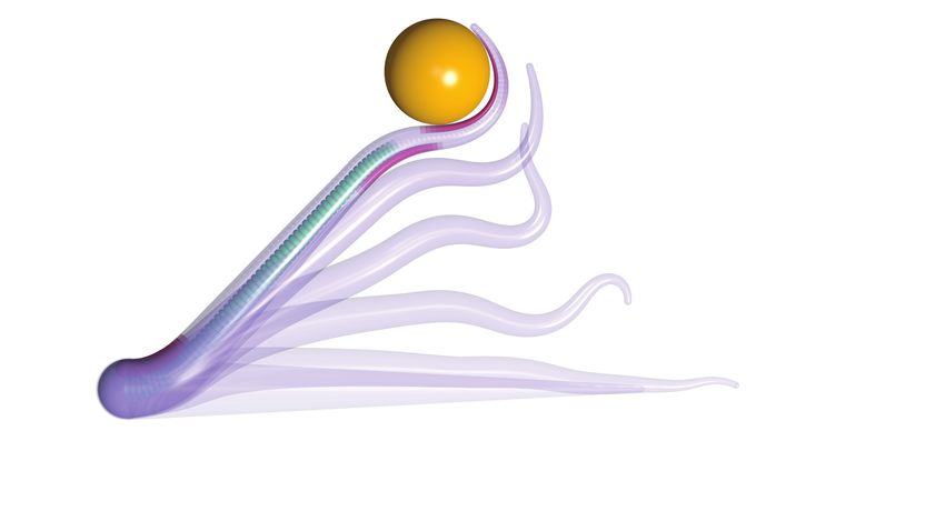
The potential energy of a hyperelastic Cosserat rod model is problems to be solved by our model arm. In this work, the
given by1 control objective is to design stabilizing distributed muscle
Z L0 activations so that – (i) the tip reaches a target point, and (ii)
Ve = W e (w) ds (2) the arm wraps around an object to grasp it.
0
III. C ONTROL - ORIENTED MODELING OF MUSCLES
where W e (w) = W e (ν1 , ν2 , κ) is referred to as the elastic
stored energy function. The simplest model of the stored In this section, the control-oriented modeling of internal
energy function is of the quadratic form muscles is presented. The main results of this section are
given in Proposition 3.1 and Corollary 3.1. A reader more
1
We = EA(ν1 − ν1◦ )2 + GA(ν2 − ν2◦ )2 + EI(κ − κ◦ )2
interested in the control problem may skip ahead to Sec. III-
2 E which is followed by Sec. IV on control methodology.
where E and G are the material Young’s and shear moduli,
and ν1◦ , ν2◦ , κ◦ are the intrinsic strains that determine the A. Muscle geometry
rod’s shape at rest. If ν1◦ ≡ 1, ν2◦ ≡ 0, κ◦ ≡ 0, then the rest Since we consider planar movement of the arm, the
configuration is a straight rod of length L0 . following muscles are most relevant (see Fig. 1c)
Thus, the overall dynamic model is expressed as a Hamil- 1) The top longitudinal muscle denoted as LMt ,
tonian control system with damping: 2) The bottom longitudinal muscle denoted as LMb ,
3) The transverse muscles in the middle denoted as TM.
dq δT
= For a generic muscle m ∈ {LMt , LMb , TM}, the vector
dt δp
dp δV e X (3) rm = r1m a + r2m b
=− − γM −1 p + Gm (q)um
dt δq m specifies its position with respect to the centerline, as de-
m m
where u = u (s, t) ∈ [0, 1] is the muscle activation and 2 picted in Fig. 1c. For these three muscle groups, coordinates
serves as the control input for our purposes. The operators (r1m , r2m ) are reported in Table I.
Gm model how a (internal) muscle actuation um translates to B. Forces from muscle actuation
resultant (external) forces and couples that move the Cosserat
When activated, a muscle provides an internal distributed
rod. The modeling of Gm is the subject of the next section.
contraction force
The linear damping term models the inherent viscoelasticity
in the arm [20] where γ > 0 is a damping coefficient. nm = nm m
1 a + n2 b
Model (3) is accompanied by suitable initial and boundary
conditions. and because of their (off centerline) geometric arrangement,
the two longitudinal muscles also provide a couple
Remark 1: For a given W e , the internal elastic forces and
couples are given by the stress-strain relationship mm = (rm × nm ) · (e1 × e2 ) = r1m nm m m
2 − r2 n1
∂W e ∂W e where ‘·’ and ‘×’ denote the usual vector dot and cross
ni = , i = 1, 2, m = product, respectively. This yields the following model for
∂νi ∂κ
a single muscle:
where n1 , n2 are the components of the internal force (n) m
in the material frame, i.e. n = n1 a + n2 b, and m is the cos θ − sin θ n1
∂
internal couple. Specifically, the conservative forces on the Gm (q)um = s sin θ cos θ nm
2
(4)
m m m
righthand-side of (3) are as follows [14]: ∂s m + ν1 n2 − ν2 n1
It remains to prescribe a model for the contraction force nm
e cos θ − sin θ n1
δV ∂
− = s sin θ cos θ n2 as a function of the activation um . This is the subject of the
δq following subsections.
∂s m + ν1 n2 − ν2 n1
The quadratic model of the stored energy means that C. Hill’s lumped model of a muscle
the stress-strain relationship is linear. For this reason, the In the Hill’s muscle model [16]–[18], [24], the tension
quadratic model of the stored energy function is referred to produced by muscular activation is modeled using three par-
as linear elasticity. However, elastic characteristics of soft allel lumped elements (Fig. 2): an active contractile element,
tissue can be nonlinear [23]. a passive spring element, and a damping element. When
Control objective: Octopus arms are capable of a variety of a muscle is activated (i.e., um > 0), the active contractile
manipulation tasks [5]. Inspired by this, we set some control element produces a tension force which scales linearly with
activation um ∈ [0, 1], and is described through a force-
1 Here the superscript e stands for elastic potential energy length relationship fl (·), such as the one depicted in Fig. 2.
2 Physically, the control um (s, t) is related to the neuronal stimulation, Maximum forces are produced when the muscle is in its rest
such as the firing frequency of the motor neuron innervating the muscle
fiber at s at time t. The bound on um is a manifestation of maximum firing length configuration, and decreases as the muscle contracts
frequency of a motor neuron. or elongates. The bio-physics of this force-length relationship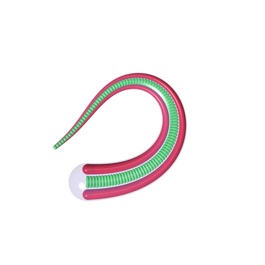
±φLM b. (The sign is positive for the top LM and negative for
                                                                   the bottom LM.) Taking the spatial derivative of the muscle
                                                                   position r + rLM , the local stretch strain is obtained as
                                                                                        ν LM = ν1 ∓ φLM κ
                                                                   When a longitudinal muscle is activated, it generates the
                                                                   contraction force nLM along the longitudinal direction a and
                                                                   also produces the couple mLM . The expressions for these are
                                                                   obtained as
                                                                              nLM = nLM a,        mLM = ∓φLM nLM
Fig. 2: Hill’s muscle model: The three parallel elements are       where nLM is defined using (5) with m = LM and ν m
shown in the inset. The force-length relationship of the active    given by ν LM . The couple mLM bends the arm locally which
contractile element is shown on the right.                         is believed to be one of the most important functionalities
                                                                   of the longitudinal muscle. By symmetry, the parameters Am
is explained by the sliding filament theory of individual          and nmmax are considered to be the same for both the LMt and
muscle fibres [17], [24]. The passive spring element accounts      LMb .
for the elasticity of the muscle. There are also dissipative
                                                                   Transverse muscles: When a transverse muscle (TM) con-
effects which are accounted for through so-called force-
                                                                   tracts, it causes the cross sectional area to shrink. Owing to
velocity relationship of the muscles. The following notation
                                                                   the constancy of volume (tissue incompressibility), the arm
is adopted to model the force-length relationship.
                                                                   extends. Such a behavior is modeled as follows:
   Definition 1: Let fl : R+ → R+ denote the force-
length
Rz      relationship. Define also Fl : R+ → R+ , Fl (z) :=                        nTM = − nTM a,        mTM = 0
   f (z) dz, i.e. Fl0 (z) = fl (z), where the prime indicates
 0 l                                                               where the couple is zero because the transverse muscles
the derivative with respect to the argument.
                                                                   surround the axial nerve cord, i.e. rTM = 0. To capture the
   Remark 2: We note here that a particular form of the            physics of inverse relationship between the stretch strain of
function fl (·) is not instrumental to the muscle modeling         the arm and that of the transverse muscles, we model the
and control design, and can be replaced by an experimentally       local stretch strain of transverse muscle as
obtained relationship. The specific form of the force-length
                                                                                                ν1◦         ν1
relationship used here is a 3rd degree polynomial fit to                               ν TM =   ν1    ≈2−   ν1◦
experimental data for squid tentacle muscles [25, Fig. 6].
                                                                   For simplicity, we adopt a linear approximation at ν1 = ν1◦ .
The formula appears in Sec. V.
                                                                      These complete the modeling of the longitudinal and
   Remark 3: Similar to [19], [26], in this paper the other        transverse muscles. The formulae for muscle stretch strain,
two elements – passive spring and the dashpot – are not            forces, and couples are reported in Table I.
explicitly modeled. The effects of these elements are consid-
ered to be assimilated in the inherent viscoelasticity of the      E. Muscle energy function
Cosserat rod, i.e. the gradient of V e term and the damping           The main result of this section is to obtain the muscle
term in (3).                                                       forces and couples (nm , mm ) from a stored energy func-
                                                                   tion. The proof of the following proposition appears in
D. Muscle model adaptation to Cosserat rod formalism
                                                                   Appendix I.
   Here we adapt the Hill’s active force model as follows.
For a generic muscle m, the magnitude of the active internal         Proposition 3.1: Suppose um = um (s, t) is a given acti-
force is                                                           vation of a generic muscle m. Then there exists a function
                                                                   W m = W m (ν1 , ν2 , κ) such that the internal muscle forces
            |nm | = nm    m        m     m
                     max A (s)fl (ν (s))u (s, t)            (5)    and torques are given by
where Am is the arm cross sectional area occupied by the                             ∂W m                         ∂W m
                                                                           nm
                                                                            i =u
                                                                                 m
                                                                                          , i = 1, 2,   mm = um               (6)
muscle, nm  max is the maximum producible force per unit                              ∂νi                          ∂κ
area. In the context of this paper, the appropriate ‘length’       The expressions of the function W m for the two longitudinal
is the stretch strain ν m of the muscle. It is a function of the   muscles LMt and LMb , and the one transverse muscle TM
deformation w. In the following, we describe the models –          appear in Table I.
expressions for nm , mm , ν m for the two types of muscles:
                                                                      The total stored energy function for the arm is defined as
Longitudinal muscles: The top and the bottom longitudinal          follows:
muscles (LM) are positioned at a distance φLM (s) away                                                X
from the rod center line. Hence, the position vector of a                      W (w; u) := W e (w) +      um W m (w)
longitudinal muscle is given as r + rLM , where rLM =                                                   m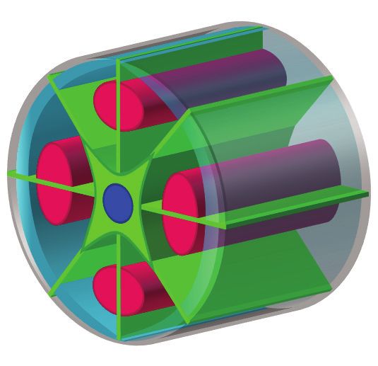
TABLE I: Summarized muscle model
Muscle model notation Parameter values for simulation
m rm νm nm mm Wm off center max stress cross sectional
muscle position muscle strain muscle force muscle couple muscle stored energy distance [kPa] area
LMt φLM b ν1 − φLM κ nLMt a −φLM nLM
t nLM
max A
LM (s)F (ν LMt )
l
2φ(s) A
φLM = nLM
max = 19.89 ALM =
−φLM b ν1 + φLM κ nLMb a φLM nLMb nLM LM (s)F (ν LMb ) 3 9
LMb max A l
ν1 A
TM 0 2− ν1◦
− nTM a 0 nTM
max A
TM (s)F (ν TM )
l φTM = 0 nTM
max = 13.26 ATM =
12
where u = {um }. This results in the potential energy Then the control law (9) renders the equilibrium (qα , 0) of
Z L0 X (3) (locally) asymptotically stable.
V(u) := W (w; u) ds = V e + V m (um ) A sketch of the proof of Proposition 4.1 is given as fol-
0 m (7) lows. According to Corollary 3.1, application of the control
Z L0
where V m (um ) := um (s, t)W m (w(s, t)) ds law (9) makes the closed loop system a damped Hamiltonian
0 system with closed loop Hamiltonian Htotal = T + V(α).
Using this notation, we obtain the following corollary: The local convexity assumption of W (w; α) lets us take the
closed loop Hamiltonian Htotal as a Lyapunov functional.
Corollary 3.1: Suppose um = um (s, t) is a given activa- Then along a solution trajectory of (3) with controls (9),
tion of the muscle m. Then the muscle-actuated arm is a we have
Hamiltonian control system with the Hamiltonian
dHtotal 2
Htotal = T + V e +
X
V m (um ) = −γ M −1 p ≤0
dt
m
where the norm is taken in the L2 sense. We thus have
In particular, the muscle forces in (3) are given by
that the total energy of the system is non-increasing. Fi-
δV m nally, an application of the LaSalle’s theorem guarantees
Gm (q)um = −
δq local
n asymptotictotal stability
o to the largest invariant subset
We omit the proof of Corollary 3.1 due to lack of space. of (q, p) dHdt = 0 , which is indeed the equilibrium
The proof proceeds in the same way as showing the passive point (qα , 0). Note that a complete proof of Proposition 4.1
elasticity term in (3) is the (negative) gradient of the arm’s involves rigorous arguments of a LaSalle’s principle in the
intrinsic potential energy function [14]. infinite dimensional setting, which is beyond the scope of
How to design the muscle activation um to solve a control this paper.
problem is the main question addressed in the following Remark 4: In general, for underactuated Hamiltonian con-
section on energy shaping. trol systems, the energy shaping methodology requires solv-
ing a PDE called the matching condition [10]–[12]. Our for-
IV. E NERGY SHAPING CONTROL DESIGN
mulation of the muscle model enables us to write the control
A. Energy shaping control law terms Gm um as Hamiltonian vector fields (Corollary 3.1).
In order to obtain and analyze the equilibrium (stationary Consequently, the constant control law (9) is a solution to
point of the potential energy), the following definition is the resulting matching condition for this problem. This line
useful: of thinking is elucidated in [27].
Definition 2: Suppose um = αm (s) is a given time- Thus it remains to design the static controls α that
independent activation of the muscle m and α = {αm }. Then shape the potential energy. This is the subject of the next
the gradient and the Hessian of W are denoted as subsection.
∂W (w; α) ∂P ∂ 2 W (w; α)
P (w; α) := , Q(w; α) := = (8) B. Design of potential energy: The static problem
∂w ∂w ∂w2
The following proposition prescribes an energy shaping The problem of designing the muscle activation α is posed
control law. as an optimization problem:
Proposition 4.1: Consider the control system (3) with a
minimize [muscle related cost] + [task related cost]
constant muscle control α∈[admissible set]
um (s, t) ≡ αm (s), t≥0 (9) subject to equilibrium constraints (of the rod)
and task related constraints
Suppose the potential energy functional V(α) has a minimum
at the deformations wα with associated configuration qα . This optimization problem is an example of a bilevel opti-
Additionally, let the muscle parameters be such that the mization problem, also referred to as structural optimization
Hessian Q(w; α) is locally positive definite at w = wα . problem in literature [28], [29].1) Lower level optimization – obtain the equilibrium Algorithm 1 Solving the bilevel optimization problem
constraints: This is an example of a forward problem. For a Input: Task (reaching, grasping)
given (fixed) α, obtain the equilibrium (or a static) configura- Output: Optimal activations ᾱ = (ᾱLMt , ᾱLMb , ᾱTM )
tion of the rod. The equilibrium is obtained by calculating the 1: Initialize: activations α(0) , states at base: q(0) = 0
2: for k = 0 to MaxIter do
minimum of the total potential energy V(α) [29] as follows:
(k) lower
Z L0 3: Solve (13) to obtain wα
level
minimize V = W (w(s); α) ds 4: Update forward (1)
higher
w(·) 0 (10) 5: Update backward (A-2), (A-1)
level
(k+1) (k) ∂ Ĥ
subject to (1), with boundary conditions 6: Update activations: α = α + η ∂α
7: Limit activations α(k) within [0, 1]
where we recall (1) is the kinematic constraint of the rod.
8: end for
The necessary conditions for optimality are obtained from
9: Output the final activations as ᾱ
the Pontryagin’s Maximum Principle (PMP) as follows: De-
note the costate to q(s) as λ(s) = (λ1 (s), λ2 (s), λ3 (s))| ∈
the activation α that solves the task. For this purpose, we
R3 . Then the control Hamiltonianfor this problem is propose the following optimization problem:
H(q, λ, w) = λ| g(q, w) − W (w; α) 1
Z L0 X 2
minimize J(α) = (αm (s)) ds
m
α(·), α (s)∈[0,1] 2 0
The costate λ evolves according to Hamilton’s equation m
Z L0
+ µgrasp (s)Φgrasp (q(s)) ds + µtip Φtip (q(L0 ), q ∗ ) (14)
0
0
∂H 0
subject to ∂s q = g(q, wα ), q(0) = 0, q(L0 ) free;
∂s λ = − = (11)
∂q {−ν1 (−λ1 sin θ + λ2 cos θ) and Ψj (q) ≤ 0, j = 1, 2, ..., Nobs
ν2 (λ1 cos θ + λ2 sin θ)}
The significance of the terms is as follows:
Pointwise maximization of the control Hamiltonian leads to
1) The quadratic term is used to model the control cost of
the requirement that
using muscles.
|
2) The function Φtip is used to model the control task for
∂g
λ − P (w; α) = 0 (12) the tip, e.g., to reach a given point in space.
∂w
3) The running cost Φgrasp is used to model the control task
In general settings, (1), (11) and (12) together with the for the whole arm, e.g., for the arm to wrap around an
appropriate boundary conditions (see e.g. [4], [30]) represent object.
the equilibrium constraint obtained from the lower level op- 4) Equation (14) is used to model the obstacles in the
timization problem. Considerable simplification arises when environment as state constraints of the form Ψ(q) ≤ 0.
the boundary conditions are of the fixed-free type. This case
The formulae for these functions and parameters (e.g.
is of particular interest for the CyberOctopus control problem
µgrasp , µtip ) are task-specific and appear in Sec. V. The
where the arm is attached to the head, i.e. the base is fixed
higher level optimization problem (14) is an optimal control
(and without loss of generality can be taken as 0). The tip is
problem for the kinematics (1) with α as controls, whose
free since there is no externally imposed boundary condition
necessary conditions for optimality are obtained by PMP and
at the tip. The result is described in the following proposition:
are summarized in Appendix II.
Proposition 4.2: Consider the optimization problem (10)
with the boundary conditions q(0) = 0 and q(L0 ) 3) Algorithms: Given any task, we solve the bilevel opti-
free. Then any minimizer, denoted by wα (s) = mization problem in an iterative manner. In each iteration,
(ν1,α (s), ν2,α (s), κα (s)), must satisfy for all s ∈ [0, L0 ] we first solve the lower level problem, i.e. solve the nonlinear
EA(ν1,α (s) − 1)
P m
n1 (s, wα (s); αm )
equations (13) for wα pointwise in s. We utilize the fsolve
P (wα ; α) = GAν2,α (s) + P 0 =0 routine in the scipy package for this purpose. The higher level
EIκα (s) mm (s, wα (s); αm ) problem (14) is then solved by using a forward-backward
(13) algorithm to obtain the optimal α (see also Sec. III-C in
Proof: Indeed, when q(L0 ) is free, the PMP equa- [4]). In Algorithm 1, we give a brief pseudo code of the
tions need to be augmented by the transversality condition algorithm. Finally according to Proposition 4.1 the energy
λ(L0 ) = 0 which, by the virtue of costate evolution equa- shaping controls are simply the optimal α.
tions (11), leads to λ ≡ 0 for all s. Equation (12) then A more comprehensive discussion on algorithms for solv-
simplifies to (13) at w = wα . ing this problem appears in our prior work [4].
In summary, equation (13) is the equilibrium constraint V. N UMERICAL SIMULATION
from solving the forward problem (for a given α). In this section, a numerical environment is used to demon-
2) Upper level optimization – obtain the optimal static strate the abilities of a soft octopus arm under our control
actuation: This is an example of an inverse problem. For algorithm. Two experiments are shown to mimic the behav-
a given set of control-specific tasks and constraints, obtain iors of reaching and grasping motion of an octopus arm.REACHING STATIC TARGETS GRASPING A STATIC TARGET
(a) (b) (c) (d)
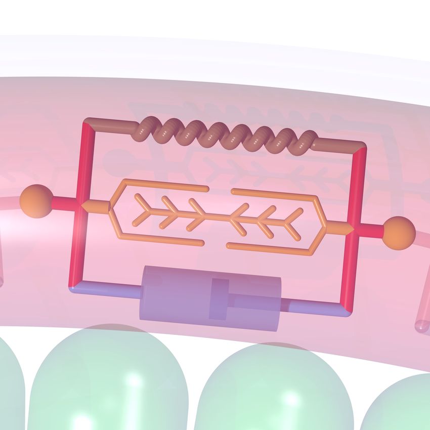
Fig. 3: Reaching task (a-b). The arm is tasked to reach three different locations one after the other, mimicking the octopus’
fetching motions. (a) Targets are located at (12, 14), (16, 6) and (2, −2) [cm] and are indicated as orange spheres. Optimal
arm configurations are depicted together with muscle activations. The time evolution of the arm is depicted as transparent
purple rods. (b) Dotted lines show the activations at t = 0 [s]; dash-dot lines show the activations at t = 1.5 [s]; and solid
lines show the activations at t = 3.5 [s]. Grasping task (c-d). The arm is tasked to wrap around a static sphere (the big
orange sphere) of radius 2 [cm] centered at (12, 12) [cm]. (d) The solid line shows the activations at t = 2.5 [s].
A. Simulation setup TABLE II: Parameters
The explicit dynamic equations of motion (3) of a pla- Parameter Description Value
nar Cosserat rod [14] are discretized into Nd connected L0 rest arm length [cm] 20
cylindrical segments and solved numerically by using our φbase base radius [cm] 1.2
open-source, dynamic, three-dimensional simulation frame- φtip tip radius [cm] 0.12
E Young’s modulus [kPa] 10
work Elastica [20]–[22]. The radius profile of the tapered G Shear modulus [kPa] 40/9
geometry of an octopus arm is modeled as ρ density [kg/m3 ] 1050
γ dissipation [kg/s] 0.02
φ(s) = φtip s + φbase (L0 − s) Nd discrete number of elements 100
∆t discrete time-step [s] 10−5
with the cross sectional area and the second moment of area η learning rate 10−8
2
as A = πφ2 and I = A 4π . We take the rest configuration
of the rod to be straight of length L0 , i.e. (ν1◦ , ν2◦ , κ◦ ) ≡ where φobj and robj denote the radius and center position of
(1, 0, 0). The biologically realistic parameter values in this the object, respectively. In addition, since we want the arm
work are listed in Table I and II and also in reference [4]. to grasp the target sphere, the running cost Φgrasp and the
The following force length curve fl (·) for the Hill’s muscle weight function µgrasp in (14) are designed so that the arm
model is used: can get as close to the boundary as possible:
3.06z 3 − 13.64z 2 + 18.01z − 6.44, if 0.6 ≤ z ≤ 1.6
n
fl (z) = 0, Φgrasp (q(s)) = dist(Ω, r(s)), µgrasp (s) = 105 χ[0.4L0 ,L0 ] (s)
else
This model is fitted from experimental data [25, Fig. 6]. where Ω denotes the boundary of the object (here just a
circle), dist(·, ·) calculates the distance between the boundary
B. Experiments and the point r(s), and χ[s1 ,s2 ] (·) denotes the character-
1) Reaching multiple static targets: The first experiment istic function of [s1 , s2 ]. Such a design together with the
consists reaching multiple targets one by one to mimic the inequality constraint cause the distal portion of the arm,
behavior of a real octopus. For any target, the tip cost starting from s = 0.4L0 , to grasp the target sphere without
function Φtip in (14) is set as penetrating it. The value of µtip is 0 in this case. Fig. 3(c-d)
1 ∗ 2
shows the simulation results where the arm grasps the sphere
Φtip (q(L0 ), r∗ ) = |r − r(L0 )| under its muscle actuation model.
2
where r∗ is the target position. The cost does not depend on VI. C ONCLUSION AND FUTURE WORK
the tip angle θ(L0 ) as we are not concerned about the tip
pose. The weight function µgrasp is chosen to be zero and In this paper, a flexible octopus arm is represented as a
regularization parameter µtip is set as 105 . Simulation results planar Cosserat rod and its muscle mechanisms are modeled
are shown in Fig. 3(a-b). as distributed internal force/couple functions with the muscle
2) Grasping an object: In the second experiment, the activations as the control inputs. The rod is viewed as an
octopus arm is tasked to grasp a target sphere. This behavior underactuated Hamiltonian control system, for which an
is commonly seen when an octopus is trying to reach for a energy shaping control method is sought to solve various
bottle, a shell or a crab. To find the desired static configura- manipulation objectives, e.g. reaching and grasping. We have
tion via (14), the object is treated as both an obstacle and a shown that the total energy of the closed loop system can
target so that the arm cannot penetrate it but can wrap around be expressed by augmenting the inherent elastic energy of
it. The inequality constraint model of it is: the rod with muscle stored energy functions. As a result,
2 constant muscle controls stabilize the arm. A bilevel opti-
Ψ(q(s)) = φobj + φ(s) − |robj − r(s)|2 mization problem is then constructed and solved numericallyto obtain desired muscle controls for a given task. Numerical [23] F. Tramacere et al., “Structure and mechanical properties of octopus
experiments demonstrate the efficacy of this scheme. As vulgaris suckers,” Journal of The Royal Society Interface, vol. 11,
no. 91, p. 20130816, 2014.
a direct extension, a more sophisticated muscle actuation [24] Y.-c. Fung, Biomechanics: mechanical properties of living tissues.
model and the corresponding control method can be applied Springer Science & Business Media, 1996.
to the general 3D case. Another direction of future work [25] W. M. Kier and N. A. Curtin, “Fast muscle in squid (loligo pealei):
contractile properties of a specialized muscle fibre type,” Journal of
is to develop an octopus-inspired neuromuscular control Experimental Biology, vol. 205, no. 13, pp. 1907–1916, 2002.
where muscle activation is controlled by underlying neuronal [26] Ö. Ekeberg, “A combined neuronal and mechanical model of fish
activity. The problem of sensorimotor control can also be swimming,” Biological cybernetics, vol. 69, no. 5, pp. 363–374, 1993.
[27] B. Maschke et al., “Energy-based lyapunov functions for forced hamil-
considered where only a part of the state is available to the tonian systems with dissipation,” IEEE Transactions on automatic
controller through internal distributed sensors. control, vol. 45, no. 8, pp. 1498–1502, 2000.
[28] B. Colson et al., “An overview of bilevel optimization,” Annals of
R EFERENCES operations research, vol. 153, no. 1, pp. 235–256, 2007.
[29] J. Outrata et al., Nonsmooth approach to optimization problems with
[1] D. Rus and M. T. Tolley, “Design, fabrication and control of soft equilibrium constraints: theory, applications and numerical results.
robots,” Nature, vol. 521, no. 7553, pp. 467–475, 2015. Springer Science & Business Media, 2013, vol. 28.
[2] G. Singh and G. Krishnan, “A constrained maximization formulation to [30] T. Bretl and Z. McCarthy, “Quasi-static manipulation of a Kirchhoff
analyze deformation of fiber reinforced elastomeric actuators,” Smart elastic rod based on a geometric analysis of equilibrium configura-
Materials and Structures, vol. 26, no. 6, p. 065024, 2017. tions,” The International Journal of Robotics Research, vol. 33, no. 1,
[3] C. Della Santina et al., “Dynamic control of soft robots interacting pp. 48–68, 2014.
with the environment,” in 2018 IEEE International Conference on
Soft Robotics (RoboSoft). IEEE, 2018, pp. 46–53. A PPENDIX I
[4] H.-S. Chang et al., “Energy shaping control of a cyberoctopus soft
arm,” in 2020 59th IEEE Conference on Decision and Control (CDC). P ROOF OF P ROPOSITION 3.1
IEEE, 2020, pp. 3913–3920. Proof: Indeed, for the top longitudinal muscle LMt ,
[5] G. Levy et al., “Motor control in soft-bodied animals: the octopus,”
in The Oxford Handbook of Invertebrate Neurobiology, 2017. define W LMt := ALM nLM max Fl (ν1 − φ
LM
κ). Then it readily
[6] W. M. Kier and M. P. Stella, “The arrangement and function of octopus follows by using the definition of the function Fl that
arm musculature and connective tissue,” Journal of Morphology, vol.
268, no. 10, pp. 831–843, 2007. ∂W LMt
nLM
1
t
= nLMt = uLMt
[7] W. M. Kier, “The musculature of coleoid cephalopod arms and ∂ν1
tentacles,” Frontiers in cell and developmental biology, vol. 4, p. 10,
∂W LMt
2016. mLMt = −φLM nLMt = uLMt
[8] N. Feinstein et al., “Functional morphology of the neuromuscular ∂κ
system of the octopus vulgaris arm,” Vie et milieu (1980), vol. 61, LMt
no. 4, pp. 219–229, 2011. Additionally, it is obvious that nLM
2
t
= ∂W
∂ν2 = 0. Similar
[9] N. Nesher et al., “From synaptic input to muscle contraction: arm arguments follow for other two muscles.
muscle cells of octopus vulgaris show unique neuromuscular junction
and excitation–contraction coupling properties,” Proceedings of the A PPENDIX II
Royal Society B, vol. 286, no. 1909, p. 20191278, 2019.
[10] R. Ortega et al., “Stabilization of a class of underactuated mechanical
PMP CONDITIONS FOR PROBLEM (14)
systems via interconnection and damping assignment,” IEEE transac- Here we only express the key PMP conditions. For more
tions on automatic control, vol. 47, no. 8, pp. 1218–1233, 2002.
[11] G. Blankenstein et al., “The matching conditions of controlled la-
explanations, please refer to [4]. For the constrained opti-
grangians and ida-passivity based control,” International Journal of mization problem (14), the original state q is augmented to
Control, vol. 75, no. 9, pp. 645–665, 2002. include Nobj additional states q̂j which has the following
[12] A. M. Bloch et al., “Controlled lagrangians and the stabilization of
mechanical systems. i. the first matching theorem,” IEEE Transactions
evolution:
on automatic control, vol. 45, no. 12, pp. 2253–2270, 2000. ∂s q̂j = cj (q) = max(Ψj (q), 0), q̂j (0) = 0, j = 1, ..., Nobs
[13] D. Auckly et al., “Control of nonlinear underactuated systems,”
Communications on Pure and Applied Mathematics, vol. 53, no. 3, and the terminal cost function is also modified as follows
pp. 354–369, 2000. X
[14] S. S. Antman, Nonlinear Problems of Elasticity. Springer, 1995. Φ̂(q(L0 )) = µtip Φtip (q(L0 ), q ∗ ) + ξj q̂j (L0 )
[15] T. J. Healey and P. G. Mehta, “Straightforward computation of spatial
equilibria of geometrically exact cosserat rods,” International Journal where ξj > 0 are the weights for the augmented states
of Bifurcation and Chaos, vol. 15, no. 3, pp. 949–965, 2005.
[16] A. V. Hill, “The heat of shortening and the dynamic constants of q̂j (L0 ). Denoting the costate of q as λ̂, the modified control
muscle,” Proceedings of the Royal Society of London. Series B- Hamiltonian Ĥ is written as
Biological Sciences, vol. 126, no. 843, pp. 136–195, 1938. 1 2
[17] D. A. Winter, Biomechanics and motor control of human movement. Ĥ(s, q, λ̂, α) = λ̂| g(q, wα ) − |α| − µgrasp (s)Φgrasp (q)
John Wiley & Sons, 2009. 2
[18] M. Audu and D. Davy, “The influence of muscle model complexity
in musculoskeletal motion modeling,” 1985. The costate λ̂ must satisfy the Hamilton’s equation
[19] Y. Yekutieli et al., “Dynamic model of the octopus arm. i. biomechan-
ics of the octopus reaching movement,” Journal of neurophysiology,
∂ Ĥ X ∂cj
∂s λ̂ = − + ξj (A-1)
vol. 94, no. 2, pp. 1443–1458, 2005. ∂q ∂q
[20] M. Gazzola et al., “Forward and inverse problems in the mechanics of
soft filaments,” Royal Society Open Science, vol. 5, no. 6, p. 171628, with the accompanied transversality condition
2018. ∂Φtip
[21] X. Zhang et al., “Modeling and simulation of complex dynamic λ̂(L0 ) = −µtip (q(L0 ), q ∗ ) (A-2)
musculoskeletal architectures,” Nature Communications, vol. 10, no. 1, ∂q
pp. 1–12, 2019.
[22] N. Naughton et al., “Elastica: A compliant mechanics environment for and the optimal α should maximize the Hamiltonian Ĥ
soft robotic control,” IEEE Robotics and Automation Letters, 2021. pointwise in [0, L0 ].You can also read