Predictive Runtime Monitoring for Mobile Robots using Logic-Based Bayesian Intent Inference
←
→
Page content transcription
If your browser does not render page correctly, please read the page content below
Predictive Runtime Monitoring for Mobile Robots using Logic-Based
                          Bayesian Intent Inference
                                          Hansol Yoon and Sriram Sankaranarayanan .

   Abstract— We propose a predictive runtime monitoring                                      Mobile Robot
framework that forecasts the distribution of future positions                                                                   H1
of mobile robots in order to detect and avoid impending
                                                                                                                      H2
property violations such as collisions with obstacles or other
agents. Our approach uses a restricted class of temporal logic
formulas to represent the likely intentions of the agents along                                       H3
with a combination of temporal logic-based optimal cost path
planning and Bayesian inference to compute the probability of
these intents given the current trajectory of the robot. First,
we construct a large but finite hypothesis space of possible
intents represented as temporal logic formulas whose atomic                   Env. Info
                                                                                                                                             Observation
propositions are derived from a detailed map of the robot’s                               Hypothesis Generation                 Evaluation
workspace. Next, our approach uses real-time observations of                                                       Hypotheses
                                                                                     H1: Avoid mountain, go to A      Set        H1: 45%
the robot’s position to update a distribution over temporal logic                    H2: Go to B                                 H2: 35%      Trajectory
formulae that represent its likely intent. This is performed                         H3: Go to C                                 H3: 20%      Prediction
by using a combination of optimal cost path planning and
a Boltzmann noisy rationality model. In this manner, we
construct a Bayesian approach to evaluating the posterior                Fig. 1. The proposed Bayesian intent inference approach first generates
                                                                         a hypotheses set (H1-H3) and uses the robot’s recent positions to update
probability of various hypotheses given the observed states and
                                                                         the probability of various hypothesized intents (H1-H3). Finally, we can
actions of the robot. Finally, we predict the future position            predict likely future positions of the robot using the inferred distribution
of the robot by drawing posterior predictive samples using a             over possible intents.
Monte-Carlo method. We evaluate our framework using two
different trajectory datasets that contain multiple scenarios
implementing various tasks. The results show that our method
can predict future positions with precisely and efficiently, so          performing. In this paper, we term this as the robot’s (cur-
that the computation time for generating a prediction is a tiny          rent/short term) intent. This approach assumes that the robot
fraction of the overall time horizon.                                    has a high-level mission or intent. Furthermore, the robot is
                     I. INTRODUCTION                                     assumed to choose an “efficient” plan for implementing the
                                                                         mission. The efficient path can be either the shortest path or
   Detecting and preventing imminent property violations is              the almost shortest path. In many scenarios, this assumption
an important problem for the safe operation of autonomous                is reasonable since operators want robots to implement more
robots in highly dynamic environments. Such violations                   missions with limited resources. Therefore, if a robot does
include collisions between multiple robots, failure to respond           not choose an efficient strategy for completing a task, we
to events or robots entering restricted areas. Detecting such            can deduce that either the robot is not rational or that our
violations at design time is often impractical: behaviors are            current model of the robot’s goals are incorrect [7]–[13].
dependent on possible environmental conditions. The space                   In this paper, we use the robot’s intent information for
of possible behaviors is too large, or may not be com-                   predictive runtime monitoring. Our assumption is that, if a
pletely known to the designers. Thus, runtime monitoring                 robot has a high-level mission, we are able to (1) not only
approaches have recently gained popularity. However, these               infer the mission by observing its behavior (2) but also use
approaches require a model of the robot’s motion to predict              the information to predict future positions. Therefore, the
its future position. Recent approaches have employed such                ability to find the intent is key in our work.
models to detect the possible positions that a robot can                    To that end, we use temporal logic formulas to represent
reach in the near future using physics-based dynamic models              the intent. Temporal logics have been quite popular for
and reachability analysis [1]–[4]. Similarly, a pattern-based            specifying missions in a precise manner and generating
approach predicts future positions based on historical data              efficient plans for carrying them out [14]–[20]. Temporal
and predicts likely future positions [5] (Cf. [6] for a survey           logics have been demonstrated as suitable reprentations of
of trajectory prediction for dynamic agents).                            complex real-world missions such as surveillance and pack-
   However, forecasting future moves by extrapolating the                age delivery [18], [21]–[23]. We identify a subset of temporal
past trajectories is often likely to fail unless we also have a          logic formulas corresponding to the safety and guarantee
specification of the task (or current subtask) that a robot is           formulas in the Manna-Pnueli hierarchy of temporal logic
  Department of Computer Science, University of Colorado Boulder, USA,   formulas [24]. Such formulas can be satisfied or violated by
{firstname.lastname}@colorado.edu                                        a finite prefix of an infinite sequence of actions and thus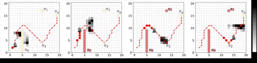
quite suitable as representations of “near-term”/“immediate”       wherein C is a finite set of cells, R ⊆ C ×C is the transition
intents suitable for finite time horizon predictions of the        relation that represents all allowable moves from one cell
robot’s position. The Bayesian intent inference framework          to the next by the robot, Π is a set of boolean atomic
then generates a finite set of possible intents using given        propositions, L : C → 2Π is a labeling function that associates
patterns of temporal logic formulas and places a prior             each cell c ∈ C with a set of atomic propositions L(c), and
distribution on these formulas to represent the probability        ω : R → R≥0 maps each edge in R to a non-negative weight.
that a given formula represents the robot’s intent. Next, we          Therefore, the position of a robot at time t can be defined
use a model of “noisy rationality” to provide a probability        as a cell xt ∈ C. Atomic propositions label attributes/features
that a robot takes a given action in the workspace given           such as airport, fire, mountain, and so on (see Fig. 1). A path
its true intent. This model compares the cost of the action        in T is an infinite sequence of cells p = c0 c1 c2 · · · such that
and the most efficient path from the resulting state to the        ci ∈ C and (ci , ci+1 ) ∈ R for each i ∈ N.
overall goal of the intent against other possible actions. We
                                                                        a) Linear Temporal Logic: In this paper, we assume
use temporal logic planning techniques based on converting
                                                                   that a robot has a high-level mission to implement before
formulas to automata and solving shortest path problems to
                                                                   going to a goal location. For example, “H1 : Visit π1 , π2 , and
compute these costs.
                                                                   π3 in some order”, or “H2 : Visit π3 while avoiding π5 ”. To
   Temporal logic specification inference from observation
                                                                   formally express such requirements, we use linear temporal
data have been studied widely in the recent past [25]–[28].
                                                                   logic (LTL) whose grammar is defined as follows:
The main difference from our work is that they assume the
entire trajectory is available at once, whereas we use the parts
of the trajectory. Furthermore, our approach uses intents as             ϕ ::= true | false | π ∈ Π | ¬ϕ | ϕ ∧ ϕ | #ϕ | ϕ U φ .
a means to perform predictions of future positions.
   We evaluate our framework on two datasets: a probabilistic      In addition, two temporal operators, eventually (♦ϕ :
roadmap simulation dataset, wherein we use the popular             true U ϕ) and globally (ϕ : ¬♦¬ϕ) can be derived. The
PRM planning technique to generate motion plans for some           formula ϕ is satisfied if ϕ holds for all time and ♦ϕ is
tasks while using our intent inference technique to predict the    satisfied if eventually at some point in time ϕ is satisfied.
intents and future positions without knowledge of the overall      We refer the reader to standard texts for a detailed description
mission plan. A second data set consists of trajectories of        of temporal logic and its applications [30], [31]. Using LTL,
humans inside a room, called TḦOR [29]: here we are               we can express the mission H1 : ♦π1 ∧ ♦π2 ∧ ♦π3 and
provided noisy position measurements with unknown intents.         H2 : ♦π3 ∧ ¬π5 . Using LTL is beneficial because it is ca-
Thus, both datasets include a moving agent implementing            pable of describing complex missions clearly although some
various subtasks on the way to a goal, which is unknown to         fundamental properties like safety (¬ϕ) and reachability
our monitor. The results show that our method can predict          (♦ϕ) are mostly used for robot missions in many scenarios,
future positions with high accuracy, and all computations can      and because it enables us to use temporal logic motion
be implemented in real-time.                                       planning [14]–[20].
   The contributions of this paper are as follows:
                                                                          b) Assumptions: We assume full knowledge of the
  1) We introduce a Bayesian intent inference framework
                                                                   transition system T is available at any time. Also, if the
      leveraging an intent information of a robot. The frame-
                                                                   map is updated in the case of dynamic scenarios, the new
      work computes the probability distribution of all possi-
                                                                   information is assumed to be available immediately. On the
      ble intents written in LTL.
                                                                   other hand, the robot’s mission is assumed to be unknown
  2) Using the outputs of the framework, we can effectively
                                                                   but expressible as a temporal logic formula involving atomic
      carry out predictive monitoring that can be used in many
                                                                   propositions in the map.
      robotic applications.
  3) All computations can be implemented with sufficient               In this paper, we investigate two problems — intent
      efficiency to enable real-time monitoring.                   inference and predictive monitoring. Fig. 2 shows how these
   To the best of our knowledge, this work is the first attempt    problems relate to each other in our proposed framework.
to use a logic-based Bayesian intent inference for predictive      Intent Inference: Given a transition system T
monitoring.                                                        and the recent history of robot cells at time t,
                                                                   xt , xt−1 , · · · , xt−h , we wish to infer a distribution of likely
               II. P ROBLEM F ORMULATION                           intents{(ϕ1 , p1 ), . . . , (ϕn , pn )}, wherein ϕi is a temporal
   Central to our framework is a “map” of the robot’s              logic formula involving atomic propositions Π, and pi ≥ 0
workspace that is discretized into finitely many cells. Each       is its associated probability with ∑ni=1 pi = 1.
cell is labeled with an atomic proposition that characterizes      Predictive Monitoring: Given a distribution over intents, we
the attributes of the cell. We use the mathematical model of       wish to compute a distribution of future positions xt+k at time
a weighted finite transition system to capture the map (or the     t + k. At time t + 1, our approach receives new robot position
workspace) of the robot.                                           xt+1 , requiring updates to the intents, and the predicted future
   Definition 1 (Weighted Finite Transition System): A             cell. This update needs to be computed in time that is much
weighted finite transition system T is a tuple (C, R, Π, L, ω)     smaller than the overall sampling time.
Hypothesis Generation Hypothesis Evaluation proposition π; q0 is an initial state and F is the set of
Environment accepting state.
Hypotheses Given an infinite sequence of atomic propositions
Transition System Observation xt
π0 , π1 , π2 , . . ., a run of the automaton is an infinite sequence
T
ϕ0 : P0 of states q0 , q1 , q2 , . . ., such that q0 is the initial state and
LTL Specs ϕ1 : P1 Bayesian Inference (qi , πi , qi+1 ) ∈ E for all i ≥ 0. Finally, a run is accepting
Büchi Automata .. P(ϕ0···i |xt ) iff it visits an accepting state q ∈ F infinitely often. It is
A0···i . well-known that every LTL formula can be translated into a
ϕi : Pi Post.
Büchi automaton [30], [31]. The problem of constructing a
Posterior Büchi automaton from a LTL specification has been widely
Update
Product Automata studied [34] with numerous tools such as SPOT [35].
T ⊗ A0···i = P0···i a) Safety/Guarantee Formulas and Automata: In this
Predict positions paper, we focus on a very specific class of safety and guar-
antee formulas, originally introduced by Manna & Pnueli
Fig. 2. Diagram of the Bayesian intent inference framework
as part of a larger classification of all LTL formulas [24].
Briefly, safety formulas can be written using the operator
with negations appearing only in front of atomic proposi-
III. BAYESIAN I NTENT I NFERENCE tions, whereas guarantee formulas are written using the ♦
operator with negations appearing only in front of atomic
We first introduce our Bayesian approach to solve the
propositions.
intent inference problem. The idea of our approach is to
Example 2: Going back to the Example 1, we note that
generate possible intents as our hypotheses and evaluate their
the “avoid regions” pattern is a safety formula, whereas the
probabilities using Bayesian inference (see Fig. 2).
“cover regions” and “temporal sequencing” patterns are guar-
A. Hypothesis Generation antee formulas. Note that the coverage with the safety pattern
Hypothesis generation is achieved using temporal logic is the conjunction of a guarantee sub-formula (involving ♦)
specification patterns that have been explored in previous and a safety sub-formula (involving ).
works (Cf. [16], [18]). Such patterns specify temporal logic Assumption: We will assume that any hypothesis being
formulae with “holes” that can be filled in with atomic considered can be written as
! !
M N
propositions. Each such pattern defines a set of formulas ^ ^
obtained by substituting all possible atomic propositions ¬πs,i ∧ ♦πg, j , (1)
i=1 j=1
of interest for each hole. To avoid potentially vacuous or
inconsistent intents, we may further require that the same wherein A : {πs,1 , . . . , πs,M } is disjoint from B :
atomic proposition not be used in two distinct holes for a {πg,1 , . . . , πg,N }, and N > 1 (i.e, B 6= 0).
/ Such a formula
given template. represents the intent that the robot seeks to reach all regions
Example 1: We list some commonly encountered patterns labeled by atomic propositions in the set B, in some order,
of interest below. We substitute an atomic proposition in the while avoiding all regions in A. More generally, however,
place of a hole denoted by “ ? ”, ensuring that the same our framework can accommodate the conjunction of safety
proposition does not appear in more than one hole. formulas and guarantee formulas.
• Avoid Region: ¬ ?
However, since our framework is probabilistic it associates
a measure of belief/probability with each hypothesis. Also,
• Cover Region: ♦ ?
since our framework is dynamic, these probabilities change
• First and Then Second Region: ♦ ? ∧♦ ? over time. Thus, it is possible for our framework to implicitly
• Reach While Avoid: ♦ ? ∧ ¬ ? infer a more complex high level objective that is not express-
As a result, each pattern can be expanded out into a set ible in our restricted fragment of LTL. We will explore this
of LTL formulae that represent possible intents of the agent. aspect of our work further in the future.
We now consider a special type of Büchi automaton that
B. Temporal Logic and Büchi Automata we will call a safety-guarantee automaton.
We recall the standard connection between temporal log- Definition 3 (Safety-Guarantee Automaton): A Büchi au-
ics and automata on infinite strings, specifically Büchi au- tomaton is said to be a safety-guarantee automaton if the set
tomata [32], [33]. Let ϕ be a temporal logic formula over of states Q is partitioned into three mutually disjoint parts:
atomic propositions in Π. Recall such a formula can be Q : Qt ] F ] {r} wherein (a) the initial state q0 ∈ Qt ∪ F, (b)
encoded as a nondeterministic Büchi automaton. Qt is a set of “transient” states such that no state in Qt is
Definition 2 (Büchi Automaton): A Büchi automaton A accepting; (c) F is the set of accepting states, and (d) r is
is a tuple (Q, Π, E, q0 , F) wherein Q is a finite set of states; a special reject state. Furthermore, the outgoing edges from
Π is a finite set of atomic propositions; E ⊆ Q × Π × Q is a each state in F either take us to a state in F or to the reject
set of transitions, wherein each transition (qi , π, q j ) indicates state r. Finally, all outgoing edges from r are self-loops back
the transition from state qi to q j upon observing atomic to r. Fig. 3 illustrates safety-guarantee automata.♦π j The product automaton models all the “joint” moves that
¬π j Qt can be made by a copy of the automaton A in conjunction
(I NITIAL)
πj with a transition system T , wherein the atomic propositions
start q0 q1 labeling each cell in T governs the possible enabled edges
F in the automaton A .
(ACCEPT)
¬πi C. Cost of Formula Satisfaction
¬πi
Let T be a weighted transition system describing the
πi workspace of the robot and ψ be a formula that follows
start r0 r1 r the pattern in Eq. (1), and described by a safety-guarantee
automaton Aψ . For a given state xt of T , we define the cost
of satisfaction: C (xt , ϕ) as the shortest path cost for a path
Fig. 3. (left) Büchi automata for ♦π j and ¬πi ; and (right) Overall in the transition system T whose atomic propositions satisfy
structure of a safety-guarantee automaton. the formula ϕ. Formally, we define (and compute) C (xt , ϕ)
using the following steps:
1) Compute the product automaton T ⊗ Aψ .
Lemma 1: A formula that satisfies the pattern in Eq. (1) 2) Compute the shortest path cost from the product state
is represented by a safety-guarantee Büchi automaton. (xt , q0 ) to the set of accepting states F̂ in the product
Proof: (Sketch) Note that such a formula is made up automaton, wherein the cost of a path is given by the
of a conjunction of (¬π j ) and ♦πi subformulas whose some of edge weights along the path.
automata are shown in Fig. 3 (left). The overall conjunction
Note that the shortest cost path from a single product
is represented by the product of these automata, wherein a
automaton state to a set of accepting states is defined as
product state is accepting iff each of the individual compo-
the minimum among all possible shortest path from the
nent states are accepting. The rest of the proof is completed
source to each element of the set. Since all edge weights are
by identifying the states in each partition to establish the
positive, we can calculate the cost from each cell xt ∈ C to
overall safety-guarantee structure of the automaton.
the set of accepting states in time using Dijkstra’s algorithm
b) Significance of Safety-Guarantee Structure: We will
(single destination shortest path). To handle a set of possible
briefly explain why the overall structure of the automaton is
destination, we simply add a designated new destination
important in our framework. Note that temporal logic formu-
node and connect all accepting states to it using a 0 cost
las are quite powerful in expressing a variety of patterns that
edge. This calculation runs in time O((|δ | + |S|) log(|S|))
may include formulas such as ♦π which states that a cell
wherein |S| = |C| × |Q| is the number of states in the product
satisfying the atomic proposition π must be reached infinitely
automaton and |δ | = |R| × |E| denotes the number of edges.
often, or ♦π which states that the robot will eventually
enter a region where π holds and stay in that region forever. D. Bayesian Inference of Intent
Natually, it is impossible us to infer that such an intent holds Let H : {ϕ1 , . . . , ϕn } be the set of hypothesized intents of
or otherwise by observing any finite sequence of cells, no the robot whose current cell is denoted by xt ∈ C. We will
matter how long such a sequence may be. For instance, a assume a prior probability distribution π over H wherein
robot intending to visit a region infinitely often may take a π(ϕ j ) denotes the prior probability over hypothesis formula
long time before its first visit to such a region since there are ϕ j . Our initial prior starts out by assigning each hypothesis
infinitely many steps ahead in the future. In this regard, the a uniform probability. The posterior from step t − 1 forms
safety-guarantee structure allows the robot to signal its likely the prior for step t with some modifications.
intent using a finite sequence: a robot intending to satisfy an At each step, we obtain an updated robot position xt+1 ∈
intent can signal this in finitely many steps by reaching an C and use this fact to update the current distribution over
accepting state in F. Likewise, a violation can also be seen H . To do so, we require a model of robot decision making
in finitely many steps by reaching the reject state r. that determines the conditional probability P(xt+1 | xt , ϕ):
c) Product Automaton: We define the Cartesian prod- the probability given the intent ϕ and current cell xt , the
uct between a weighted transition system T defining the robot moves to cell xt+1 . We will make an assumption of
workspace and a Büchi automaton A . Boltzmann noisy rationality [36].
Definition 4 (Product Transition System): The product a) Boltzmann Noisy Rationality Model: Let next(xt )
automaton T ⊗ A is defined as the tuple: (S, δ , F̂, ω̂): denote all the neighboring cells to xt . We assume that for
1) S : C × Q is the Cartesian product of the set of cells in each cell c ∈ next(xt ) the probability of moving to c is
T and states in A ; proportional an exponential of the sum of the cost of moving
2) δ ⊆ S×S is a transition relation s.t. ((ci , qi ), (c j , q j )) ∈ δ from xt to c and the cost of achieving the goal from c.
iff (ci , c j ) ∈ R and (qi , πk , q j ) ∈ E for some πk ∈ L(ci );
3) F̂ : C × F is the set of accepting states, and P(c|xt , ϕ j ) ∝ exp (−β (ω(xt , c) + C (c, ϕ j ))) ,
4) ω̂((ci , qi ), (c j , q j )) is a weight function that is set to be wherein β is a chosen positive number that represents the
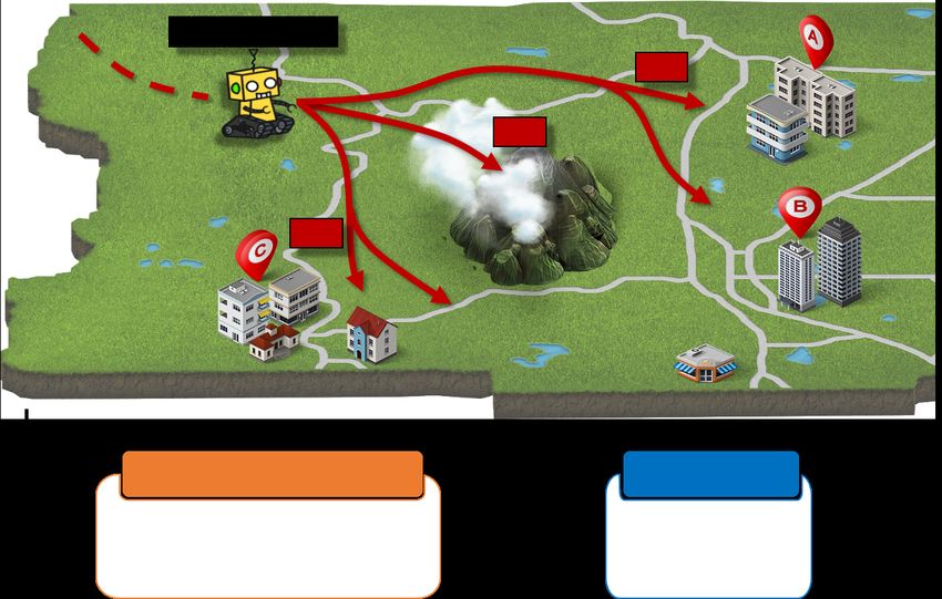
equal to ω(ci , c j ) if ((ci , qi ), (c j , q j )) ∈ δ rationality. For β = 0, the robot’s choice is just a uniformFig. 4. Example scenario of predictive monitoring for the robot that has an underlying intent ¬π0 ∧ ♦π2 ∧ ♦πg . The past five states (red circles) are
used for Bayesian intent inference and our monitor computes a distribution of future states (gray). The future trajectory is shown using small dots and the
ground truth of the future state is represented by red stars. As the robot navigates on the map, the monitor found π0 and pi1 are not a part of goals.
choice between all available moves regardless of the intent. to predict the possible future positions at a future time t + T .
However as β → ∞, the agent simply chooses the optimal Notice, however, that our model implicitly assumes that the
edge along the shortest cost path. With the appropriate robot’s intents change arbitrarily and are chosen afresh at
normalizing constant, we note that each step according to the posterior distribution.
a) Example Scenario: Fig. 4 shows an example sce-
exp (−β (ω(xt , xt+1 ) + C (xt+1 , ϕ j ))) nario of a robot in a workspace with four distinct regions
P(xt+1 |xt , ϕ j ) = . labeled with atomic propositions π0 , π1 , π2 and πg as shown
∑c∈next(xt ) exp (−β (ω(xt , c) + C (c, ϕ j )))
(2) by the highlighted rectangles in the figure. The underlying
Using Bayes rule, we can now compute the (unnormalized) (ground truth) intent is to avoid the region π0 , visit regions
posterior likelihood as follows: π2 and πg . The path taken by the robot is shown using the
red circles whereas the predicted future distribution is shown
P(ϕ j |xt , xt+1 ) ∝ P(xt+1 | xt , ϕ j ) × π(ϕ j ) . (3) using various shades of gray, the darker shade representing a
higher probability. The ground truth future position is shown
The posterior probability is calculated by normalizing this
using the red star.
over all hypothesized intents ϕ ∈ H . We will recursively
At time t = 1, having observed just two data points, the
update the prior at each step to yield the posterior at the
intent to avoid π0 is guessed by our monitor. However, at
next step. However, it is often useful to capture a change in
time t = 7, the robot is seemingly unable to distinguish
the intent at each step by means of an “ε-transition”:
between the competing goals of reaching/avoiding π1 , πg and
1 π2 . However, at this time, the monitor predicts a right turn
πt+1 (ϕ j ) = (1 − ε)P(ϕ j | xt , xt+1 ) + ε . (4)
|H | with a high probability though the robot’s direction of travel
The so-called ε transition simply weights down the posterior would indicate that it continues moving in a straight line in
by a factor 1 − ε and adds a uniform probability distribution the positive y direction.
with a constant weight ε. This method allows us to quickly At time t = 12, we see that the robot’s direction of travel
capture the new intent when an agent changes its intent makes the intent to reach π2 clear. Similarly, at time t =
during the operation. In our experiments, we fix ε = 0.3. 19, we see that the goal of reaching π1 or that of πg are
considered likely with πg being seen as more likely to be
E. Posterior Predictive Distribution the robot’s intended target.
Given the current posterior P(ϕ j |xt , xt+1 ) computed using Thus, we see how the robot’s future positions are predicted
Eq. (3), we wish to forecast the future position of the robot. accurately by our monitor even though the set of possible
We model the movement of the robot as a stochastic process: intents are restricted to simple safety-guarantee formulas.
1) Let initial position be xt+1 and the initial intent distri-
IV. E XPERIMENTAL R ESULTS
bution be given by the distribution πt+1 from Eq. (4).
2) At time t = t + k, update the current intent distribu- In this section, we evaluate the performance of our mon-
tion: πt+k+1 = (1 − ε)πt+k + ε Uniform(H ), wherein itoring approach on two datasets – a synthetic data set gen-
Uniform(H ) represents a uniform distribution over the erated by a Probabilistic Roadmap (PRM) motion planning
elements of the finite set H . algorithm that was used to plan paths satisfying randomly
3) Sample an intent ϕ j from πt+k+1 . generated ground truth “intents”, and the THÖR human
4) Sample xt+k+1 from the distribution P(xt+k+1 |xt+k , ϕ j ) trajectory dataset [29]. Using these, we will answer the
according to Eq. (2). following questions: (Q1) How does the prediction accuracy
Using the procedure above, we obtain samples of potential change as a prediction horizon increases? and (Q2) How does
future trajectories of the robot. We can use these trajectories the computation time depend on the prediction time horizon?Fig. 5. Example of the evaluation setup showing goal regions labeled
by atomic propositions and an underlying intent that seeks some subset
of the regions/avoids the rest. The revealed trajectory is shown using red
circles while the future trajectory is shown using dotted lines. Predicted Fig. 6. Prediction accuracy tested on various settings.
distribution of future states is shown in various shades of gray with darker
shades representing higher probabilities. TABLE I
C OMPUTATION TIME FOR OUR APPROACH , AS RECORDED ON A
M AC B OOK P RO WITH 2.6 GH Z I NTEL C ORE I 7 AND 16 GB RAM.
Each evaluation is performed over a map with K distin-
guished regions marked by atomic propositions π1 , . . . , πK . Map size 20×20 50×50 100×100
Product Automaton Construction
The hypothesized intents consist of 2K formulas, each of the (32 states in a Büchi automaton)
0.07 0.23 0.75
form j∈A ♦π j ∧ i∈B ¬πi wherein A ∩ B = 0/ and A ∪
V V
Bayesian Intent Inference
0.16 0.56 2.13
B = {1, . . . , K}. Each evaluation consists of a path followed with 32 hypotheses
300 Monte-Carlo Simulations
by the robot wherein the monitor predicts the probability (5 / 10 / 15 steps)
0.28 / 0.55 / 0.81
distribution of the positions 5, 10 and 15 steps ahead. A pre-
diction is deemed correct if the actual ground-truth position
is predicted by our monitor as having a probability ≥ 0.01. for the real-life human trajectory dataset is comparable with
The trajectories are generated using two approaches: that of the synthesized PRM dataset. This partly validates
PRM trajectories: We use a map with N × N grid cells the rationality hypothesis that underlies our work.
and place K random regions on the map. Next, we mark a Next, we consider an evaluation of the computation time.
randomly chosen subset of these regions as obstacles and The computational complexity of our approach dependes on
select the remaining regions as targets. We use the PRM the size of product automata and the number of hypotheses.
motion planner off the shelf to generate a plan that may not Table I reports the computation time for constructing product
necessarily be optimal, but is often close to being optimal. automata, checking 32 intents, and Monte-Carlo simulations
Our experiments vary N ∈ {20, 50, 100} and K ∈ {3, 5}. for various map sizes. We note that the computation times
THÖR Human Motion Dataset: This publicly available remain small even for a 100 × 100 grid and 32 intents each
dataset includes multiple human trajectory data recorded in with 32 Büchi automaton states.
a room of 8.4 × 18.8 meters [29]. The workspace consists
of five goal locations around the room and one obstacle V. C ONCLUSION
in the middle. Participants navigate between goals while Thus, we have demonstrated a framework for inferring
avoiding the obstacle. To use this dataset for our monitor, intents and predicting likely future positions of robots. Our
we converted the workspace to a 50 × 50 grid map, and framework can be extended in many ways including richer
discretized human trajectory data. Among all trajectories, we set of intents, alternative assumptions on how intents change
selected 277 segments at random for our evaluation. over time, incorporating richer agent dynamics, maps with
time-varying regions of interest, alternatives to the noisy
A. Evaluation of Accuracy and Computation Time
rationality model considered, and finally, intents governing
Fig. 6 shows that the prediction accuracy for the various multiple agents. We propose to study these problems using
datasets under varying prediction horizons. We note that the the rich framework of logic, automata and games combined
performance degrades as the prediction horizon grows, as with fundamental insights from Bayesian inference and ma-
expected. Nevertheless, our approach continues to provide chine learning.
useful information nearly 70% of the time on prediction
horizons that are 10 steps ahead. Furthermore, this accuracy ACKNOWLEDGMENTS
can be increased further by considering correlations of intents This work was funded in part by the US National Science
over time which is currently not performed in our approach. Foundation (NSF) under award numbers 1815983, 1836900
We also note that the accuracy degrades when more atomic and the NSF/IUCRC Center for Unmanned Aerial Systems
propositions are considered and thus more hypothesized (C-UAS). The authors thank Prof. Morteza Lahijanian for
intents are available. Finally, we notice that the accuracy helpful discussions.R EFERENCES International Conference on Robotics and Automation (ICRA). IEEE,
2019, pp. 739–745.
[1] M. Althoff and J. M. Dolan, “Online verification of automated road [22] G. Ferri, P. Stinco, G. De Magistris, A. Tesei, and K. D. LePage,
vehicles using reachability analysis,” IEEE Transactions on Robotics, “Cooperative autonomy and data fusion for underwater surveillance
vol. 30, no. 4, pp. 903–918, 2014. with networked auvs,” in 2020 IEEE International Conference on
[2] S. B. Liu, H. Roehm, C. Heinzemann, I. Lütkebohle, J. Oehlerking, Robotics and Automation (ICRA). IEEE, 2020, pp. 871–877.
and M. Althoff, “Provably safe motion of mobile robots in human [23] S. Choudhury, K. Solovey, M. J. Kochenderfer, and M. Pavone,
environments,” in 2017 IEEE/RSJ International Conference on Intel- “Efficient large-scale multi-drone delivery using transit networks,” in
ligent Robots and Systems (IROS). IEEE, 2017, pp. 1351–1357. 2020 IEEE International Conference on Robotics and Automation
[3] M. Koschi and M. Althoff, “Set-based prediction of traffic partici- (ICRA). IEEE, 2020, pp. 4543–4550.
pants considering occlusions and traffic rules,” IEEE Transactions on [24] Z. Manna and A. Pnueli, “A hierarchy of temporal properties,” in
Intelligent Vehicles, 2020. Proc. Principles of Distributed Computing (PODC). ACM, 1990, p.
[4] Y. Chou, H. Yoon, and S. Sankaranarayanan, “Predictive runtime mon- 377–410.
itoring of vehicle models using bayesian estimation and reachability [25] A. Shah, P. Kamath, J. A. Shah, and S. Li, “Bayesian inference of
analysis,” in 2020 IEEE/RSJ International Conference on Intelligent temporal task specifications from demonstrations,” in Advances in
Robots and Systems (IROS). IEEE, 2020. Neural Information Processing Systems, 2018, pp. 3804–3813.
[5] R. Peddi, C. D. Franco, S. Gao, and N. Bezzo, “A data-driven [26] J. Kim, C. Muise, A. Shah, S. Agarwal, and J. Shah, “Bayesian
framework for proactive intention-aware motion planning of a robot inference of linear temporal logic specifications for contrastive ex-
in a human environment,” in 2020 IEEE/RSJ International Conference planations.” in IJCAI, 2019, pp. 5591–5598.
on Intelligent Robots and Systems (IROS). IEEE, 2020. [27] M. Vazquez-Chanlatte and S. A. Seshia, “Maximum causal entropy
[6] A. Rudenko, L. Palmieri, M. Herman, K. M. Kitani, D. M. Gavrila, specification inference from demonstrations,” in International Confer-
and K. O. Arras, “Human motion trajectory prediction: A survey,” ence on Computer Aided Verification. Springer, 2020, pp. 255–278.
The International Journal of Robotics Research, vol. 39, no. 8, pp. [28] M. Vazquez-Chanlatte, S. Jha, A. Tiwari, M. K. Ho, and S. Seshia,
895–935, 2020. “Learning task specifications from demonstrations,” in Advances in
[7] J. F. Fisac, A. Bajcsy, S. L. Herbert, D. Fridovich-Keil, S. Wang, Neural Information Processing Systems, 2018, pp. 5367–5377.
C. Tomlin, and A. D. Dragan, “Probabilistically safe robot planning [29] A. Rudenko, T. P. Kucner, C. S. Swaminathan, R. T. Chadalavada,
with confidence-based human predictions,” in Robotics: Science and K. O. Arras, and A. J. Lilienthal, “Thör: Human-robot navigation data
Systems, 2018. collection and accurate motion trajectories dataset,” IEEE Robotics
[8] D. Fridovich-Keil, A. Bajcsy, J. F. Fisac, S. L. Herbert, S. Wang, A. D. and Automation Letters, vol. 5, no. 2, pp. 676–682, 2020.
Dragan, and C. J. Tomlin, “Confidence-aware motion prediction for [30] Z. Manna and A. Pnueli, Temporal Verification of Reactive Systems:
real-time collision avoidance1,” The International Journal of Robotics Specification, New York, 1992.
Research, vol. 39, no. 2-3, pp. 250–265, 2020. [31] C. Baier and J.-P. Katoen, Principles of Model Checking. MIT Press,
[9] A. Bajcsy, S. L. Herbert, D. Fridovich-Keil, J. F. Fisac, S. Deglurkar, 2008.
A. D. Dragan, and C. J. Tomlin, “A scalable framework for real-time [32] P. Wolper, “Constructing automata from temporal logic formulas: a tu-
multi-robot, multi-human collision avoidance,” in 2019 international torial,” in Lectures on formal methods and performance analysis: first
conference on robotics and automation (ICRA). IEEE, 2019, pp. EEF/Euro summer school on trends in computer science. Springer,
936–943. 2002, pp. 261–277.
[10] G. Best and R. Fitch, “Bayesian intention inference for trajectory [33] W. Thomas, “Automata on infinite objects,” in Handbook of Theo-
prediction with an unknown goal destination,” in 2015 IEEE/RSJ retical Computer Science: Volume B: Formal Models and Semantics,
International Conference on Intelligent Robots and Systems (IROS). J. van Leeuwen, Ed. Amsterdam: Elsevier, 1990, pp. 133–191.
IEEE, 2015, pp. 5817–5823. [34] P. Gastin and D. Oddoux, “Fast ltl to büchi automata translation,” in
[11] B. I. Ahmad, J. K. Murphy, P. M. Langdon, and S. J. Godsill, International Conference on Computer Aided Verification. Springer,
“Bayesian intent prediction in object tracking using bridging distribu- 2001, pp. 53–65.
tions,” IEEE transactions on cybernetics, vol. 48, no. 1, pp. 215–227, [35] A. Duret-Lutz, A. Lewkowicz, A. Fauchille, T. Michaud, E. Renault,
2016. and L. Xu, “Spot 2.0 — a framework for LTL and ω-automata
[12] I. Hwang and C. E. Seah, “Intent-based probabilistic conflict detection manipulation,” in International Symposium on Automated Technology
for the next generation air transportation system,” Proceedings of the for Verification and Analysis. Springer, 2016, pp. 122–129.
IEEE, vol. 96, no. 12, pp. 2040–2059, 2008. [36] B. D. Ziebart, A. L. Maas, J. A. Bagnell, and A. K. Dey, “Maximum
[13] J. L. Yepes, I. Hwang, and M. Rotea, “New algorithms for aircraft in- entropy inverse reinforcement learning.” in Aaai, vol. 8. Chicago, IL,
tent inference and trajectory prediction,” Journal of guidance, control, USA, 2008, pp. 1433–1438.
and dynamics, vol. 30, no. 2, pp. 370–382, 2007.
[14] A. Bhatia, L. E. Kavraki, and M. Y. Vardi, “Sampling-based motion
planning with temporal goals,” in 2010 IEEE International Conference
on Robotics and Automation. IEEE, 2010, pp. 2689–2696.
[15] ——, “Motion planning with hybrid dynamics and temporal goals,”
in 49th IEEE Conference on Decision and Control (CDC). IEEE,
2010, pp. 1108–1115.
[16] G. E. Fainekos, A. Girard, H. Kress-Gazit, and G. J. Pappas, “Temporal
logic motion planning for dynamic robots,” Automatica, vol. 45, no. 2,
pp. 343–352, 2009.
[17] H. Kress-Gazit, G. E. Fainekos, and G. J. Pappas, “Temporal-logic-
based reactive mission and motion planning,” IEEE transactions on
robotics, vol. 25, no. 6, pp. 1370–1381, 2009.
[18] L. R. Humphrey, E. M. Wolff, and U. Topcu, “Formal specification
and synthesis of mission plans for unmanned aerial vehicles,” in 2014
AAAI Spring Symposium Series, 2014.
[19] C. I. Vasile and C. Belta, “Reactive sampling-based temporal logic
path planning,” in 2014 IEEE International Conference on Robotics
and Automation (ICRA). IEEE, 2014, pp. 4310–4315.
[20] A. Ulusoy, S. L. Smith, X. C. Ding, C. Belta, and D. Rus, “Optimality
and robustness in multi-robot path planning with temporal logic
constraints,” The International Journal of Robotics Research, vol. 32,
no. 8, pp. 889–911, 2013.
[21] V. L. Somers and I. R. Manchester, “Priority maps for surveillance
and intervention of wildfires and other spreading processes,” in 2019You can also read