Flight Planning for Unmanned Aerial Vehicles - AMOS # 34(2015) Angewandte Mathematik und Optimierung Schriftenreihe Applied Mathematics and ...
←
→
Page content transcription
If your browser does not render page correctly, please read the page content below
Angewandte Mathematik und Optimierung Schriftenreihe
    Applied Mathematics and Optimization Series
                 AMOS # 34(2015)

Armin Fügenschuh and Daniel Müllenstedt

Flight Planning for Unmanned Aerial Vehicles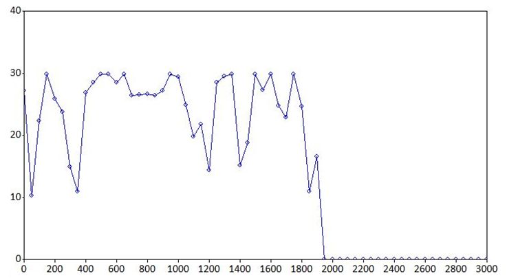
Herausgegeben von der
Professur für Angewandte Mathematik
Professor Dr. rer. nat. Armin Fügenschuh

Helmut-Schmidt-Universität / Universität der Bundeswehr Hamburg
Fachbereich Maschinenbau
Holstenhofweg 85
D-22043 Hamburg

Telefon: +49 (0)40 6541 3540
Fax: +49 (0)40 6541 3672

e-mail: appliedmath@hsu-hh.de
URL: http://www.hsu-hh.de/am

Angewandte Mathematik und Optimierung Schriftenreihe (AMOS), ISSN-Print 2199-1928
Angewandte Mathematik und Optimierung Schriftenreihe (AMOS), ISSN-Internet 2199-1936
Flight Planning for Unmanned Aerial Vehicles

                             Armin Fügenschuh 1
    Helmut Schmidt University / University of the Federal Armed Forces Hamburg
                       Holstenhofweg 85, 22043 Hamburg

                             Daniel Müllenstedt 2
    Helmut Schmidt University / University of the Federal Armed Forces Hamburg
                       Holstenhofweg 85, 22043 Hamburg

Abstract
We formulate the mission planning problem for a fleet of unmanned aerial vehicle
(UAV) as a mixed-integer nonlinear programming problem (MINLP). The problem
asks for a selection of targets from a list to the UAVs, and trajectories that visits
the chosen targets. To be feasible, a trajectory must pass each target at a desired
distance and within a certain time windows, obstacles or regions of high risk must be
avoided, and the fuel limitations must be obeyed. An optimal trajectories maximizes
the sum of values of all targets that can be visited, and as a secondary goal, conducts
the mission in the shortest possible time. In order to obtain numerical solutions
to this model, we approximate the MINLP by an mixed-integer linear program
(MILP), and apply state-of-the-art solvers (Cplex, Gurobi) to the latter on a set of
test instances.
Keywords: Mixed-Integer Nonlinear Programming, Trajectory Planning,
Unmanned Aerial Vehicles, Approximation.

1
    Email: fuegenschuh@hsu-hh.de
2
    Email: daniel.muellenstedt@hsu-hh.de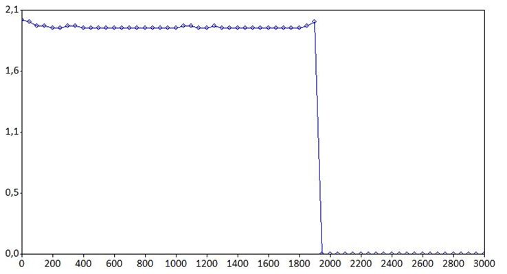
1   Introduction
The mission planning problem for an unmanned aerial vehicle (UAV) asks
for an optimal trajectory that visits a largest possible subset from a list of
desired targets. When selected, each target must be traversed in a certain
maximal distance and within a certain time interval. In a further variant of this
problem, a fleet of potentially inhomogeneous UAVs is given. The UAVs differ
with respect to their sensor properties, radar profiles, and operating ranges.
Before actually planning the trajectories, a vehicle-to-target assignment has
to be carried out. If the targets are surrounded by radar surveillance, then the
vehicles trajectory should be chosen to minimize the risk of detection. Hereto,
the flight trajectory should make use of terrain properties. This planning
problem is similar to classical vehicle routing problems with time windows
(VRPTW) that are analyzed in the field of Operational Research. However,
in these models the vehicles only move on a street network that is modeled
as a graph. The UAV in contrast can fly freely through the three dimensional
space. Moreover the fuel consumption for road based vehicles (cars or lorries)
is more easy to calculate compared to UAVs. For the latter, the current weight,
the altitude, the speed and climb/descend have an influence on the actual fuel
consumption. Furthermore, the aspect of risk (of being detected) during the
flight does not occur in classical VRPTW models. We formulate the mission
planning problem for UAVs as mixed-integer linear nonlinear programming
problem. Binary decision variables are used to represent the decision about
which target is inspected by which vehicle at which time. If too many targets
are specified, then the model selects the most valuable ones with respect to a
predefined ordering of the targets, where a target scoring function for visited
targets is given. There are two conflicting criteria for the optimization of
the trajectory, namely to maximize the sum of scores for visited targets, and
to minimize the probability of getting caught by the adversary’s radar. We
formulate this optimization problem as a mixed-integer programming problem
and solve it numerically using available solver software. To compute the Pareto
front we solve a sequence of optimization problems with varying coefficients
in the objective function.

2   Survey of the Literature
The desire for unmanned aerial vehicles (UAVs) is as old as the history of
human flight itself. For historical surveys we refer to [23,3,17]. During the
last 15 years their popularity for use in military and civil applications rose.
This reflects in the number of scientific publications over the past two decades
that focus on the deployment of UAVs. From a mathematical or operations
research point-of-view, roughly speaking, one can cluster the approaches by
their degree of details on physical and technical properties that is incorporated
into the models. On the one side, there exist highly detailed models that try
to describe the physical properties of a flying UAV as accurate as possible,
see for instance [19,26]. Such models can be used to control a UAV for a
very short segment of its trajectory. The numerical effort for solving such
models does not allow to incorporate decisions on selecting targets or the
ordering. On the other side of the range there are models that ignore most of
the physical properties or approximate them in a very coarse way. Here, for
example, the UAV is flying only in standard altitude and with standard speed,
and the fuel consumption is assumed to be constant over time. Because they
ignore the physics of flight such models, as the VRPTW mentioned above,
can include a large number of targets and vehicles and can still be solved
to proven global optimality [24,10]. Between these two extremal sides, there
are numerous publications that include several aspects of the real-world in
order to be realistic, while neglect other aspects to become solvable. In the
following, we review some of them.
    Ma et al. [22] use an ant colony metaheuristic strategy to find a trajectory
for a single UAV that traverses towards a single target point and must avoid
threat points where the UAV might be detected by radar. The trajectory is
smoothed in a post-processing step to reflect turn constraints. Fuel is not
considered, and the trajectory is planar (2D).
    Schøler [27] work is based on visibility graphs in 3D that are used for UAV
path planning. He focuses on the collision free path planning around obstacles
with minimum length.
    Cobano et al. [6] use a genetic algorithm to solve a trajectory planning
problem for multiple UAVs that avoids collisions.
    Borelli et al. [4] address the conflict resolving problem for multiple UAVs.
They numerically compare a nonlinear programming formulation with a mixed-
integer linear formulation and demonstrate that the latter is faster the more
dominant the disjunctive constraints become.
    Robustness aspects for a single UAV are included in the work of Luders
[21], that is, the trajectory should still be feasible when small disturbances to
the input data occurs. Hereto a linear dynamic model for the vehicle motion is
assumed, and the whole problem is thus a mixed-integer linear program that
can be numerically solved via Cplex.
    Gao et al. [13] use Dubins curve to describe the path of a UAV. A Dubins
path is the shortest curve that connects two points in the 2D plane subject to
further constraints on the curvature of the path and given initial and terminal
tangents to the path [8].
For a given set of waypoints, Forsmo [11] considers 2D path planning for
a single UAV with mixed-integer linear programming, where flying around
static rectangular obstacles is taken into account. Nonlinear constraints are
approximated by piece-wise linear ones. The MILP problems are solved with
Gurobi.
The focus of Evers et al. [9] is on robustness and uncertainty. They use
a graph to model the dynamic of the UAV, similar to the traveling salesman
problem, thus flight physics are neglected. However, their approach allows to
cover online aspects, when new waypoints emerge during the flight.
Geiger et al. [14] use a direct collocation method and approximate the
trajectory for single or multiple UAVs by piecewise polynomials. The goal
is not to minimize the flight time (as in most other publications), but to
maximize the viewing time for the mounted sensor devices. The target can be
stationary or moving, and wind can be taken into account.
Ruz et al. [25] take a symmetric adversary into account that uses radar to
detect UAVs. Hence they describe a radar model and plan a trajectory that
avoids areas of high detection risk. Their model is formulated as a mixed-
integer linear program, and applied to a single target and a single UAV.
Lee et al. [20] consider the problem of following a moving ground vehicle
with a UAV. If the ground vehicle is slower than the UAV, the path slingers
around the ground vehicle’s trajectory in a sinusoidal mode. When the vehicle
stops, the UAV is performing a rose-shaped curve during its loitering mode.
The switching between these two modes is performed ad-hoc in an online way,
depending on the changing behavior of the ground vehicle. Thus no integer
model is formulated and solved.
Jun and D’Andrea [16] give a graph-based formulation for the UAV path
planning problem that can be solved by shortest-path algorithms (Dijkstra
or Bellman-Ford). Sharp edges of the trajectory are smoothed in a post-
processing step. The area is discretized, and each finite cell area is endowed
with a risk value (a probability map). The objective is to find a risk-minimal
path from an origin to a target for single UAV.
Culligan [7] studies the online trajectory planning problem for UAVs, and
formulates this problem as a mixed-integer program. The nonlinear kinematic
constraints are linearized by piecewise linear approximation. Obstacles are
modeled by rectangular boxed in 3D and avoidance constraints are formulated
by binary variables. In a similar way, cost regions are formulated. Obstaclescan be static or dynamic. The earth’s surface shape can be taken into account
to allow flights close to the surface.
A different approach is presented by Kress and Royset [18], where the
targets are unknown at the beginning of the mission and should be detected by
a fleet of UAVs. The targets move around the area with certain probabilities.
The goal is to determine a search plan that specifies which part of the area is
searched in which (discretized) time period. This problem can be modeled as
a mixed-integer linear problem, and is solved using Cplex within 2 minutes.
The physical and technical properties of actual UAVs are mostly ignored. Only
collision avoidance constraints and a maximum deployment time is considered.
We contribute to the state of the art by presenting a model that simultane-
ously takes into account several aspects of the mission and trajectory planning
process that were treated independently before: Our model is capable to plan
a 4D path (3D in space plus time) around static or dynamic obstacles. The
fuel consumption of the UAVs is considered. The selection of spaces and their
assignment to the fleet of UAVs is part of the model, as well as the ordering
in which the chosen places are to be visited.
3 A Mathematical Model
We first formulate the UAV trajectory planning problem as a mixed-integer
nonlinear program, and reformulate it later as a mixed-integer linear program.
In the following, k · k denotes the Euclidean norm in R2 or R3 . We denote
1 := (1, 1, 1).
3.1 Sets
The following sets describe an instance of the problem.
Given is a set of UAVs U := {1, . . . , U }, a set of waypoints W := {1, . . . , W },
a set of restricted air spaces Q := {1, . . . , Q}, a set of atmospheric layers
L := {1, . . . , L}, and a set of discrete time steps T := {0, . . . T }. As abbrevi-
ations we set T − := T \{T }, and L := L ∪ {0}.
3.2 Parameters
The following parameters need to be specified. They describe the technical
and geographical environment of the mission.3.2.1 UAV Technical Parameters
The minimum and maximum velocity of UAV u are denoted by v u , v u ∈ R+ .
Its maximum acceleration is au ∈ R+ , and its maximum flight altitude is hu .
The minimum safety distance between two airborne UAVs to avoid collisions
is ε = (εx , εy , εz ) ∈ R3+ .
The initial fuel at start is denoted by Ku ∈ R+ . We assume a layer model
for the fuel consumption. For this we define layer boundaries H0 < H1 <
. . . < HL . The value H0 is (close to) zero, and HL is the maximum flight
altitude of the UAVs. Then ηu,l , ξu,l ∈ R+ are fuel consumption parameters
for UAV u in layer l ∈ L.
3.2.2 Mission Parameters
The start and end location for each UAV u are the coordinate vector R0u , RTu ∈
R3 . A number of waypoints pw ∈ R3 is given that should all be visited, if time
and fuel conditions allow. Depending on the sensor/actor technique and the
desired goal, a maximal operational distance to the waypoint w for UAV u
is given by `u,w . When reaching a waypoint within the prescribed distance,
a score value sw is added to the objective. Each waypoint must be reached
within a time window Tw ⊆ T .
The ground control station for UAV u is located at the coordinates g u =
(gux , guy , 0) ∈ R3 , and the UAV can be controlled up to a maximum distance
Ru . Hereby we assume that there are no obstacles to the line-of-sight in all
directions. Otherwise, one can specify those regions without connection as
restricted air spaces.
3.2.3 Environmental Parameters
Restricted air spaces are three dimensional rectangular regions that are not
allowed to be entered by the UAV. This feature can be used to capture regions
without connection between the UAV and the ground control station, moun-
tains or high buildings, or adversary radar or air defense systems. For each
restricted air space q ∈ Q a vector of its lower and upper bound coordinates
is specified: cq (t), cq (t) ∈ R3 . Each restricted airspace may vary its location
over time t.
The wind velocity is given by w(t) = (wx (t), wy (t), wz (t)) ∈ R3 . Hereby
we assume that wind may vary over time, but is constant for the whole flight
area.3.3 Variables
The trajectory for each UAV u ∈ U is described by a set of coordinate vec-
tors (continuous variables) r u (t) = (rux (t), ruy (t), ruz (t)) ∈ R3 for each discrete
time t ∈ T . The velocity of vehicle u at time t is denoted by the continuous
variables v u (t) = (vux (t), vuy (t), vuz (t)) ∈ R3 , and its acceleration is modeled
by the continuous variables au (t) = (axu (t), ayu (t), azu (t)) ∈ R3 . The binary
variables bu (t) ∈ {0, 1} indicate if UAV u is airborne in time step t. The
binary variables du,w (t) ∈ {0, 1} indicate if UAV u reaches waypoint w at time
step t ∈ Tw . The binary variables f u,q (t) = (f xu,q (t), f yu,q (t), f zu,q (t)), f u,q (t) =
x y z
(f u,q (t), f u,q (t), f u,q (t)) ∈ {0, 1}3 for each u ∈ U, q ∈ Q model if the vehicle is
within a restricted airspace. The binary variables eu,u0 (t) = (exu,u0 (t), eyu,u0 (t), ezu,u0 (t)),
eu,u0 (t) = (exu,u0 (t), eyu,u0 (t), ezu,u0 (t)) ∈ {0, 1}3 for u, u0 ∈ U, u < u0 and t ∈ T
model if vehicle u is too close to u0 with respect to safety requirements. The
binary variables hu,l (t) ∈ {0, 1} describe if UAV u is flying in layer l ∈ L0 in
time step t. The layer l = 0 means the aircraft is landed and the engine is off
(in particular, no fuel consumption). The continuous variables Ku,l (t) ∈ R+
represent the fuel consumption when flying in layer l at time step t. The con-
tinuous variables ku (t) ∈ R+ then represent the fuel consumption of vehicle u
at time step t. The continuous variables mu (t) ∈ R+ that describe the amount
of fuel on board of UAV u at time step t.
3.4 Constraints
The following constraints define a feasible assignment of waypoints to UAVs
and the UAV flight itself.
3.4.1 Flight Area
The flight starts and ends for each UAV at the specified coordinates:
r u (0) = R0u , ∀ u ∈ U, (1)
r u (T ) = RTu , ∀ u ∈ U. (2)
The UAV must keep a connection to the ground control unit (otherwise, an
emergency landing procedure is initiated). Hence a range limit is imposed:
kr u (t) − g u k ≤ Ru , ∀ u ∈ U, t ∈ T . (3)
The altitude cannot be higher than the maximum altitude:
ruz (t) ≤ hu , ∀ u ∈ U, t ∈ T . (4)3.4.2 Flight Dynamics
The flight dynamic is described by a point model for the UAV [5]. By Newton’s
law of motion we have that the acceleration as the derivative of the velocity,
and the velocity as the derivative of the location:
dv d2 r
a= = 2.
dt dt
Since we are discretizing the time and use a finite difference approach, New-
ton’s law enters our model in the following form. The position is updated by
a second order difference equation, where the influence of wind is also taken
into account:
(∆t)2
r u (t + 1) = r u (t) + ∆t · (v u (t) + w(t)) + · au (t), ∀ u ∈ U, t ∈ T − . (5)
2
The velocity is updated by a first order difference equation:
v u (t + 1) = v u (t) + ∆t · au (t), ∀ u ∈ U, t ∈ T − . (6)
The velocity is limited by certain lower and upper bounds:
v u ≤ kv u k, ∀ u ∈ U, (7)
kv u k ≤ v u , ∀ u ∈ U. (8)
The acceleration is only limited from above:
kau k ≤ au , ∀ u ∈ U. (9)
The following constraints take control of the in-air time of each UAV:
kr u (t) − RTu k ≤ M · bu (t), ∀ u ∈ U, t ∈ T − . (10)
Here and in the sequel M ∈ R+ is a sufficiently large value. If the flight is
terminated in some time step t, it remains terminated for the remainder of
the finite time horizon, that is, the UAV cannot start immediately again:
bu (t + 1) ≤ bu (t), ∀ u ∈ U, t ∈ T − . (11)
3.4.3 Waypoints
If a waypoint w ∈ W is met, then the UAV must fly by in a certain maximal
distance:
kr u (t) − pw k ≤ `u,w + M · (1 − du,w (t)), ∀ u ∈ U, w ∈ W, t ∈ W. (12)At most one UAV can claim a waypoint:
X
du,w (t) ≤ 1, ∀ w ∈ W. (13)
u∈U ,t∈Tw
3.4.4 Restricted Airspaces
A rectangular area where the UAV is not allowed to fly through is modeled
as follows:
cq (t) − M · f u,q (t) ≤ r u (t), ∀ u ∈ U, q ∈ Q, t ∈ T , (14)
r u (t) ≤ cq (t) + M · f u,q (t), ∀ u ∈ U, q ∈ Q, t ∈ T , (15)
1 · f u,q (t) + 1 · f u,q (t) ≤ 5, ∀ u ∈ U, q ∈ Q, t ∈ T . (16)
Constraints (14), (15) require that if the UAV u is staying inside the forbidden
box [cxq , cxq ] × [cyq , cyq ] × [czq , czq ], then all six binary variables from f u,q (t) and
f u,q (t) must be set to 1, which is forbidden by constraints (16).
3.4.5 Collision Avoidance
If U > 1, i.e., more than one UAV is flying at the same time, then for each
pair of UAVs u, u0 ∈ U with u < u0 it has to ensured that their trajectories are
sufficiently separated in order to avoid a collision. In a way each UAV defines
a restricted airspace that no other UAV must enter:
r u0 (t) + ε − M · eu,u0 (t) ≤ r u (t), ∀ u, u0 ∈ U : u < u0 , t ∈ T , (17)
r u (t) ≤ r u0 (t) − ε + M · eu,u0 (t), ∀ u, u0 ∈ U : u < u0 , t ∈ T , (18)
1 · eu,u0 (t) + 1 · eu,u0 (t) ≤ 5, ∀ u, u0 ∈ U : u < u0 , t ∈ T . (19)
3.4.6 Fuel Consumption
We use an approximative fuel consumption model that takes into account
several atmospheric layers. In general, the higher the altitude the less fuel
is consumed by the UAV. Moreover, the higher the velocity, the more fuel it
consumes. First, we detect the altitude layer and switch the corresponding
binary variable:
X X
Hl−1 · hu,l (t) ≤ ruz (t) ≤ Hl · hu,l (t), ∀ u ∈ U, t ∈ T . (20)
l∈L l∈LExactly one layer is active:
X
hu,l (t) = 1, ∀ u ∈ U, t ∈ T . (21)
l∈L0
The fuel consumption in layer l then depends on the velocity of the UAV. We
assume an affine-linear relationship:
Ku,l (t) = ηu,l + ξu,l · kv u (t)k, ∀ u ∈ U, l ∈ L, t ∈ T . (22)
The fuel consumption variable ku (t) is assigned with the value of the auxiliary
variable Ku,l (t), if and only if the UAV u is in the layer l:
Ku,l (t) − M · (1 − hu,l (t)) ≤ ku (t), ∀ u ∈ U, l ∈ L, t ∈ T , (23)
ku (t) ≤ Ku,l (t) + M · (1 − hu,l (t)), ∀ u ∈ U, l ∈ L, t ∈ T . (24)
At start, the UAV’s fuel level is initialized with the start fuel amount:
mu (0) = Ku , ∀ u ∈ U. (25)
During the flight, the fuel is reduced according to the above computed amount:
mu (t + 1) = mu (t) − ku (t), ∀ u ∈ U. (26)
3.5 Objective
The primary goal is to maximize the score for reaching the waypoints. On a
subordinate level it is desired to finish the mission as soon as possible. This
reflects the following objective function:
X 1 X
max sw · du,w (t) − bu (t). (27)
u∈U ,w∈W,t∈Tw
M u∈U ,t∈T
4 Linearizing the Model
The model contains several nonlinear constraints. In order to apply a linear
mixed-integer solver, we linearize them and thus obtain an approximation.
4.1 Second Order Cone Approximation
All nonlinear constraints in the model – (3), (7), (8), (9), (10), (12), (22) –
involve the Euclidean norm k · k. Moreover, in almost all nonlinear constraintsthis norm is bounded from above, with (7) being the only exception. In
these cases we can approximate the nonlinear constraint by a second order
cone approximation introduced by Ben-Tal and Nemirovski [1] and refined by
Glineur [15]. The presented approach is similar to Yuan et al. [28] for the
free-flight problem in civil airplane trajectory planning.
4.1.1 SOC in 3D
The case of three dimensions can be p reduced to the two dimensional case as
follows. Assume that a generic cone x21 + x22 + x23 ≤ z (with x1 , x2 , x3 ∈ R
and z ∈ R+ ) should p be approximated. p Then we approximate the two two-
dimensional cones x21 + x22 ≤ y and y 2 + x23 ≤ z.
From the first cone we get by squaring both sides: x21 + x22 ≤ y 2 , and from
the second cone we get y 2 + x23 ≤ z 2 , or equivalently y 2 ≤ z 2 − x23 . Putting
these two together gives x21 + x22 ≤ y 2 ≤ z 2 − x23 , which is x21 + x22 + x23 ≤ z 2 .
Taking the square roots on both sides gives the desired three dimensional conic
equation.
4.1.2 SOC in 2D
It remains to approximate
p second order cones in two dimensions. A generic
2 2
cone is given by x1 + x2 ≤ z. In order to achieve a linear approximation it
is of course possible to approximate the Lorentz cone directly in R3 by linear
hyperplanes. Note that this means to approximate a circle with diameter z
by piecewise linear segments, an ancient idea that can be dated back at least
to the greek scientist Archimedes of Syracuse (287 BC – 212 BC). Archimedes
used this method to numerically approximate π, see Berggren et al. [2] and
the references therein. However, this approximation is known to converge very
slowly. In general one can prove that the approximation error, i.e., the largest
deviation between a circle and an outer approximating regular polygon with
J sides is given by
π −1
ε = cos − 1, (28)
J
(cf. Theorem 2.1 in Glineur [15]). For an accuracy of 10−4 we thus would
already need a 223-gon. Each of these sides corresponds to a linear hyperplane.
In order to achieve even an only modest approximation of the Lorentz cone we
would thus need already a high number of facets, which leads to high running
times for the numerical MILP solver and also numerical problems when solved
the LP-relaxations, since the angle between these hyperplanes is almost 180
degree [12].
A much better approximations of the Lorentz cone is achieved by a pro-jection in a higher-dimensional settings, which was first given by Ben-Tal and
Nemirovski [1]. We use a slightly improved version of their result, given by
Glineur [15]. To this end we introduce auxiliary variables αi,j , βi,j ∈ R for
1 ≤ i ≤ n and j = 0, 1, . . . , J, where J is called approximation level, and
takes control of the quality of the approximation. We then add the following
constraints to the model for all 1 ≤ i ≤ n:
αi,0 = x1 , (29a)
βi,0 = x2 , (29b)
π π
αi,j+1 = cos · αi,j + sin j · βi,j , ∀ j = 0, . . . , J − 1, (29c)
2j 2
π π
βi,j+1 ≥ − sin j · αi,j + cos j · βi,j , ∀ j = 0, . . . , J − 1, (29d)
π 2 π 2
βi,j+1 ≥ sin j · αi,j − cos j · βi,j , ∀ j = 0, . . . , J − 1, (29e)
2π 2π
z = cos J · αi,J + sin J · βi,J . (29f)
2 2
In [1,15] it is shown that the approximation error is
π −1
ε = cos − 1. (30)
2J
Hence, to achieve the same accuracy of 10−4 as above (for approximating the
Lorentz cone, that is), we need (29) with J = 8, which means 2 · J = 16
additional variables and 3 · J + 3 = 27 additional constraints (see also [12]).
4.2 Minimum Velocity
The SOC approximation is only valid if an upper bound constraint is imposed
on the Euclidean norm. A lower bound constraint leads to a non-convex
feasible region, and thus needs to be treated by further binary variables in
order to deal with this disjunction. This applies to constraints (7) in our
model. Small velocities are excluded in the same way as restricted air spaces,
where additional binary variables are introduced to refrain the velocity from
being smaller than v. Note that this gives only a rectangular box around the
origin, which is a rather coarse approximation in comparison with the upper
bound, where the round shape of the boundary was approximated which a
much higher precision due to the convexity and the SOC property.No. W Q U T vars. int. cons.
1 3 1 1 61 7992 1037 11101
2 3 2 1 61 8358 1403 11528
3 3 1 2 61 16349 2440 22625
4 3 2 2 61 17081 3172 23479
5 6 1 2 61 24035 2806 90965
6 8 2 2 61 29891 3782 41164
7 10 3 2 61 35747 4758 49092
8 15 0 1 61 22998 1403 31902
Table 1
Instance data.
5 Computational Results
The linearized version of the above model is a mixed-integer linear program-
ming problem. We generated a test set of eight instances that vary in the
size in terms of number of waypoints W , number of restricted areas Q, and
number of UAVs U . The size thus also varies in terms of number of vari-
ables, integer variables, and constraints (see Table 1). All instances have a
time horizon of 3000 seconds and a time discretization of ∆t := 50 seconds,
which leads to T := 61 time steps. These instances were generated with the
modeling language AIMMS (Version 4.9) and solved using the state-of-the-art
MILP solvers Gurobi (Version 6.0) (see Table 2) and Cplex (Version 12.6.2)
(see Table 3). A time limit of 3600 seconds was imposed for each run, and
default settings were used for both solvers. The hardware environment we
used was a Windows Laptop running an Intel Core i7 at 2.40 GHz clock speed
and 16 GB RAM. Within this time limit, instances #1 to #6 could be solved
to proven global optimality. For the largest two instances #7 and #8 there
remained a gap (i.e., a difference between the best primal solution and the
dual bound). The results are visualized using AIMMS again. One example of
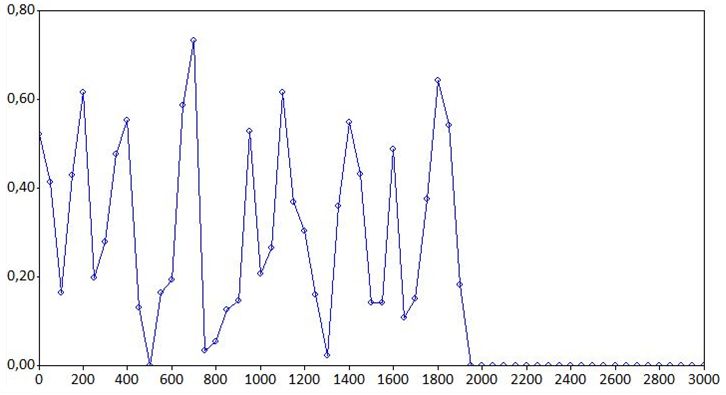
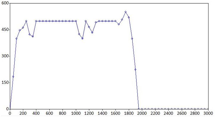
this is shown in Figure 1-5, which corresponds to the solution of instance #6.
Another example with two UAVs is shown in Figure 6.
6 Conclusions
We studied the flight trajectory and mission planning problem for a fleet of
UAVs and gave a mixed-integer nonlinear formulation. We demonstrated how
to approximate it by piecewise linear constraints that rely on second order cone
approximations. Numerical tests revealed what instance sizes current state-No. time iter. nodes primal dual
1 57 416878 1434 5.943606286 5.943606286
2 127 1007749 2935 5.93158997 5.93158997
3 423 1851334 4512 5.92135216 5.92135216
4 963 3435349 6529 5.91145625 5.91145625
5 2089 11860777 11209 11.76989656 11.76989656
6 3276 12919437 22301 15.96719977 15.96719977
7 3600 10532839 18214 17.77854903 19.92483253
8 3600 10451122 15833 13.86587307 27.87871092
Table 2
Gurobi results.
No. time iter. nodes primal dual
1 153 877231 2264 5.93413156 5.93413156
2 286 1431425 3213 5.92251567 5.92251567
3 642 3212314 4865 5.952242493 5.952242493
4 1042 4531346 6783 5.944526896 5.944526896
5 2217 12001345 10984 11.771351 11.771351
6 3417 13511315 22487 15.96813145 15.96813145
7 3600 11123514 14647 15.7123478 19.93541258
8 3600 11860777 12209 11.76989656 29.73958682
Table 3
Cplex results.
of-the-art MILP solvers are able to handle on standard desktop computer
hardware. It turned out that Gurobi is significantly faster than Cplex on our
test instances. Still, the instance size that can be solved with this approach
is currently rather small.
Our future work focuses on developing techniques to solve larger instances.
The development of problem specific heuristics can help to find good solutions
faster. On the dual side, a decoupling of the assignment process from the
trajectory planning step is a promising direction for future work.
Acknowledgement. This research was supported by the BMBF project “E-
Motion”. We thank our colleagues from the Planungsamt der Bundeswehr, Otto-
brunn, and from the Aufklärungslehrbataillon 3, Lüneburg, for fruitful discussions.Fig. 1. Visualization of the solution to instance #6. S-1, S-2 are the start/end
locations for the UAV’s trajectories. W-1, . . . , W-8 are the waypoints. F-1, F-2 are
restricted airspaces. (Background image source: GoogleMaps.)
Fig. 2. Velocity over time in the solution to instance #6.
References
[1] Aaron Ben-Tal and Arkadi Nemirovski. On polyhedral approximations of the
second-order cone. Mathematics of Operations Research, 26(2):193–205, 2001.
[2] L. Berggren, J. Borwein, and P. Borwein. Pi: A Source Book. Springer Verlag,Fig. 3. Acceleration over time in the solution to instance #6.
Fig. 4. Altitude over time in the solution to instance #6.
New York, 1997.
[3] J. D. Blom. Unmanned Aerial Systems : a historical perspective. Technical
report, Combat Studies Institute Press, US Army Combined Arms Center, Fort
Leavenworth, Kansas, 2010.
[4] Francesco Borrelli, Dharmashankar Subramanian, Arvind U. Raghunathan, and
Lorenz T. Biegler. MILP and NLP Techniques for Centralized Trajectory
Planning of Multiple Unmanned Air Vehicles. In IEEE American Control
Conference 2006, Minneapolis, MN, 2006.
[5] E. Brommundt, G. Sachs, and D. Sachau. Technische Mechanik - Eine
Einführung. Oldenbourg Wissenschaftsverlag GmbH, 2007.
[6] J. A. Cobano, D. Alejo, R. Conde, and A. Ollero. A new method for UAVFig. 5. Fuel consumption per time step in the solution to instance #6. Fig. 6. Visualization of the solution to instance #7. (Background image source: GoogleMaps.) trajectory planning under uncertainties. In Proceedings of the Workshop on Research, Development and Education on Unmanned Aerial Systems (RED- UAS). Seville, November 30 and December 1, 2011.
[7] Kieran Forbes Culligan. Online Trajectory Planning for UAVs Using Mixed
     Integer Linear Programming. Master’s thesis, Massachusetts Institute of
     Technology, Department of Aeronautics and Astronautics, 2006.

 [8] L. E. Dubins. On Curves of Minimal Length with a Constraint on Average
     Curvature, and with Prescribed Initial and Terminal Positions and Tangents.
     American Journal of Mathematics, 79(3):497–516, 1957.

 [9] Lanah Evers, Ana Isabel Barros, Herman Monsuur, and Albert Wagelmans.
     UAV Mission Planning: From Robust to Agile. In Vasileios Zeimpekis, George
     Kaimakamis, and Nicholas J. Daras, editors, Military Logistics, Interfaces Series
     56, pages 1–17. Springer International Publishing, Switzerland, 2015.

[10] Mariam Faied, Ahmed Mostafa, and Anouck Girard. Vehicle Routing Problem
     Instances: Application to Multi-UAV Mission Planning. In AIAA Guidance,
     Navigation, and Control Conference, 2 - 5 August 2010, Toronto, Ontario
     Canada, 2010.

[11] Erik Johannes Forsmo. Optimal Path Planning for Unmanned Aerial Systems.
     Master’s thesis, Norwegian University of Science and Technology, Department
     of Engineering Cybernetics, 2012.

[12] Armin Fügenschuh, Konstanty Junosza-Szaniawski, and Zbigniew Lonc. Exact
     and Approximation Algorithms for a Soft Rectangle Packing Problem.
     Optimization, 63(11):1637–1663, 2014.

[13] Xian-Zhong Gao, Zhong-Xi Hou, Xiong-Feng Zhu, Jun-Tao Zhang, and Xiao-
     Qian Chen. The Shortest Path Planning for Manoeuvres of UAV. Acta
     Polytechnica Hungarica, 10(1):221–239, 2013.

[14] Brian R. Geiger, Joseph F. Horn, Anthony M. DeLullo, Lyle N. Long, and
     Albert F. Niessner. Optimal Path Planning of UAVs Using Direct Collocation
     with Nonlinear Programming. Technical Report 2006-6199, American Institute
     of Aeronautics and Astronautics, 2006.

[15] F. Glineur. Computational experiments with a linear approximation of second-
     order cone optimization. Technical report, Image Technical Report 0001,
     Faculte Polytechnique de Mons, Mons, Belgium, 2000.

[16] Myungsoo Jun and Rafaello D’Andrea.           Path Planning for Unmanned
     Aerial Vehicles in Uncertain and Adversarial Environments. In S. Butenko,
     R. Murphey, and P. Pardalos, editors, Cooperative Control: Models, Applications
     and Algorithms, pages 95–111. Kluwer, 2004.

[17] J. F. Keane and S. S. Carr. A Brief History of Early Unmanned Aircraft. Johns
     Hopkins APL Technical Digest, 32(3):558 – 571, 2013.
[18] M. Kress and J.O. Royset. Aerial Search Optimization Model (ASOM) for
UAVs in Special Operations. Military Operations Research, 13(1):23–33, 2008.
[19] Edyta Ladyżyńska-Kozdraś. Modeling and Numerical Simulation of Unmanned
Aircraft Vehicle Restricted by Non-holonomic Constraints. Journal of
Theoretical and Applied Mechanics, 50(1):251–268, 2012.
[20] Jusuk Lee, Rosemary Huang, Andrew Vaughn, Xiao Xiao, J. Karl Hedrick,
Marco Zennaro, and Raja Sengupta. Strategies of Path-Planning for a UAV
to Track a Ground Vehicle. In Proceedings of the 2nd annual Autonomous
Intelligent Networks and Systems Conference (AINS), Menlo Park, CA, 2003.
[21] Brandon Luders. Robust Trajectory Planning for Unmanned Aerial Vehicles
in Uncertain Environments. Master’s thesis, Massachusetts Institute of
Technology, Department of Aeronautics and Astronautics, 2008.
[22] Guanjun Ma, Haibin Duan, and Senqi Liu. Improved Ant Colony Algorithm
for Global Optimal Trajectory Planning of UAV under Complex Environment.
International Journal of Computer Science & Applications, 4(3):57–68, 2007.
[23] L. R. Newcome. Unmanned Aviation: A Brief History of Unmanned Aerial
Vehicles. General Publication S. American Institute of Aeronautics and
Astronautics, 2004.
[24] Adam J. Pohl and Gary B. Lamont. Multi-Objective UAV Mission Planning
Using Evolutionary Computation. In Proceedings of the INFORMS 2008
Winter Simulation Conference, Miami, FL, 2008.
[25] Jos J. Ruz, Orlando Arvalo, Gonzalo Pajares, and Jess M. de la Cruz. UAV
Trajectory Planning for Static and Dynamic Environments. In Thanh Mung
Lam, editor, Aerial Vehicles. InTech, Rijeka, Croatia, 2009.
[26] Saeed Sarwar, Saeed ur Rehman, and Syed Feroz Shah. Mathematical
Modelling of Unmanned Aerial Vehicles. Mehran University Research Journal
of Engineering & Technology, 32(4):615–622, 2013.
[27] Flemming Schøler. 3D Path Planning for Autonomous Aerial Vehicles in
Constrained Spaces. PhD thesis, Section of Automation & Control, Department
of Electronic Systems, Aalborg University, 2012.
[28] Zhi Yuan, Liana Amaya Moreno, Armin Fügenschuh, Anton Kaier, Amina
Mollaysa, and Swen Schlobach. Mixed Integer Second-Order Cone
Programming for the Horizontal and Vertical Free-flight Planning Problem.
Technical report, Angewandte Mathematik und Optimierung Schriftenreihe
AMOS#21, Helmut Schmidt University / University of the Federal Armed
Forces Hamburg, Germany, 2015.You can also read