DITNET: END-TO-END 3D OBJECT DETECTION AND TRACK ID ASSIGNMENT IN SPATIO-TEMPORAL WORLD - RAM LAB
←
→
Page content transcription
If your browser does not render page correctly, please read the page content below
IEEE ROBOTICS AND AUTOMATION LETTERS. PREPRINT VERSION. ACCEPTED FEBRUARY, 2021                                                           1

DiTNet: End-to-End 3D Object Detection and Track ID Assignment
                   in Spatio-temporal World
                                       Sukai Wang, Peide Cai, Lujia Wang, Ming Liu

   Abstract—End-to-end 3D object detection and tracking based              (a)   Detection                Data association   Trajectory
on point clouds is receiving more and more attention in many
robotics applications, such as autonomous driving. Compared
                                                                           (b)   Detection   Prediction   Data association   Trajectory
with 2D images, 3D point clouds do not have enough texture
information for data association. Thus, we propose an end-to-
end point cloud-based network, DiTNet, to directly assign a                (c)   Detection                                   Trajectory
track ID to each object across the whole sequence, without
the data association step. DiTNet is made location-invariant by         Fig. 1: Three paradigms for 3D object detection and tracking.
using relative location and embeddings to learn each object’s           Traditional approaches: (a) uses the detection boxes in data
spatial and temporal features in the Spatio-temporal world. The         association by the Hungarian algorithm or IoU tracker; (b)
features from the detection module helps to improve the tracking
performance, and the tracking module with final trajectories            predicts movement of each object in adjacent frames, which
also helps to refine the detection results. We train and evaluate       is helpful for distance association. Ours: (c) directly predicts
our network on the CARLA simulation environment and KITTI               the unordered track IDs from ROIs without data association.
dataset. Our approach achieves competitive performance over
the state-of-the-art methods on the KITTI benchmark.                    bounding boxes at the final stage of a detector controls the
                                                                        detector’s performance. A higher DST means more false-
                     I. INTRODUCTION                                    negative detections, and a lower DST means more false-
                                                                        positives. Too many false-positive detections could lead to
   3D multiple object detection and tracking is gradually               a dramatic decrease in performance on the data association
receiving more and more attention in autonomous driving. For            task due to the interference of redundant error information;
driving in a dynamic environment, the current state-of-the-             however, more false-positives are more acceptable than more
art approaches have achieved competitive results to precisely           false-negatives because of the autopilot safety. This is the
detect moving objects and their past trajectories. However,             reason that the performance of the detection networks is the
most of them consider the detection and tracking as two                 critical factor for tracking-by-detection trackers. In this paper,
separate problems, or weakly use the detection features in              we propose a tracking-with-detection method that can examine
data association while tracking. The data association step is           all possible regions of proposal (ROIs) after detection and then
always classified out of the network because it is hard to be           directly assigns a unique track identity to them. The detection
differentiable. This raises a question: Can we give unmanned            score threshold is discarded and replaced by the track identity
vehicles the ability to efficiently detect moving objects with          score threshold.
their track identity directly?
                                                                           Compared with 2D images, 3D point clouds data can
   For the 3D object detection task, the state-of-the-art detec-
                                                                        provide explicit geometry information for generating accurate
tion techniques which focus on 3D or 2D object detection
                                                                        3D locations and bounding box shapes. However, there are
obtain impressive results on various benchmarks. This is
                                                                        still differences between 2D and 3D input which lead to
fundamental to high performance for all tracking-by-detection
                                                                        crucial problems in detection and tracking. One is that the
algorithms. However, the balance between false-negatives and
                                                                        texture information in a 3D point cloud is much less than
false-positives remains crucial in tracking tasks. The detec-
                                                                        in a 2D image because of the sparse points form. The other
tion score threshold (DST) setting for choosing the object
                                                                        is that the object features of the same object at different
   Manuscript received December 14, 2020; Revised January 12, 2021;     times in a 3D point cloud are not location-invariant as in a
Accepted February 7, 2021. This paper was recommended for publication   2D image. For example, the same car in adjacent 2D image
by Editor Youngjin Choi upon evaluation of the Associate Editor and     frames will have the same color, shape, and paint patterns
Reviewers’ comments. This work was supported by the National Natural
Science Foundation of China, under grant No. U1713211, Collaborative    on the car body. But in the LiDAR view, all of the cars in
Research Fund by Research Grants Council Hong Kong, under Project No.   the same relative position have almost the same type of point
C4063-18G, and HKUST-SJTU Joint Research Collaboration Fund, under      cloud shape and similar reflectivity, though the number of
project SJTU20EG03, awarded to Prof. Ming Liu. And it was supported
by the Guangdong Science and Technology Plan Guangdong-Hong Kong        points will change significantly when the LiDAR’s distance
Cooperation Innovation Platform (Grant Number 2018B050502009) awarded   or perspective changes. This is the reason why it is hard to
to Lujia Wang. (Lujia Wang is corresponding author)                     learn the appearance features from point clouds as well as
   Sukai Wang, Peide Cai, andp Ming Liu are with The Hong Kong
University of Science and Technology, Hong Kong SAR, China (email:      from image-based methods. The solution to this problem of
swangcy@connect.ust.hk; pcaiaa@connect.ust.hk; eelium@ust.hk)           most existing 3D point cloud based-trackers [1] [2] is to use
   Lujia Wang is with Cloud Computing Lab of Shenzhen Institutes        the distance matrix or intersection over union (IoU) matrix to
of Advanced Technology, Chinese Academy of Sciences, China (email:
lj.wang1@siat.ac.cn)                                                    associate the same object in adjacent frames. In this paper,
   Digital Object Identifier (DOI): see top of this page.               we propose a novel feature grouping method to learn the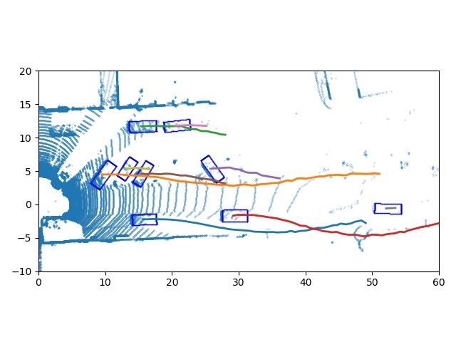
2                                                  IEEE ROBOTICS AND AUTOMATION LETTERS. PREPRINT VERSION. ACCEPTED FEBRUARY, 2021

association relationship of the proposals in a batch of point       networks are used widely in forecasting tasks like trajectory
clouds as input, to replace the appearance features by merging      prediction [6] [7].
the neighbor location and detection embeddings.                        Social LSTM [7] was proposed to learn the movements of
   For multiple object tracking (MOT) tasks, data association,      the general human and predict the trajectories of multiple
which is the process of associating the same object in different    pedestrians, and sequential data are used to provide short-
frames, is one of the key technologies. In contrast to the          term and long-term information. ReSeg [8] was proposed for
methods described in Fig. 1(a) [3], [4], [1], and (b) [2], we       semantic segmentation in different scenarios as an RNN-based
want to propose an end-to-end network (Fig. 1(c)), which can        network. This kind of usage is more like an alternative to
get straight to the track ID of each object without the data        Convolutional Neural Networks (CNNs), which shows that
association step.                                                   RNN models have the ability to learn the dependencies
   In this paper, we propose an end-to-end tracking with            between time connection data. Wang et al. [9] proposed a
detection neural network, DiTNet, which directly outputs the        Bayesian and conditional random field-based framework in
3D bounding box with the track ID of each object in the             the Spatio-temporal map to solve the data association problem
Spatio-temporal world. DiTNet takes as input the raw point          between frames. A Spatio-temporal LSTM [10] which uses
cloud batch (numbers of adjacent point cloud frames), and           sequential data as input was introduced to save the long-term
outputs each object’s detection bounding box in the frames          context information. Structural-RNN [11] combines the high-
and track ID in the batch. There are two critical issues in the     level Spatio-temporal graphs with RNNs, which reconstructs
network. One is that the number of trajectories is not constant,    the factors in Spatio-temporal graph to achieve a rich RNN
which means we could have 0 to L trajectories. The other is         mixture.
that the order of trajectories is not required to be fixed, which      Though the features of the same object are always changing
means the track identity is unordered. The same object only         over time in 3D point clouds, the related location information
needs to be classified into one trajectory, no matter what the      over the whole sequence can also help to rearrange the track
track ID is. These two issues are especially prominent during       IDs of the detections. Thus, in our network, the long-term
network training. In our approach, we set a max number of           temporal and spatial features are consolidated to finish the
trajectories to solve the first issue, and apply the Hungarian      data association end-to-end.
algorithm [5] to efficiently assign the predicted trajectories
with label trajectories for the second. Note that the Hungarian
algorithm is only used while training, and it is not necessary      B. 3D Object Detection and Tracking
in the inference processing. The contributions of this work are        In existing 3D object detection solutions, 3D point cloud-
listed as follows:                                                  based networks can predict more accurate locations and the
   • We propose a novel detection arrangement method in the         bounding boxes of objects compared to 2D images. Networks
      Spatio-temporal map to learn the correlation relationship     like those in [12] and [13] use PointNet++ [14] as the 3D
      of objects in a batch of frames as input.                     backbone to learn the 3D features from dense to sparse. And
   • We propose an instance-based network, which uses novel         other networks [15] still preserve the image-based 2D CNN
      grouping and feature extraction layers to learn the cor-      to compose the large-scale features by scattering the learned
      relation location information and instance features in the    features from pillars or voxels to the Bird’s-eye-view map.
      spatial and temporal feature modules.                            For multi-object tracking problems, most of the current
   • We propose a real end-to-end detection network to out-         approaches focus on the data association problem. The Kalman
      put the objects’ boxes and track IDs directly, without        Filter [3] [4] and Gaussian [16] processes are all famous as the
      the usage of non-maximum suppression (NMS) and the            conventional methods for position prediction and association
      Hungarian algorithm.                                          matrix generation, and convolutional Siamese networks [17]
   • The sequence of the point cloud input can be used              [18] are also used widely for association similarity compu-
      to improve the performance of detection and tracking.         tation. Once the cost matrix of all objects is obtained, the
      Our approach achieves competitive performance over the        data association problem can also be seen as an optimization
      state-of-the-art methods on the KITTI benchmark.              problem. Thus, the Hungarian algorithm [3] can be applied to
   The remainder of this letter is organized as follows. Sec-       solve it. Matching Net [19] [20] can find the corresponding
tion II reviews the related work. Section III describes the         pairs in adjacent frames and generate the trajectories. Multi-
framework and components of DiTNet in detail. Section IV            scan methods, which take as input a sequence of data rather
presents the experimental results and discussions. Conclusions      than two single adjacent frames, have proposed to use a
and future work are given in the last section.                      neural network to learn the optimization solutions to find the
                                                                    optimal trajectory assignment [21] [19]. Meanwhile single-
                                                                    scan methods only take as input two adjacent frames and
                   II. RELATED WORK
                                                                    associate the objects in these two frames [22] [2], by predicting
A. Time-Related Networks                                            the association matrix or the movement of each object to find
   In time series-related tasks, different kinds of network         the best association relationship. AB3DMOT [1] and DEEP
architectures focus on the importance of temporal relations in      SORT [4], which are two baseline tracking-by-detection ap-
a batch of data, such as Recently Recurrent Neural Networks         proaches, use rich texture features of each object as attributes
(RNN) and Long Short Term Memory (LSTM). Time-related               of the objects and the Kalman Filter and Hungarian algorithm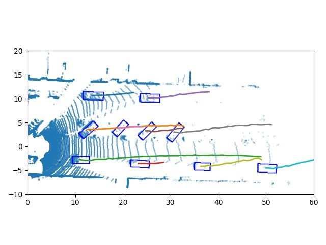
WANG et al.: DITNET 3
Input Detection Module Tracking Module Training Loss Module Output
3Dbackbone
Assigned
Track ID
Track ID
Track ID
Temporal Feature Module
ID
Point Cloud Batch
Head
Spatial Feature Module
Scatter to BEV
Assignment
Layer
2Dbackbone
Track ID Loss
Refined Box
Refinement
Refine Loss
RPN Head
Det Loss
Head
Box
ROI Box
GT Track ID GT Box
Fig. 2: The overall network architecture. The detection module takes the continuous point cloud batch as input and generates
the ROIs with high-level features. Then the tracking module uses them to get the refined boxes with the track ID. The training
loss module only works during the training to calculate the ground-truth ID assignment matrix and the training loss.
as post-process association methods to finish the real-time 2D multi-scale backbone. Finally, the detection head uses two
tracking. convolutional layers which have a 1 × 1 kernel to predicts the
3D bounding boxes with their class for objects in each pillar
III. OUR APPROACH position. Axis-aligned NMS is performed at inference time.
A. The Overall Architecture The detection module can be replaced by any other 3D
object detector, as long as its output includes the detection
The overall architecture of our DiTNet is shown in Fig.
results with their high-level features. The critical consideration
2. The network is composed of three main parts: the detec-
in choosing the best detector backbone is to balance speed
tion module, Spatio-temporal tracking module, and training
and detection performance. Whether the input of the detector
loss module. The detection module outputs the positions
is a 3D point cloud or 2D image is not the key factor in our
and bounding boxes of the ROIs from the raw point cloud
tracking task, because if the input is raw point clouds which
data batch. The embeddings of the ROIs and the boxes are
have minor texture information of the objects, the Spatio-
combined as the detections and passed to the tracking module
temporal module will learn the relative position information
(Sec III-B). The tracking module can output the unique track
of all neighboring objects to find the correct corresponding
ID of each object in a batch of adjacent frames, and then
relationship. How to choose the detection score threshold of
an easy post-processing algorithm is used to connect the track
NMS is one of the crucial problems of most tracking-by-
ID in the whole sequence. The architecture of Spatio-temporal
detection methods, because the tracking task is more sensitive
tracking module is inspired by the arrangement of detections
to false-positive detections than the detection task. Other
in the Spatio-temporal world (Sec III-C). The training loss
methods choose to use a higher score threshold to filter the
module in the blue block in Fig. 2 is time-consuming but only
unreliable detections, but our proposed detection module uses
works while training, which means that, although the network
a small threshold to ensure as many detections as possible
needs a longer time for training, it is efficient enough for real-
will be included for the next tracking process. The high-level
time inference (Sec III-D).
features of the detections then contribute to the following
tracking module.
B. Detection Module
The detection module is proposed to generate the 3D C. Tracking Module
ROIs of each possible object with its learnable features. As From the detection module, we can get: the object detec-
introduced in [23], there are four main modules in current tions’ absolute global location {Lti = (xti , yti , zti )}Ni=1
t
, where x,
state-of-the-art detectors: the 3D backbone, 2D backbone, ROI y, and z are the 3D global position of the objects at time t,
head, and dense detection head. Our detection module makes and Nt means there are at most Nt objects at each time; the
reference to PointPillars [15], which consists of three submod- objects’ detection score {Sti }Ni=1
t
, where S ∈ [0, 1], S ∈ R; and
ules: a 3D pillar feature net, 2D encoder-decoder backbone, the middle embeddings of each object from the 2D backbone
and RPN detection head. Firstly, we discretize the raw 3D in the detection module {Cit }Ni=1 t
, where each feature has K-
points into evenly spaced grids in the ground plane, which dim channels. We use a multi-scan point cloud batch as input,
are called pillars. Each pillar is fed separately into the voxel which is obtained by using a sliding window to crop batches
feature encoding (VFE) network to extract the 3D embeddings of data. Let T denote the window size, and we can obtain the
inside every pillar, which can be scattered back to the 2D BEV object detections in this time window: {Dti }i∈[1,Nt ],t∈[1,T ] . The
pseudo-image using their position index. A 2D CNN backbone detections are rearranged in the Spatio-temporal world with
is then applied to generate multi-scale high-level features from their global xyz location in a single frame, and also with their
the pseudo-image. We use C to denote the output features, moment of appearance. A t axis is proposed in Spatio-temporal
which is concatenated from different upsampling layers in the world to store the time information.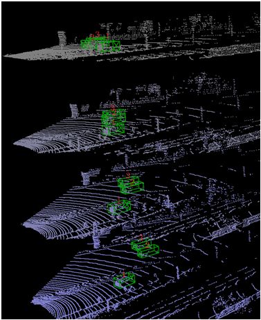
4                                                     IEEE ROBOTICS AND AUTOMATION LETTERS. PREPRINT VERSION. ACCEPTED FEBRUARY, 2021

    The detections from the detection module have four main                In the global feature module, only the grouping method
properties: (1) The detections are unordered, which means               is different from the local feature module. It will choose all
they can be arranged in different orders by their positions             detections in the same time frame, except the target detection
and features. In other words, our network should be able to             itself, as the grouped detections, and the MLPs are used for
learn the order-invariant features of all detections. (2) All of        the weighted relative embeddings learning.
the various detections in a single frame must have their own               2) Temporal feature extraction module: Compared with the
unique track IDs. (3) The detections are not isolated within            spatial feature extraction module, the temporal feature module
the environment; in other words, the neighborhoods of each              mainly learns the relative spatial features in the different time
detection can provide feature information while learning. (4)           frames.
The tracking results should have invariance under trajectory               Take Fig. 3 (a) as an example. The object with track ID 1
transformation. For example, theoretically, the tracking results        is the most leftward detection in all time frames, object 2 is
should be the same when the trajectories appear in different            in the middle, and object 3 is the most rightward detection.
places, without considering the environment’s influence, as             Thus the spatial features from the spatial feature extraction
long as all detections have the same relative position of all           module will be clustered into three groups, for objects 1, 2,
pairs in the whole sequence. Another example is that the                and 3 respectively. We can use the temporal feature module
time interval ∆t in a sequence is not the key factor because            to find the objects in different frames with the most similar
       |Lt −Lt+1 |
vti = i ∆ti        , where Lti and Lt+1i    ∈ R3 are the absolute       embeddings. And in Fig. 3 (b), we can find that there are two
location, is the speed of objects. And the speed of different           false-positive detections in time frame 2 and time frame 3.
objects or the same objects at different times is not a constant        The temporal feature module is proposed to learn the relative
in a real environment.                                                  location displacement of each object from others in different
    To fit these special properties in the tracking task, we discard    time frames. Thus object 4 will be tracked successfully due
all absolute global locations or features in the Spatio-temporal        to the smooth trajectory.
feature module, while using the relative location information              As shown in Fig. 3 (d), we predict the temporal features
and relative features to represent the relative relationship of         frame by frame. All detections learn the embeddings from
objects to objects. dk in Fig. 3 means the relative features: for       the detections in different time frames. For each object in
                                                                                       t                                  t
target detection D ∈ RK , grouped neighbor detections Dg =              time t0 , {Di0 }, i ∈ [1, Nt ], the objects Gi j ,t j 6= t0 , i ∈ [1, Nt ]
{Dg i }, Dg ∈ RK , i ∈ [1, Nn ], dk = D − Dg = {D − Dg i }, and i ∈     will be grouped. For grouped objects in each time frames
[1, Nn ].                                                               ({t j = 1, 2, ..., T,t j 6= t0 }), the learning function is the same
    The tracking module consists of three main parts: a spatial         as the frame global feature extraction module in Eq. 1. And
feature extraction module, temporal feature extraction module,          after obtaining each set ofgrouped features, the mean pooling
and track head module.                                                  method is used to merge all features in this batch of data. The
    1) Spatial feature extraction module: The spatial feature           temporal feature network can be described by:
extraction module consists of a local feature extraction module
                                                                                       ft (D, G) = MEAN( f (W · (pDt , Gt ))).                (2)
and a frame global feature extraction module, as shown in Fig.                                      t=1,...,T
3 (c). The local feature module learns the relative features from
                                                                           The MaxPool can be explained as finding the most similar
the nearest S neighbor detections, and the frame global module
                                                                        object, and the MeanPool helps to merge all information of
learns the relative features from all detections in the same time
                                                                        each trajectory in the whole time batch.
frame.
             t                                                             3) Track Head: As shown in Fig. 3 (e), the track head
    Take Di00 as the target detection for example. In the local
                                                                        module consists of two heads: a track ID head and box
feature extraction module, the grouping layer chooses the
                           t                                            refinement head. Two separate conv. layers with 1 × 1 kernels
nearest objects G = {Di0 }, where i 6= i0 , the number of grouped
                                                                        are used in these two heads for the predicted track ID and
objects is less than the maximum grouping number Ns , and
    t      t                                                            the refined box detection. The problem is how to assign the
||Li0 − Li00 ||2 ≤ dLmax .
                                                                        predicted bounding boxes to the ground-truth, and how to
    Given an unordered detection set {D1 , D2 , ..., DNt } with their
                                                                        assign the unordered track IDs to the ground-truth IDs. The
locations and embeddings Di = (Li ,Ci ), where Li ∈ Rd ,Ci ∈
                                                                        solution to these problems is described in the training and
RK , the local feature module defines a set function f : X → R:
                                                                        testing section as follows.
        f ({D1 , D2 , ..., DNt }) = MAX (γ(W · (G − Di ))),      (1)
                                 i=1,...,Nt
                                                                        D. Training and Testing
where γ is multi-layer perceptron (MLP) networks, and W is
                                                                          The one-hot track ID generator is proposed to generate the
the weight of each relative embeddings. W is calculated by
                                                                        one-hot track IDs, and in the training process of DiTNet,
the distance between each grouped detection and the target
                                                                        an ID assignment layer is used to reorder the predicted one-
detection and the detection score of the target detection. For
                                                                        hot track IDs with the ground-truth IDs, for subsequent loss
normalization, the distance weight is calculated by:
                                                                        computation. In the process of testing, DiTNet takes as input
          Wi j = Ws ·WdL = Si j · exp(−α · ||Li − G j ||),              the raw point cloud batch and directly outputs the track ID
                                                                        with the detection bounding box of each object without the
where α is a parameter which is set to 10 in our experiment.            Hungarian algorithm or other data association methods.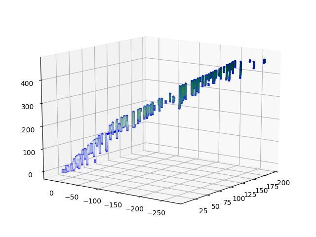
WANG et al.: DITNET 5
(a) (c) Frame Global Feature (d) (e)
Group Layer
Grouped t = T - 1
N×N×dK
t=3 (128, 128, 256)
MaxPool
(128, 128) 7
N×128
1 3 2
N×128
t=T
T×N×N×dK
T×N×7
Group Layer
T×N×256
MaxPool
Shared mlp
t=2 1 3 2
…
MeanPool
N×128
Shared mlp
T×N×(128+256)
…
…
…
…
t = 11 3 2
T×N×128
T×N×K
…
Grouped t = 1
N×N×dK
MaxPool
N×128
(b)
4
N×128
t=3
T×N×S×dK
Group Layer
t=2
-1 L+1
T×N×128
T×N×(L + 1)
MaxPool
Shared mlp
…
…
4
t=2 -1 … …
N×128
t=1
4
t=1 (64, 128, 128)
Local Feature Temporal Feature
Fig. 3: Two schematics of the common detection distribution and details of the tracking module in DiTNet. (a) An example of
spatial feature-based object detection distribution. (b) An example of temporal feature-based object detection distribution. (c)
Spatial feature extraction module, which is concatenated by frame global feature extraction module and local feature extraction
module. (d) Temporal feature extraction module. (e) Tracking head, which outputs the refined bounding boxes with their track
ID. The dots in (a-b) are detections, and red dashed lines are ground-truth trajectories. The red blocks in (c–e) are MLPs with
1 × 1 kernels, and the number means the number of kernels.
One-hot track identity generator: Firstly, a softmax func- the predicted unordered trajectories with the ground-truth
tion is applied for each object’s track ID. Then we find the trajectory to get the ordered trajectories. Then the network loss
largest track ID probabilities one by one, and make sure each can be calculated. Note again that the Hungarian algorithm is
object only has one track ID and each chosen ID is unique in only proposed to assign the predicted track identity with the
a single time frame. ground-truth identity for network training. This step does not
ID Assignment Layer: Due to the randomness of the track exist in the inference process.
ID assigned to each trajectory, we cannot directly calculate the Post-processing: During the inference process, the network
loss between the predicted tracking trajectory and the ground- predicts the track IDs in each batch. And by moving the afore-
truth trajectory. Therefore, for the training process, we design mentioned sliding window step by step, for each predicted
a track ID assignment layer to find the matchings between track ID, the algorithm will check whether the objects with
the predicted trajectories and the ground-truth trajectories. this ID have existed in the past trajectories. If yes, then the
This layer takes as input the predicted trajectories as well as fresh detection will be added to the existing trajectory, and if
the ground-truth trajectories, and assigns the most matched the brand new track ID has not appeared before, then a new
ground-truth track ID to the predicted one. trajectory will be added to the full trajectory list.
We employ the IoU as the cost metric to measure how well Loss Function: Our loss consists of detection loss and
a pair of trajectories matches. It calculates the ratio of the tracking loss, and tracking loss consists of a binary cross
number of overlapping points to the total number of points in entropy loss Lmask , a softmax IoU (SIoU) loss LSIoU , a
a pair. Since the number of predicted trajectories varies, it is softmax cross entropy loss for each trajectory Luniqe for track
reasonable to set L ≥ L̄, where L is the number of predicted uniqueness, and a triplet loss Ltri :
trajectories and L̄ is the number of ground-truth trajectories.
The size of the output of the track ID module is T × Nt × L = Ldet + Ltra + Lre f ine (4)
(L + 1), where Nt is the maximum number of detections and
1 is the dustbin for the false track ID. Let {Tri , Tr j } denote a Ltra = Lmask + α · LsIoU + β · Luniqe + γ · Ltri , (5)
pair of trajectories, and I ∈ RL×L̄ denote the reordering matrix.
After discarding the dustbin of the false track ID channel, we where α, β , and γ are weighting parameters, which are set to
can get Ci, j ∈ RL×L̄ as the cost for the matching, where L 0.1, 1, and 1.
is the predicted track ID and L̄ is the ground-truth ID. The The detection ROI loss Ldet and the box refinement loss
assignment problem can be formulated as a bipartite matching Lre f ine are calculated the same as in the setting in [15]. Lmask
problem: is computed from the score tracking score of each point:
L L̄ Lmask = −s · log(ŝ) − (1 − s) · log(1 − ŝ), (6)
argmin ∑ ∑ Ii, jCi, j
I i=1 j=1 where s ∈ {0, 1} is the ground-truth, 1 represents that the
subject to: 0 ≤ i ≤ L, 0 ≤ j ≤ L̄, (3) object detection is negative and 0 otherwise, and ŝ is the
L predicted dustbin score of each object detection. With the
Ii, j ∈ {0, 1}, ∑ Ii, j = 1, for ∀ j. associated tracking trajectories, we calculate the SIoU with:
i=1
In this paper, we use the Hungarian algorithm [5] to solve 1 L ∑Nn=1 fnl · gln
LSIoU = 1 − ∑ , (7)
this problem. With the matching matrix I, we can associate L l=1 ∑Nn=1 fnl + ∑Nn=1 gln − ∑Nn=1 fnl · gln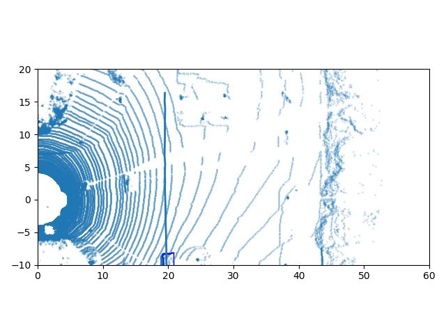
6 IEEE ROBOTICS AND AUTOMATION LETTERS. PREPRINT VERSION. ACCEPTED FEBRUARY, 2021
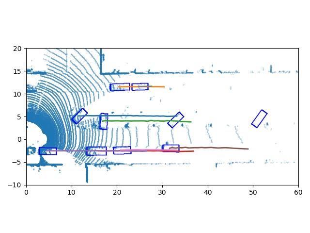
ST-Map with trajectories Time = 30 frame Time = 60 frame Time = 90 frame
Fig. 4: The qualitative results. Top row is the visualization of tracking results of sequence 0 in the KITTI test dataset, and
bottom row is tracking results of sequence 1. The leftmost column is the detection results and trajectories in Spatio-temporal
world, the detections are green points and trajectories are blue lines. The three rightmost columns are the trajectories on the
BEV of the LiDAR data at different time stamps.
where fnl ∈ [0, 1] is the probability for point n to have the number of detections in each time frame to Nt = 90 to include
trajectory l, which is obtained by applying a softmax function all detection ROIs in the detection module of DiTNet. We
on the trajectory class prediction for point n, gln ∈ {0, 1} set the maximum number of trajectories in each time stamp
represents the ground-truth, and N is the number of points. to Mmax = 60. The size of the track ID label of each point is
Focal loss [24] is applied in the trajectories’ uniqueness loss: N × (Mmax + 1). Its first channel belongs to negative detections
and redundancies. The window size is set to 4 and the step
Lunique = mask · (−α(1 − p)γ log(p)), (8) size is set to 1 in our experiments for on-line inference.
where p is the object’s positive probability in each trajectory, Multiple Object Tracking Accuracy (MOTA), Multiple Ob-
mask ∈ {0, 1} is the ground-truth of each trajectory, and α = ject Tracking Precision (MOTP), Mostly Tracked (MT), Most-
0.25, γ = 2. The mask will be 0 if the trajectory does not exist ly Lost (ML), ID Switches (IDS) and fragmentation (FRAG)
in this point cloud batch. This loss only considers the positive from the CLEAR MOT metrics[46] are used for evaluating the
trajectories, and it helps that each trajectory will only appear detection and tracking accuracy.
once in each time frame. As our task resembles the instance
segmentation and re-ID, we borrow the triplet loss [25] for our B. Ablation Study and Comparative Results
task. It encourages the embeddings from the same track to stay We conduct ablation studies on two key factors: the length
as close as possible, while different tracks are separated as far of the input point cloud batch, and the score threshold of the
as possible. Specifically, we choose the batch hard triplet loss detection module for tracking. We also present two compara-
in [25]. tive experiments in this section. First of all, we compare our
DiTNet to AB3DMOT [1], RANSAC200, RANSAC1000, and
IV. EXPERIMENTS PointTrackNet [2]. RANSAC [26], which can be seen as one
of the tracking-by-detection methods, is used here to generate
A. Dataset and Evaluation Metrics the trajectories in the Spatio-temporal map. It connects the
We train and evaluate our model on two datasets. One is detections as a conventional trajectory fitting method. In our
the object tracking benchmark dataset from KITTI [34]. The comparative experiments, we split our pre-trained end-to-end
other is the simulation dataset generated from CARLA [35]. network into a detection module and a tracking module. Only
Our approach is trained on the CARLA dataset and the the detection results are fed into RANSAC as the input. Thus
first half of 21 sequences from KITTI which have ground- it makes sense to compare the tracking-by-detection RANSAC
truth labels, and is evaluated on CARLA and the last half of with our end-to-end DiTNet when the detection results are the
the 21 sequences from the KITTI dataset. We uploaded our same. RANSAC200 means it iterates 200 times in the fitting
test results of the 29 test sequences on KITTI that need to be process in each Spatio-temporal map, while RANSAC1000
evaluated online. Since the KITTI dataset mainly uses vehicles means it iterates 1000 times. In our experiments, the trajec-
as the validation type, we track the Car and Van categories tories are all assumed to be conics in the x-t, y-t, and z-t
only in that dataset. And in the CARLA dataset, we set the planes. When we have an estimated conic trajectory, "inliers"
number of pedestrians to 30 and the number of vehicles to mean the objects which have less than the threshold distance
20. Considering misdetections like false-positives, we set the from the trajectory at that time. The inlier threshold is set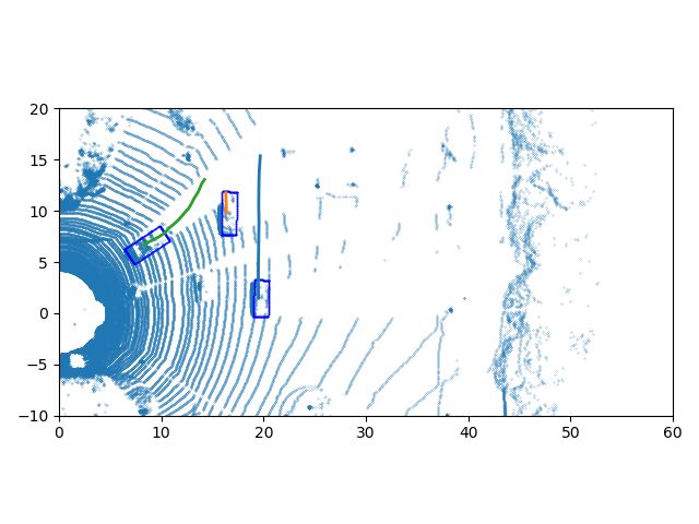
WANG et al.: DITNET                                                                                                                                       7

 TABLE I: C OMPARATIVE R ESULTS OF E VALUATION M ETRICS WITH D IFFERENT D ETECTION S CORE T HRESHOLDS FOR
   D IFFERENT T RACKERS IN THE KITTI VALIDATION DATASET. T HE B OLD F ONT H IGHLIGHTS THE B EST R ESULTS .
                                                                           Car
                                        Det Score Threshold = 0.2                                              Det Score Threshold = 0.6
         Method
                          MOTA↑     MOTP↑     MT↑        ML↓        IDS↓         FRAG↓      MOTA↑          MOTP↑        MT↑    ML↓         IDS↓   FRAG↓
    RANSAC200 [26]         0.5077    0.867    0.2836     0.3085       78          441            0.578     0.8714    0.3351   0.2251       121     436
    RANSAC1000 [26]        0.7404   0.8677    0.6099     0.0762      212          626           0.7806     0.8712    0.6667    0.062       287     647
     AB3DMOT [1]           0.6977   0.8653    0.7553     0.0319        8          168           0.7431     0.8678    0.7322   0.0319         6     264
    DiTNet (length=2)      0.6743   0.8682    0.7438     0.0306       82          134           0.7203     0.8762     0.732   0.0502        47     131
    DiTNet (length=3)      0.7855   0.8654    0.7942     0.0354       57          153           0.7928      0.877    0.7462   0.0543        34     142
    DiTNet (length=4)      0.7865   0.8680    0.8103     0.0393       22          105           0.8108     0.8783    0.7935   0.0421        20     120
    DiTNet (length=5)       0.786   0.8683    0.8081     0.0397       23          112           0.8012     0.8791    0.7813   0.0421        20     123
                                                                     Pedestrian
                                        Det Score Threshold = 0.2                                              Det Score Threshold = 0.6
         Method
                          MOTA↑     MOTP↑     MT↑        ML↓        IDS↓         FRAG↓      MOTA↑          MOTP↑        MT↑    ML↓         IDS↓   FRAG↓
    RANSAC200 [26]         0.4101   0.6709    0.2178     0.1188      551          1041          0.4521      0.67     0.2375    0.099       631    1087
    RANSAC1000 [26]        0.4155   0.6713    0.3168      0.099      659          1134          0.4833     0.6705    0.3168   0.0891       637    1114
     AB3DMOT [1]           0.4799   0.6699    0.4356     0.0693       83           435          0.5446     0.6699    0.4059   0.0693        72     451
    DiTNet (length=2)      0.4236   0.6823    0.4105     0.0553      153           403          0.5674     0.6834    0.4246   0.0653       124    587
    DiTNet (length=3)      0.4879   0.6822    0.4253     0.0521      148           412          0.5982     0.6823    0.4272   0.0615       122     564
    DiTNet (length=4)      0.5841   0.6823    0.4554     0.0495      104           384          0.6104     0.6836    0.4455   0.0594       102     401
    DiTNet (length=5)      0.5786   0.6816    0.4521     0.0495      102           386          0.6124     0.6842    0.4416   0.0594        97     412

                TABLE II: C OMPARATIVE R ESULTS OF E VALUATION M ETRICS ON THE KITTI T EST DATASET.
                      Methods        MOTA↑      MOTP↑        MT↑           ML↓           IDS↓      FRAG↓     Runtime↓         Environment
               SRK-ODESA [27]        90.03%     84.32%      82.62%     2.31%               90        501        0.4s              GPU
                 JRMOT [28]          85.70%     85.48%      71.85%      4.00%              98        372       0.07s       4 cores @ 2.5 Ghz
               MOTSFusion [29]       84.83%     85.21%      73.08%      2.77%             275        759       0.44s              GPU
                 mmMOT [30]          84.77%     85.21%      73.23%      2.77%            284        753        0.02s        GPU @ 2.5 Ghz
                mono3DT [31]         84.52%     85.64%      73.38%      2.77%             377        847       0.03s        GPU @ 2.5 Ghz
                AB3DMOT [1]          83.84%     85.24%      66.92%     11.38%               9        224      0.0047s      1 core @ 2.5 Ghz
             3D-CNN/PMBM [32]        80.39%     81.26%      62.77%     6.15%              121        613       0.01s       1 core @ 3.0 Ghz
                FANTrack [19]        77.72%     82.33%      62.62%      8.77%             150        812       0.04s      8 cores @ >3.5 Ghz
             Complexer-YOLO [22]     75.70%     78.46%      58.00%      5.08%            1186       2092       0.01s        GPU @ 3.5 Ghz
                mbodSSP* [33]        72.69%     78.75%      48.77%      8.77%             114        858       0.01s       1 core @ 2.7 Ghz
                 Point3DT [2]        68.24%     76.57%      60.62%     12.31%             111        725       0.05s      1 core @ >3.5 Ghz
                 DP-MCF [21]         38.33%     78.41%      18.00%     36.15%            2716       3225       0.01s       1 core @ 2.5 Ghz
                DiTNet (Ours)        84.62%     84.18%      74.15%     12.92%              19        196       0.01s      1 core @ >3.5 Ghz

to 1 meter, considering the detection error. The window size                     evaluation metrics on the KITTI test dataset. It reveals DiT-
and step size in the Spatio-temporal map generation process                      Net’s competitive performance over the other state-of-the-art
are also set to be same as our method. The number of                             methods. The running time of 0.01 seconds makes it possible
iterations depends on the complexity of the detection result.                    for real-time tracking tasks.
More iterations are needed to find the suitable trajectories in
much denser environments. In the KITTI validation dataset,                       C. Qualitative Results
when the number of iterations is larger than 1000, the tracking
                                                                                    Fig. 4 shows the qualitative results on the KITTI test dataset.
results show very limited changes. The ablation studies’ results
                                                                                 This part of the dataset has no publicly available labels and
are also compared with these methods.
                                                                                 our network still has good results. We choose to visualize the
   Tab. I shows the comparative results and ablation studies                     tracking results of sequence 0 and 1. The trajectories on the
of the evaluation metrics with a different detection score                       BEV of the LiDAR data at three different time stamps are
threshold for different trackers. The length means the length                    shown in the three rightmost columns in the figure. We find
of the point cloud batch. We can find that our proposed DitNet                   only one ID switch, which is circled in red in sequence 0. In
outperforms others on MOTA by remarkable margins, which                          the 29 sequences of the KITTI test dataset, our network only
means the overall tracking performance is much better than                       has 19 ID switches and 196 trajectory fragmentations in total.
that of the others. Besides this, we choose the ROI detection
results as the detection for other tracking-by-detection meth-                                             V. CONCLUSIONS
ods, and our DiTNet can refine the detections, which makes
                                                                                    We proposed here a real end-to-end tracking with detection
the performance on MOTP better than that of other methods.
                                                                                 network, which can directly output the detection box and
  Next we compare our tracking results with the publicly                         track identity of each object without data association. Our
available state-of-the-art approaches from the KITTI tracking                    approach outperforms others on the KITTI benchmark on both
benchmark. Tab. II shows the comparative results of the                          the MOTP and IDS. In the future, we will try to fuse the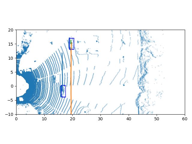
8                                                           IEEE ROBOTICS AND AUTOMATION LETTERS. PREPRINT VERSION. ACCEPTED FEBRUARY, 2021

camera with LiDAR to achieve more complex textures of each                      [19] E. Baser, V. Balasubramanian, P. Bhattacharyya, and K. Czarnecki,
object to improve the tracking performance.                                          “Fantrack: 3d multi-object tracking with feature association network,”
                                                                                     in 2019 IEEE Intelligent Vehicles Symposium (IV). IEEE, 2019, pp.
                                                                                     1426–1433.
                             R EFERENCES                                        [20] L. Bertinetto, J. Valmadre, J. F. Henriques, A. Vedaldi, and P. H. Torr,
                                                                                     “Fully-convolutional siamese networks for object tracking,” in European
 [1] X. Weng, J. Wang, D. Held, and K. Kitani, “3d multi-object tracking: A          conference on computer vision, 2016, pp. 850–865.
     baseline and new evaluation metrics,” arXiv preprint arXiv:1907.03961,     [21] H. Pirsiavash, D. Ramanan, and C. C. Fowlkes, “Globally-optimal
     2020.                                                                           greedy algorithms for tracking a variable number of objects,” in CVPR
 [2] S. Wang, Y. Sun, C. Liu, and M. Liu, “Pointtracknet: An end-to-end              2011. IEEE, 2011, pp. 1201–1208.
     network for 3-d object detection and tracking from point clouds,” 2020.    [22] M. Simon, K. Amende, A. Kraus, J. Honer, T. Samann, H. Kaulbersch,
 [3] A. Bewley, Z. Ge, L. Ott, F. Ramos, and B. Upcroft, “Simple online              S. Milz, and H. Michael Gross, “Complexer-yolo: Real-time 3d object
     and realtime tracking,” in 2016 IEEE International Conference on Image          detection and tracking on semantic point clouds,” in Proceedings of
     Processing (ICIP). IEEE, 2016, pp. 3464–3468.                                   the IEEE Conference on Computer Vision and Pattern Recognition
 [4] N. Wojke, A. Bewley, and D. Paulus, “Simple online and realtime                 Workshops, 2019, pp. 0–0.
     tracking with a deep association metric,” in 2017 IEEE International       [23] O. D. Team, “Openpcdet: An open-source toolbox for 3d object detection
     Conference on Image Processing (ICIP). IEEE, 2017, pp. 3645–3649.               from point clouds,” https://github.com/open-mmlab/OpenPCDet, 2020.
 [5] H. W. Kuhn, “The hungarian method for the assignment problem,” Naval       [24] P. Yun, L. Tai, Y. Wang, C. Liu, and M. Liu, “Focal loss in 3d object
     research logistics quarterly, vol. 2, no. 1-2, pp. 83–97, 1955.                 detection,” IEEE Robotics and Automation Letters, vol. 4, no. 2, pp.
 [6] K. Saleh, M. Hossny, and S. Nahavandi, “Long-term recurrent predictive          1263–1270, 2019.
     model for intent prediction of pedestrians via inverse reinforcement       [25] A. Hermans, L. Beyer, and B. Leibe, “In defense of the triplet loss for
     learning,” in 2018 Digital Image Computing: Techniques and Applica-             person re-identification,” arXiv preprint arXiv:1703.07737, 2017.
     tions (DICTA). IEEE, 2018, pp. 1–8.                                        [26] M. A. Fischler and R. C. Bolles, “Random sample consensus: a paradigm
 [7] A. Alahi, K. Goel, V. Ramanathan, A. Robicquet, L. Fei-Fei, and                 for model fitting with applications to image analysis and automated
     S. Savarese, “Social lstm: Human trajectory prediction in crowded               cartography,” Communications of the ACM, vol. 24, no. 6, pp. 381–395,
     spaces,” in Proceedings of the IEEE conference on computer vision and           1981.
     pattern recognition, 2016, pp. 961–971.                                    [27] D. Mykheievskyi, D. Borysenko, and V. Porokhonskyy, “Learning local
 [8] F. Visin, M. Ciccone, A. Romero, K. Kastner, K. Cho, Y. Bengio,                 feature descriptors for multiple object tracking,” in Proceedings of the
     M. Matteucci, and A. Courville, “Reseg: A recurrent neural network-             Asian Conference on Computer Vision, 2020.
     based model for semantic segmentation,” in Proceedings of the IEEE         [28] A. Shenoi, M. Patel, J. Gwak, P. Goebel, A. Sadeghian, H. Rezatofighi,
     Conference on Computer Vision and Pattern Recognition Workshops,                R. Martin-Martin, and S. Savarese, “Jrmot: A real-time 3d multi-object
     2016, pp. 41–48.                                                                tracker and a new large-scale dataset,” arXiv preprint arXiv:2002.08397,
 [9] S. Wang, H. Huang, and M. Liu, “Simultaneous clustering classification          2020.
     and tracking on point clouds using bayesian filter,” in 2017 IEEE          [29] J. Luiten, T. Fischer, and B. Leibe, “Track to reconstruct and reconstruct
     International Conference on Robotics and Biomimetics (ROBIO). IEEE,             to track,” IEEE Robotics and Automation Letters, 2020.
     2017, pp. 2521–2526.                                                       [30] W. Zhang, H. Zhou, S. Sun, Z. Wang, J. Shi, and C. C. Loy, “Ro-
[10] J. Liu, A. Shahroudy, D. Xu, and G. Wang, “Spatio-temporal lstm with            bust multi-modality multi-object tracking,” in Proceedings of the IEEE
     trust gates for 3d human action recognition,” in European conference            International Conference on Computer Vision, 2019, pp. 2365–2374.
     on computer vision. Springer, 2016, pp. 816–833.                           [31] H.-N. Hu, Q.-Z. Cai, D. Wang, J. Lin, M. Sun, P. Krahenbuhl, T. Darrell,
[11] A. Jain, A. R. Zamir, S. Savarese, and A. Saxena, “Structural-rnn:              and F. Yu, “Joint monocular 3d vehicle detection and tracking,” in
     Deep learning on spatio-temporal graphs,” in Proceedings of the ieee            Proceedings of the IEEE international conference on computer vision,
     conference on computer vision and pattern recognition, 2016, pp. 5308–          2019, pp. 5390–5399.
     5317.                                                                      [32] S. Scheidegger, J. Benjaminsson, E. Rosenberg, A. Krishnan, and
[12] S. Shi, X. Wang, and H. Li, “Pointrcnn: 3d object proposal generation           K. Granström, “Mono-camera 3d multi-object tracking using deep learn-
     and detection from point cloud,” in Proceedings of the IEEE Conference          ing detections and pmbm filtering,” in 2018 IEEE Intelligent Vehicles
     on Computer Vision and Pattern Recognition, 2019, pp. 770–779.                  Symposium (IV). IEEE, 2018, pp. 433–440.
[13] Z. Ding, X. Han, and M. Niethammer, “Votenet: a deep learning label        [33] P. Lenz, A. Geiger, and R. Urtasun, “Followme: Efficient online min-cost
     fusion method for multi-atlas segmentation,” in International Conference        flow tracking with bounded memory and computation,” in Proceedings
     on Medical Image Computing and Computer-Assisted Intervention.                  of the IEEE International Conference on Computer Vision, 2015, pp.
     Springer, 2019, pp. 202–210.                                                    4364–4372.
                                                                                [34] A. Geiger, P. Lenz, and R. Urtasun, “Are we ready for autonomous
[14] C. R. Qi, L. Yi, H. Su, and L. J. Guibas, “Pointnet++: Deep hierarchical
                                                                                     driving? the kitti vision benchmark suite,” in 2012 IEEE Conference on
     feature learning on point sets in a metric space,” in Advances in neural
                                                                                     Computer Vision and Pattern Recognition. IEEE, 2012, pp. 3354–3361.
     information processing systems, 2017, pp. 5099–5108.
                                                                                [35] A. Dosovitskiy, G. Ros, F. Codevilla, A. Lopez, and V. Koltun, “Carla:
[15] A. H. Lang, S. Vora, H. Caesar, L. Zhou, J. Yang, and O. Beijbom,
                                                                                     An open urban driving simulator,” arXiv preprint arXiv:1711.03938,
     “Pointpillars: Fast encoders for object detection from point clouds,” in
                                                                                     2017.
     Proceedings of the IEEE Conference on Computer Vision and Pattern
     Recognition, 2019, pp. 12 697–12 705.
[16] T. Hirscher, A. Scheel, S. Reuter, and K. Dietmayer, “Multiple extended
     object tracking using gaussian processes,” in 2016 19th International
     Conference on Information Fusion (FUSION). IEEE, 2016, pp. 868–
     875.
[17] J. Zbontar and Y. LeCun, “Computing the stereo matching cost with a
     convolutional neural network,” in Proceedings of the IEEE conference
     on computer vision and pattern recognition, 2015, pp. 1592–1599.
[18] W. Luo, A. G. Schwing, and R. Urtasun, “Efficient deep learning for
     stereo matching,” in Proceedings of the IEEE Conference on Computer
     Vision and Pattern Recognition, 2016, pp. 5695–5703.
You can also read