Grasshopper optimization algorithm optimized multistage controller for automatic generation control of a power system with FACTS devices
←
→
Page content transcription
If your browser does not render page correctly, please read the page content below
Nayak et al. Protection and Control of Modern Power Systems                    (2021) 6:8
https://doi.org/10.1186/s41601-021-00187-x
                                                                                                                          Protection and Control of
                                                                                                                            Modern Power Systems

 ORIGINAL RESEARCH                                                                                                                                   Open Access

Grasshopper optimization algorithm
optimized multistage controller for
automatic generation control of a power
system with FACTS devices
Pratap Chabdra Nayak, Ramesh Chandra Prusty*                               and Sidhartha Panda

  Abstract
  This paper uses a Grasshopper Optimization Algorithm (GOA) optimized PDF plus (1 + PI) controller for Automatic
  generation control (AGC) of a power system with Flexible AC Transmission system (FACTS) devices. Three differently
  rated reheat turbine operated thermal units with appropriate generation rate constraint (GRC) are considered along
  with different FACTS devices. A new multistage controller design structure of a PDF plus (1 + PI) is introduced in the
  FACTS empowered power system for AGC while the controller gains are tuned by the GOA. The superiority of the
  proposed algorithm over the Genetic Algorithm (GA) and Particle Swarm Optimization (PSO) algorithms is
  demonstrated. The dynamic responses of GOA optimized PDF plus (1 + PI) are compared with PIDF, PID and PI
  controllers on the same system. It is demonstrated that GOA optimized PDF plus (1 + PI) controller provides
  optimum responses in terms of settling time and peak deviations compared to other controllers. In addition, a
  GOA-tuned PDF plus (1 + PI) controller with Interline Power Flow Controller (IPFC) exhibits optimal results compared
  to other FACTS devices. The sturdiness of the projected controller is validated using sensitivity analysis with
  numerous load patterns and a wide variation of parameterization. To further validate the real-time feasibility of the
  proposed method, experiments using OPAL-RT OP5700 RCP/HIL and FPGA based real-time simulations are carried
  out.
  Keywords: Automatic generation control, FACTS devices, Multistage controller, Grasshopper optimization algorithm

1 Introduction                                                                          power network is to limit the transient frequency
In a multi-area power system, qualitative, reliable, se-                                deviation, inter-line power exchange, and to reduce
cure, stable and economic action of the system requires                                 steady-state errors to zero [2]. An epidemic power sys-
stable frequency and power transmission across a tie-                                   tem is an amalgamation of a large electrical network and
line preserved at their nominal values. Symmetry in a                                   within the network, each area is known as a control area
power system will be maintained when proper coordin-                                    and the areas are braided with one another over various
ation is established between power requirement and                                      tie-lines. In an electric network, the system operation
generation. Two control mechanisms are assigned, i.e.,                                  must be proficient in establishing equilibrium in ex-
reactive power control (Automatic voltage regulator                                     change power across a tie-line and in securing frequency
AVR) which maintains voltage profile and real power                                     stabilization. Many nonlinear loads (equipped with
control through the AGC system [1] for frequency                                        power semiconductor devices) interlinked with a dis-
stabilization. The responsibility of AGC in a multi-area                                persed power system network introduce large transient
                                                                                        disturbances in the electrical network resulting in a mis-
* Correspondence: ramesh.prusty82@gmail.com                                             match between generation and demand. Thus, the
Department of Electrical Engineering, VSSUT, Burla, Odisha 768018, India

                                        © The Author(s). 2021 Open Access This article is licensed under a Creative Commons Attribution 4.0 International License,
                                        which permits use, sharing, adaptation, distribution and reproduction in any medium or format, as long as you give
                                        appropriate credit to the original author(s) and the source, provide a link to the Creative Commons licence, and indicate if
                                        changes were made. The images or other third party material in this article are included in the article's Creative Commons
                                        licence, unless indicated otherwise in a credit line to the material. If material is not included in the article's Creative Commons
                                        licence and your intended use is not permitted by statutory regulation or exceeds the permitted use, you will need to obtain
                                        permission directly from the copyright holder. To view a copy of this licence, visit http://creativecommons.org/licenses/by/4.0/.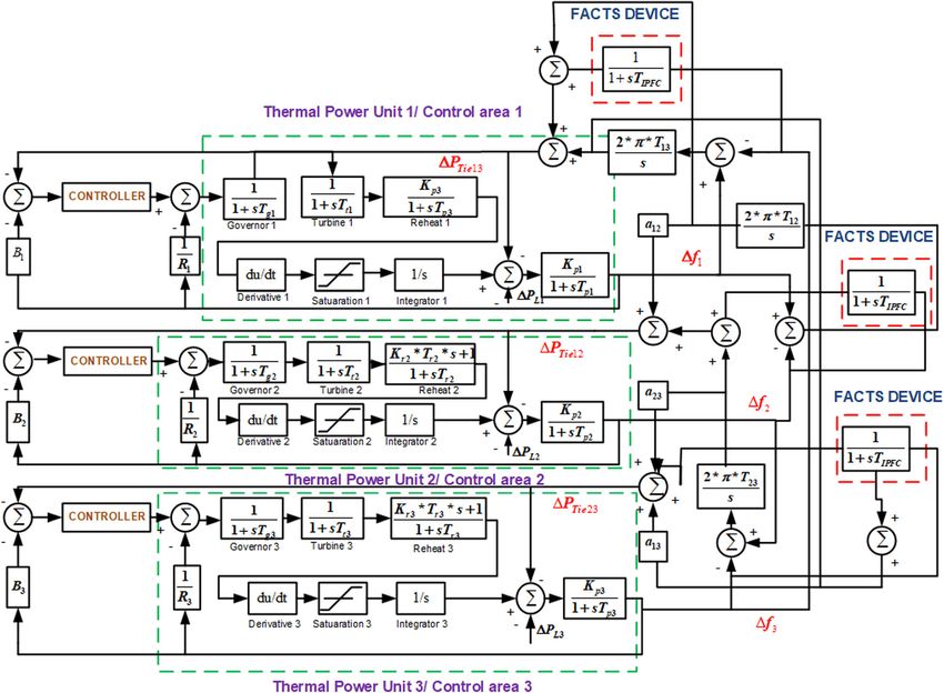
Nayak et al. Protection and Control of Modern Power Systems   (2021) 6:8                                             Page 2 of 15

automatic control system has to be upgraded with mod-                method is exactly appropriate for all types of problems
ern techniques for stable, reliable and economical oper-             and there is scope for improvement by proposing new
ation [3].                                                           techniques/controller.
   In a modern power system, the rapid development                     Conventional tuning methods are based on a single
of power semiconductor devices gives opportunities to                objective trial and error type. This often takes up more
design fast-acting FACTS devices [4]. Power system                   time and most often produces substandard results. Ref-
stability has reached a new height and power flow                    erence [13] used hybrid DEPS, while [15] adopted DE
control becomes more flexible using modern FACTS                     and [18] used PSO for optimization. However, these
devices. Much recent research explores the effect of                 classical methods have the problem of getting trapped in
FACTS devices in AGC, e.g., Thyristor controlled                     local optima. Many methods have been used to try to
phase shifter (TCPS), Static Synchronous Series                      address these problems, e.g., firefly algorithm (FA) [12],
Compensator (SSSC) and various combinations                          Symbiotic Organisms Search SOS [16], BAT [19], Grey
equipped in series with a tie-line integrated with                   Wolf Optimization GWO [20], and Cuckoo Search (CS)
SMES have been implemented to normalize frequency                    [23]. The efficacy of the sine cosine algorithm in the
deviations under various restraints of a 2-area system               AGC system with FACTS devices was explored in [24],
[5]. Steadiness of frequency oscillation is achieved by              while better dynamic performance using GWO was ob-
a fractional order based SSSC controller in [6] while                tained in [21] and in [22], the primacy of GOA with a 2-
TCPS-SMES was implemented in DFIG-based wind                         stage controller was explored.
farm integrated power systems in [7] [8, 9]. used                      The GOA approach uses a node finite input for excita-
redox flow batteries interlinked with IPFC and a Thy-                tion and it has a simple user interface. It was extensively
ristor Controlled Series Capacitor (TCSC), while [10,                used in [25] for tuning controller gains. In this paper,
11] used TCSC for stability control in IPFC, and an                  the GOA algorithm is embedded with a PDF plus (1 +
SMES-UPFC combination was used in a 2-area 6-unit                    PI) controller in the AGC of a 3-area thermal power net-
system in [12].                                                      work for the escalation of gains in the presence of con-
   Many have introduced various modern control strat-                trasting FACTS devices.
egies including modified structures of the classical con-              Sensitivity investigation observed the robustness of the
trollers of I, PI and PID in the AGC system. The                     most favorable controller gains [21–23]. Similar investi-
dynamic responses of classical controllers in AGC have               gation has been carried out for the optimum controller
been evaluated in [13, 14], while [15] proposed parallel             in the presence of FACTS devices in AGC, and the most
2DOF-PID for LFC in a power system with GDB. The                     convenient objective function for optimum controller
fuzzy-PID controller was preferred to establish cohesion             and FACTS devices is investigated.
in power system dynamic behavior in [16–18], while cas-
                                                                       The main objectives of the present research work are:
caded PD-PID and PI-PD controllers were used in [19,
20] because of their adequate results, simplicity, reliabil-
                                                                        Introduction of GOA for extensive modulation of
ity and performance. A 2DOF controller was imple-
                                                                           controller gains of an AGC in a 3-area thermal
mented in [19] to minimize the steady-state error and to
                                                                           power network.
establish stability in the system, while [21, 22] satisfied a
                                                                          Introduction of a metamorphic PDF plus (1 + PI)
system necessity by introducing a metamorphic modern
PDF+(1 + PI) controller which helped in developing the                     controller in the AGC, consisting of a filter with PD
responses of transient and steady-state error to diminish                  and (1 + PI). The time-variant responses are equated
with different dynamic responses with various parts.                       with PI, PID and PIDF controllers for efficacy
   In this paper, a PDF+(1 + PI) controller consisting of a                measurement.
PD controller with filter and a (1 + PI) controller con-                  Comparison of the dynamic performance of a 3-area
nected in series, is examined with the influence of FACT                   thermal power network with FACTS devices along
S devices in an AGC multi-area thermal power system.                       with a metamorphic PDF plus (1 + PI) controller.
Contemporary memetic nature-inspired innovations                          To compare the performance of GOA with PSO and
have been evolved to carry out a comprehensive search.                     GA for a controller design problem for the same test
The efficacy of the memetic algorithm can be assessed                      system.
by evidence that they emulate the finest outcome glo-                     Performance comparison of IPFC with SSSC, TCPS
bally, specifically the excerpt of the competent in organic                and TCSC for frequency regulation.
systems that have emerged by instinctive assortment                       Sensitivity analysis of a 3-area thermal power net-
over decades. From the literature survey, it is evident                    work with the best location of IPFC and optimum
that many optimization techniques/ controllers have                        controller gains, by changing the percentage of step
been applied to various problems but no meta-heuristic                     load perturbation (SLP) and system parameters.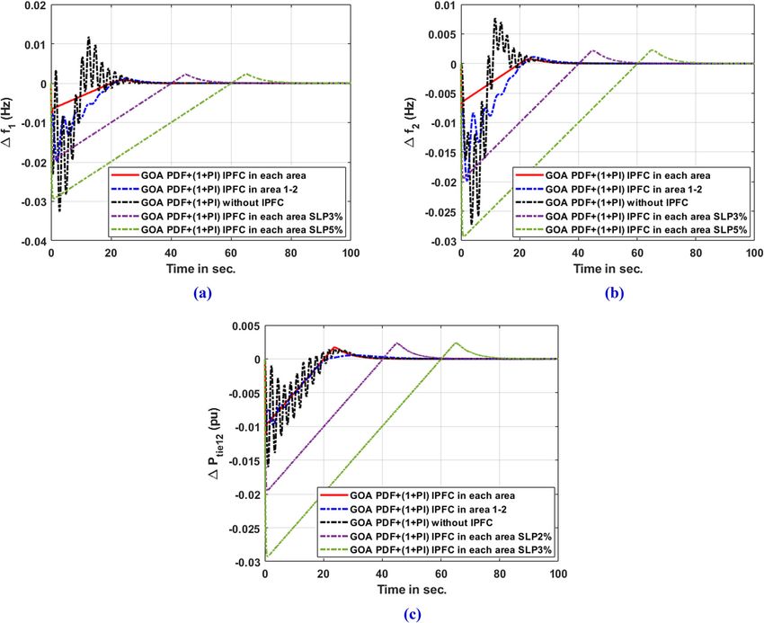
Nayak et al. Protection and Control of Modern Power Systems   (2021) 6:8                                                       Page 3 of 15

   Validation of simulation results by an OPAL-RT                   proposed control model of the 3-area thermal network
     OP5700 real-time simulator.                                     is presented in Fig. 1 and the relevant parameters are
                                                                     shown. The different possible combinations of various
                                                                     controllers with several FACT devices are optimized
2 Model investigated                                                 with GA, PSO and GOA for comparison with the pro-
A 3-area thermal power network is proposed for ana-                  posed strategy.
lysis, where the size of area1 is 2000 MW, area2 is 6000
MW and area3 is 1200 MW. In this network model,                      2.1 Objective function
nonlinearity constraints are extensively introduced by               The objective functions, IAE, ITAE, ISE and ITSE are
the implementation of GRC which is set at 3% with a re-              examined for obtaining optimum results in frequency
heat turbine in each control section. The nominal pa-                stabilization and tie-line power control. The correspond-
rameters of the model are given in Table 7 in Appendix.              ing objective function accepts ΔFi and ΔPtie i-j as inputs
Several classic PI, PID and PDF controllers with the                 and actions are taken to minimize them to zero by tuned
metamorphic PDF plus (1 + PI) controller are considered              controller gains.
individually for study. Dynamic investigations of the 3-               Mathematical expressions for the objective functions
area thermal power network with the independent influ-               are:
ence of SSSC, TCSC, TCPS and IPFC are carried out in
                                                                                         Z   T
the presence of the GOA technique-tuned PDF plus                                                                       2
(1 + PI) controller. The dynamic performance in each                       J 1 ¼ ISE ¼            ðΔF i Þ2 þ ΔP tiei − j dt            ð1Þ
                                                                                         0
control area is estimated by setting SLP at 1%. The

 Fig. 1 Simulation prototype of a reheat turbine fitted thermal network with 1% SLP and 3% GRC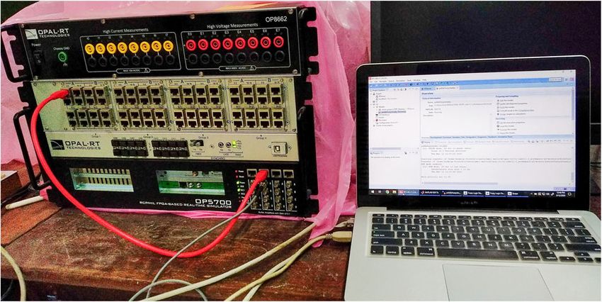
Nayak et al. Protection and Control of Modern Power Systems        (2021) 6:8                                            Page 4 of 15

                                                                          conditions and the minimization of steady-state error
                                                                          in dynamic analysis of any system is demonstrated in
                                                                          many studies. By the presence of integral gain, rapid-
                                                                          ity in minimization of steady-state error is achieved
                                                                          and system stability is reduced in the transient condi-
                                                                          tion. For better response in the transient condition,
                                                                          the integral parameter must not be engaged in action
 Fig. 2 Structure of PDF plus (1 + PI) controller                         all along the transient period. With the enhancement
                                                                          of prominent dynamic response of the system some
                    Z          T                         2            refitted control structures have evolved which are
    J 2 ¼ ITSE ¼                    ðΔ F i Þ2 þ ΔP tiei − j tdt    ð2Þ
                           0
                   Z       T
    J 3 ¼ IAE ¼                jΔ F i j þ ΔPtiei − j  dt         ð3Þ
                       0
                       Z       T
    J 4 ¼ ITAE ¼                    jΔ F i j þ ΔPtiei − j  tdt   ð4Þ
                           0

  where ΔFi is the frequency fluctuation in the ith area
and ΔPtie i − j is the tie-line power fluctuation in the ith
and jth area.

2.2 Models of FACTS devices
For smooth management of tie-line power control
using fine adjustment of the relative phase angle be-
tween the two control areas is feasible using TCPS.
This helps in the settlement of frequency oscillations
as well as inter-exchange of active power across the
tie-line. Transient stability can be achieved by coun-
teracting the oscillations with well-managed control-
ler damping on the disrupted system. SSSC
incorporates a voltage with adjustable magnitude in
the quadrature with the current equivalent to a con-
trollable inductive or capacitive reactance to influ-
ence the tie-line power flow. The transfer function
models of TCPS and SSSC are adapted from [5, 7].
IPFC provides reactive series compensation effi-
ciently in inductive or capacitive fashion so that the
tie-line power flow can be effectively managed by
the IPFC through the injection of an accurate series
reactive compensating voltage [8, 9]. The control
prototype of the IPFC has been acquired from [8].
TCSC can be employed in multi-transmission lines
to effectively introduce series compensation for dy-
namic change in transmission line reactance. The
transfer function of TCSC is presented in [10, 11]
while the criteria of TCPS, SSSC, TCSC and IPFC
are taken from [5, 7–11, 21]. As shown in Fig. 1,
IPFC is in series with the three control areas.

2.3 Proposed PDF plus (1 + PI) controller
Having a simple system interface makes the PID con-
troller the most encouraging tool for many studies.
The PID controller offers efficacy in most transient                        Fig. 3 The flowchart representation of GOA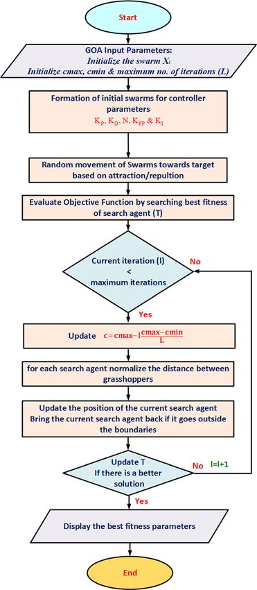
Nayak et al. Protection and Control of Modern Power Systems (2021) 6:8 Page 5 of 15
Table 1 Statistical analysis of different agents for GOA, PSO and GA optimized PDF plus (1+ PI) controllers
Functions Test Functions Parameters GOA PSO GA
F1 Shifted Sphere Function Average 1.6219X1056 8.931X1066 9.2656 X10²¹
Pn
f 1 ðxÞ ¼ x 2i Standard Deviation 1.6266X10 57
7.0111X10 68
4.1437 X10²²
i¼1
Minimum 0.1088X10³ 0.0059X10³ 0.0021 X10³
68 66
Maximum 1.8291X10 9.468X10 1.8531 X10²³
F2 Shifted Schwefel’s Function Average 3.7673 X1067 13.045 X10¹¹ 1.4177 X1024
Pn Q
f 2 ðxÞ ¼ jx i j þ ni¼1 jx i j Standard Deviation 3.7688 X10 68
11.366X10 12
1.428 X1025
2
i¼1
Minimum 0.0062 X10³ 0.0379 X10³ 0.0023 X10³
69 13
Maximum 3.8265 X10 13.415 X10 1.4319 X1024
F3 Shifted Rosenbrock’s Average 2.7399 X1032 12.121 X10⁹ 4.3317 X10¹⁹
Function 33 11
Pn Standard Deviation 1.0523 X10 11.598 X10 3.9854 X10²⁰
f 3 ðxÞ ¼ ð½x i þ 0:5Þ2
i¼1 Minimum 0.0161 X10³ 4.686 X10² 0.0082 X10³
33 13
Maximum 4.0777 X10 10.032 X10 4.3987 X10¹⁹
F4 Shifted Rastrigin’s Function Average 5.2988 X1044 6.8166 X1038 2.2347 X1027
Pn
f 4 ðxÞ ¼ ½x 2i þ 10 cosð2πx i Þ þ 10 Standard Deviation 2.9021 X10 45
7.0025 X10 39
1.4921 X1028
i¼1
Minimum 0.0063 X10³ 1.792 X10² 0.0076 X10³
46 41
Maximum 1.5896 X10 9.568 X10 2.4682 X1027
F5 Shifted Schwefel’s Problem with Noise in Fitness Average 2.2974 X1034 5.6982 X1034 3.8751 X10²²
f5(x) = max {|xi|, 1 ≤ i ≤ n} 35 38
Standard Deviation 2.2798 X10 6.2784 X10 2.9852 X10²³
Minimum 0.0009 X10³ 0.0561 X10³ 0.0023 X10³
36 36
Maximum 2.2799 X10 5.5862 X10 4.0012X10²²
F6 Schwefel’s Problem with Global Optimum on Bounds Average 3.0414 X1030 2.1187 X1042 1.8955 X1043
Pn
2
f 6 ðxÞ ¼ ½100ðx iþ1 − x 2i Þ þ ðx i − 1Þ2 Standard Deviation 2.5276 X10 31
1.5182 X10 44
1.9865 X1044
i¼1
Minimum 0.0015 X10³ 0.172 X10² 0.0089 X10³
32 45
Maximum 2.4682 X10 2.930 X10 2.2219 X1043
F7 Shifted Rotated Griewank’s Function Average 3.4099 X1033 11.530 X1035 7.6482 X1034
Pn
f 7 ðxÞ ¼ ix 4i þ random½0; 1 Standard Deviation 2.4053 X10 34
13.028 X10 36
5.6214 X1035
i¼1
Minimum 0.0008 X10³ 1.406 X10² 0.0019 X10³
35 38
Maximum 1.8920 X10 11.022 X10 4.5875 X1034
F8 Shifted Rotated Ackley’s Function with Global Optimum on Bounds Average 5.0129 X1032 6.321 X1031 8.8626 X1029
P
n pffiffiffiffiffiffi
f 8 ðxÞ ¼ − x i sinð jx i jÞ Standard Deviation 2.2418 X10 33
5.4213X10 32
4.5897 X1030
i¼1
Minimum 0.0018 X10³ 2.1235X10³ 0.0062 X10³
34 33
Maximum 1.0026 X10 8.082X10 6.9871 X1029
proficient in transient stability establishment. This is The mathematical expression of the PDF plus (1 + PI)
accomplished by a metamorphic PDF plus (1 + PI) controller is given as:
controller, which minimizes the error in the steady-
state and at the same time manages speed and system Ns KI
Tf PDFþð1þPI Þ ¼ KP þ KD 1 þ K PP þ
stability. The controller consists of two stages, the 1st N þs s
stage is a PD controller with filter and the 2nd stage ð5Þ
is a 1 plus PI controller. To perform the corrective
action ACE is accepted as input by the PDF control- As shown, there are different elements of the PDF plus
ler and the output of this is endorsed by the PI con- (1 + PI) controller, i.e., KP, KI, KD, KPP and N. The Area
troller. The structure of the proposed controller is control error (ACE) is input to the controller and the
shown in Fig. 2. output signal will be the input for the power network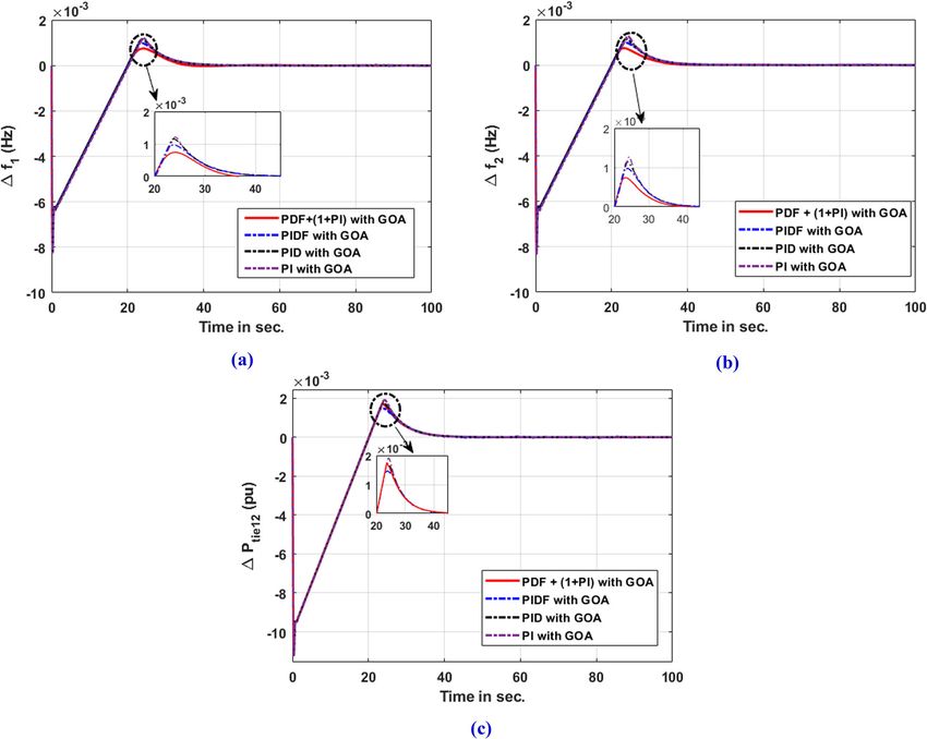
Nayak et al. Protection and Control of Modern Power Systems   (2021) 6:8                                           Page 6 of 15

                                                                                                X
                                                                                                n
                                                                           ACE i ¼ βi Δ F i þ         ΔPtiei − j           ð6Þ
                                                                                                j¼1
                                                                                                j≠i

                                                                     3 Grasshopper optimization algorithm
                                                                     The Grasshopper Optimization Algorithm (GOA) is a
                                                                     contemporary multifaceted anatomical method pro-
                                                                     posed in [25]. The GOA approach is based on the life
 Fig. 4 Study of the different objective functions with GOA
                                                                     cycle of the grasshopper, which consists of three
                                                                     stages of egg, nymph and adult going through a
                                                                     process called metamorphosis. Grasshoppers migrate
with the addition of changes in tie-line power and                   from egg to nymph as sliding cylinders, and then
frequency.                                                           when they migrate from nymph to metamorphosis,
  ACE is the difference between the actual power gener-              they damage crops. This nature is mathematically
ation and the scheduled generation with the influence of             modeled to form an anatomical optimization tech-
frequency bias, and is given as:                                     nique named GOA. It has two aspects: first, during
                                                                     the investigation it searches for members, and then it

 Fig. 5 Dynamic responses of different GOA optimized controllers with 1% SLP and IPFC device in each area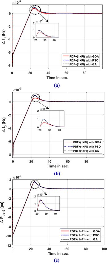
Nayak et al. Protection and Control of Modern Power Systems        (2021) 6:8                                                         Page 7 of 15

Table 2 Peak deviation and settling time for effectiveness measurement of PDF plus (1 + PI) controller
Element      Peak Overshoot (+)                               Peak Undershoot (−)                                Settling Time in seconds
             PI        PID        PIDF      PDF + (1 + PI) PI           PID        PIDF        PDF + (1 + PI) PI       PID    PIDF PDF + (1 + PI)
Δf1 (Hz)     0.001205 0.001184 0.000963 0.000740              0.008266 0.007891 0.007613 0.007415                44.65 41.25 38.34 34.22
Δf2 (Hz)     0.001269 0.001163 0.000976 0.000735              0.008362 0.008184 0.007771 0.007567                43.71 41.95 39.39 37.07
Δf3 (Hz)     0.001139 0.001131 0.000977 0.000551              0.008305 0.008102 0.007551 0.006845                44.50 42.64 40.68 38.12
ΔPtie1–2(pu) 0.001873 0.001718 0.001434 0.001674              0.011169 0.010894 0.009867 0.008423                52.58 45.31 43.22 42.68
ΔPtie2–3(pu) 0.001875 0.001693 0.001548 0.001458              0.011421 0.011228 0.011205 0.010127                54.88 42.39 41.17 37.84
ΔPtie3–1(pu) 0.001751 0.001697 0.001676 0.001467              0.011308 0.011235 0.011218 0.010113                49.81 45.45 42.22 40.96

moves nearby in the exploitation. This ensures the
goal is accomplished logically.
  The congregate behavior of ‘Grasshoppers’ is precisely                        sðr Þ ¼ fe − r=l − e − r                                     ð10Þ
articulated as follows:                                                   where f is the potential of likeness and l is the detach-
    X m ¼ S m þ Gm þ Am                                           ð7Þ     ment of likeness force.
                                                                           The G factor in (8) is evaluated as:
where Xm is the location of the mth Grasshopper, Sm is
the correlation, Gm is the gravitational strength on the                        Gi ¼ − g ebg                                                 ð11Þ
mth Grasshopper, and Am is the wind in abeyance. The                      where g is the gravitational force constant and ebg is a
equation can be upgraded to allow for arbitrary nature                    unity vector focused on along the earth’s center.
as:                                                                        The A factor in (8) is evaluated as:
                                                                                Am ¼ uebw                                                    ð12Þ
    X m ¼ r 1 S m þ r 2 Gm þ r 3 Am                               ð8Þ
                                                                          where u is a constant drift and c ew is a unity vector for
where r1, r2, and r3 are arbitrary coefficients, and                      the wind course.
                                                                            Replacing S, G, and A in (8) yields:
             X
             k                                                                            X
                                                                                          k
                                                                                                                 xn − xm
    Sm ¼           sðd mn Þdd
                            mn                                    ð9Þ           Xm ¼             sðjxn − xm jÞ           − g ebg þ uebw      ð13Þ
                                                                                                                   d mn
           n¼1                                                                            n¼1
           n≠m                                                                            n≠m

where dmn is the gap among the mth and nth Grasshop-                      where n is the number of grasshoppers.
pers, dmn = | xn– xm |, s is the function of collective
                   xn − xm
forces, and dd mn ¼ dmn is a unit vector from the m to
                                                    th
  th
n Grasshoppers.
   The s function for the collective forces (dislike and
like) is given as:

 Fig. 6 Study of the objective function with PDF plus (1 + PI)                Fig. 7 Convergence curves for GA, PSO & GOA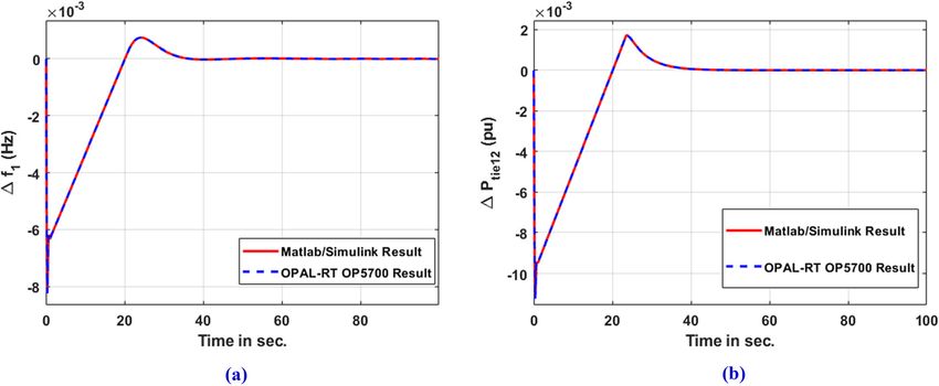
Nayak et al. Protection and Control of Modern Power Systems   (2021) 6:8                                                    Page 8 of 15

                                                                       For optimization on the global horizon, (13) is altered
                                                                     as:
                                                                                   0                                          1
                                                                                    B X                                         C
                                                                                    B k      ubd − lbd  d
                                                                                                                    d  xn − xm C
                                                                                                                                C
                                                                           X m d ¼ cB
                                                                                    B      c          s   x n − x m
                                                                                                                                    c
                                                                                                                                C þ Td
                                                                                    @n ¼ 1       2                        d mn A

                                                                                       n≠m
                                                                                                                                   ð14Þ

                                                                     where ubd is the Dth aspect upper bound, lbd is the Dth
                                                                     aspect lower bound, T cd is the Dth aspect of the objective
                                                                     bound, and c is a declining factor to minimize the com-
                                                                     fort zone, dislike zone and like zone. Based on current
                                                                     place, GOA unceasingly updates the location of an in-
                                                                     vestigation agent, global optimum and the location of all
                                                                     other investigation agents.
                                                                       The comfort zone reduces, and coefficient c is pro-
                                                                     portional to the number of iterations and is evalu-
                                                                     ated as:

                                                                                           c max − c min
                                                                           c ¼ c max − l                                           ð15Þ
                                                                                                 L
                                                                        where cmax is the max value, cmin is the min value, l
                                                                     indicates the current iteration, and L is the number of
                                                                     iterations.
                                                                        GOA is initiated by forming a collection of random
                                                                     results, and searching representatives upgrade their
                                                                     location at each iteration by (13). At the termination
                                                                     of every iteration, the finest marked location is
                                                                     upgraded. In addition, factor c is evaluated using (14)
                                                                     and the linearization of gaps among grasshoppers is
                                                                     carried out in every repetition. Adaptation is made it-
                                                                     eratively until the final criterion is matched, and the
                                                                     global optimum comes out as the best approximation
                                                                     returned finally by the position and fitness of the best
                                                                     target. The flowchart of the GOA technique is given
                                                                     in Fig. 3.

                                                                     3.1 Statistical analysis of GOA
                                                                     Statistical analysis of the proposed PDF plus (1 + PI) con-
                                                                     troller with different algorithms of GOA, PSO and GA opti-
                                                                     mized for standard deviation, min, max and average values
                                                                     of fitness function is presented in Table 1. It is clear from
                                                                     Table 1 that functions F5, F6, F7, and F8 for GOA give
 Fig. 8 Dynamic responses of different techniques of GOA,            good average results, and function F6 with SD = 2.5276
 PSO and GA optimized with PDF plus (1 + PI), with 1% SLP            X1031 provides the best results in all respects out of the 23
 and IPFC device in each area                                        predefined objective functions. Functions F2 with SD =
                                                                     1.428 X1025 and F5 with SD = 6.2784 X1038 provide the
                                                                     best results in the cases of GA and PSO, respectively.

                                                                     4 Results and discussions
                                                                     The study is carried out using MATLAB R2019a,
                                                                     while the multi-thermal power system model is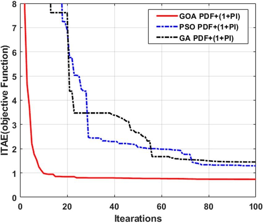
Nayak et al. Protection and Control of Modern Power Systems (2021) 6:8 Page 9 of 15
Table 3 Peak deviation and settling time for effectiveness measurement of GOA with PDF plus (1 + PI) controller
Element Peak Overshoot (+) Peak Undershoot (−) Settling Time in seconds
GA PSO GOA GA PSO GOA GA PSO GOA
Δf1 (Hz) 0.000983 0.000949 0.000740 0.008227 0.007562 0.007415 46.13 42.89 34.22
Δf2 (Hz) 0.001013 0.000948 0.000735 0.008228 0.007643 0.007567 47.16 43.91 37.07
Δf3 (Hz) 0.000974 0.000912 0.000551 0.008225 0.007998 0.006845 46.37 42.61 38.12
ΔPtie1–2(pu) 0.001832 0.001698 0.001674 0.011228 0.010935 0.008423 44.67 43.57 42.68
ΔPtie2–3(pu) 0.001536 0.001572 0.001458 0.011231 0.010564 0.010127 42.16 40.28 37.84
ΔPtie3–1(pu) 0.001547 0.001422 0.001467 0.011159 0.011032 0.010113 46.02 41.53 40.96
developed in SIMULINK with the reheat turbine, shown in Fig. 4. Compared to PIDF, PID and PI, the
GRC and PDF plus (1 + PI) controller. The GOA, improvements in the ITAE error with the proposed GOA
PSO and GA programs are in script-file and function- tuned PDF plus (1 + PI) controller are 3.43%, 5.38% and
file of MATLAB R2019a. The exploration is carried 7.86%, respectively.
by 100 agents and 100 iterations are reserved for en- The dynamic behavior of the power system fre-
tire investigations. The efficacy authentication of the quency and tie-line power for each controller is
different objective functions is carried out by setting compared in Fig. 5(a)-(c). Performance indices such
each control area with 1% SLP at t = 0 s. as the maximum overshoot and undershoot, and set-
tling time of the dynamic responses, are given in
4.1 Effectiveness of PDF plus (1 + PI) controller Table 2. From Fig. 5 and Table 2, it is evident that
In this segment, the 3-area thermal power network the proposed PDF plus (1 + PI) controller is better
fitted with reheat turbine, GRC and IPFC in each than the classical PI, PID and PIDF controllers with
control area is examined by various controllers such lowest settling time of 34.22 s (Δf1) and peak
as PI, PID, PIDF and PDF plus (1 + PI) optimized by fluctuations.
the GOA technique. The obtained controller gains are
as follows:
PI controller in each area: 4.2 Effectiveness of the GOA algorithm
In this section, the effectiveness of the structural
K P1 ¼ 0:0169; K P2 ¼ 0:3187; K P3 ¼ 1:9829; algorithm-based GOA method is verified with the pro-
K I1 ¼ 1:8142; K I2 ¼ 1:9035; K I3 ¼ 1:6172; posed PDF plus (1 + PI) controller. The thermal power
system network is fitted with the IPFC controller in each
PID controller in each area:
area, while GRC is set at 3% and all SLP are fixed to 1%.
K P1 ¼ − 0:0619; K P2 ¼ − 0:0232; K P3 ¼ 1:9963; Figure 6 shows the fitness of the best objective function al-
K D1 ¼ − 0:0032; K D2 ¼ 0:0027; K D3 ¼ 0:1427; gorithm, with GOA optimized PDF plus (1 + PI) controller
K I1 ¼ 1:9541; K I2 ¼ 1:9375; K I3 ¼ 1:6514; with ITAE value 0.422 × 10⁻² having the lowest among
the entire statistical data.
PIDF controller in each area: Compared to PSO and GA, the improvements in the
K P1 ¼ 0:4724; K P2 ¼ 0:7055; K P3 ¼ 0:7323; ITAE error with the proposed GOA tuned PDF plus (1 +
K D1 ¼ 0:0512; K D2 ¼ 0:0138; K D3 ¼ 0:2113; PI) controller are 12.26% and 17.57%, respectively. Figure 7
K I1 ¼ 1:8212; K I2 ¼ 1:9375; K I3 ¼ 1:614; provides complete information regarding the convergence
N 1 ¼ 33:8127; N 2 ¼ 74:9604; N 3 ¼ 2:5760; of fitness function (ITAE) with PDF plus (1 + PI) control-
ler for GOA, PSO and GA techniques. The dynamic
PDF plus (1 + PI) controller in each area: frequency stabilization and tie-line power flow is shown in
Fig. 8(a)-(c) and Table 3. The GOA method shows
K P1 ¼ − 1:9255; K P2 ¼ 1:8659; K P3 ¼ 1:9547;
performance superior to that of GA and PSO methods
K PP1 ¼ − 1:8694; K PP2 ¼ 0:3766; K PP3 ¼ 0:1075;
with the same setting and strategy.
K D1 ¼ 0:0071; K D2 ¼ 0:1114; K D3 ¼ 0:0045;
K I1 ¼ − 1:9161; K I2 ¼ 1:9219; K I3 ¼ 1:9372;
N 1 ¼ 48:9384; N 2 ¼ 0:0720; N 3 ¼ 48:1291;
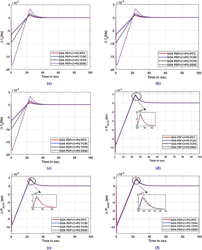
4.3 Effectiveness of several FACTS devices
The comparative analysis of different objective functions In this section, four FACTS devices, i.e., TCPS, SSSC,
with the various controllers with the GOA algorithm is TCSC, and IPFC are tested in the 3-area thermal power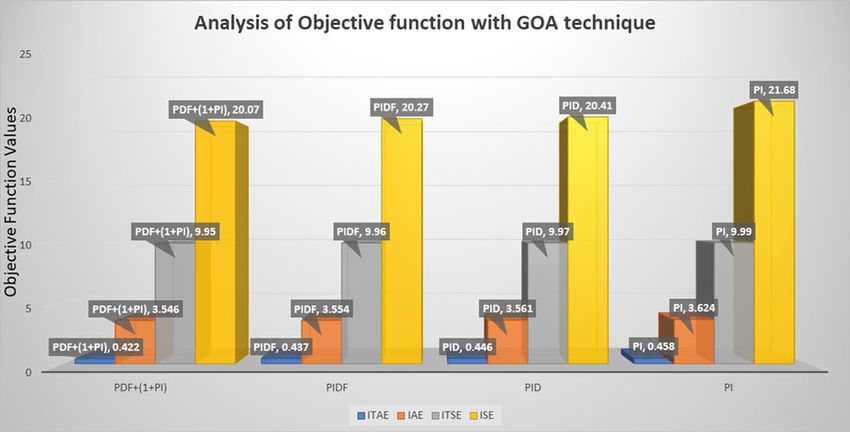
Nayak et al. Protection and Control of Modern Power Systems   (2021) 6:8                           Page 10 of 15

 Fig. 9 Dynamic responses of FACTS devices with GOA optimized PDF+(1 + PI) controller and 1% SLP
Nayak et al. Protection and Control of Modern Power Systems      (2021) 6:8                                                Page 11 of 15

Table 4 Peak deviation and settling time for effectiveness measurement of FACTS devices
Element        Peak Overshoot (+)                             Peak Undershoot (−)                          Settling Time in seconds
               SSSC       TCPS        TCSC        IPFC        SSSC        TCPS       TCSC       IPFC       SSSC    TCPS    TCSC       IPFC
Δf1 (Hz)       0.003381   0.001650    0.001122    0.000740    0.018378    0.009548   0.006447   0.007415   45.70   41.39   39.48      34.22
Δf2 (Hz)       0.003345   0.001582    0.001114    0.000735    0.018384    0.009535   0.006459   0.007567   45.83   43.09   38.78      37.07
Δf3 (Hz)       0.003297   0.001656    0.001104    0.000551    0.018382    0.009555   0.006431   0.006845   44.70   43.32   40.28      38.12
ΔPtie1–2(pu)   0.001965   0.001788    0.001699    0.001674    0.011174    0.010781   0.009131   0.008423   46.58   43.38   41.91      42.68
ΔPtie2–3(pu)   0.001898   0.001670    0.001623    0.001458    0.011426    0.010368   0.010293   0.010127   44.88   42.62   41.31      37.84
ΔPtie3–1(pu)   0.001758   0.001689    0.001661    0.001467    0.011223    0.010846   0.010547   0.010113   47.22   44.36   41.76      40.96

 Fig. 10 Dynamic responses of IPFC with different locations and SLP values
Nayak et al. Protection and Control of Modern Power Systems (2021) 6:8 Page 12 of 15
Table 5 Peak deviation and settling time for GOA optimized PDF plus (1 + PI) controller with IPFC and different SLP values
Condition Peak Overshoot (+) Peak Undershoot (−) Settling Time in seconds
Δf1 (Hz) Δf2 (Hz) ΔPtie1–2(pu) Δf1 (Hz) Δf2 (Hz) ΔPtie1–2(pu) Δf1 (Hz) Δf2 (Hz) ΔPtie1–2(pu)
Without IPFC 0.011598 0.007540 0.001431 0.032582 0.026905 0.016016 38.73 3914 49.41
IPFC in 1–2 0.001170 0.001118 0.000647 0.019762 0.019764 0.011305 35.96 38.43 39.83
IPFC in 1–2-3 0.000740 0.000735 0.000551 0.007415 0.007567 0.006845 34.22 37.07 38.12
SLP 3% 0.002273 0.002125 0.002308 0.019367 0.019417 0.019322 58.15 56.92 58.12
SLP 5% 0.002358 0.002244 0.002399 0.029284 0.029264 0.029257 76.19 77.43 78.45
system with PDF plus (1 + PI) controller optimized by controller and GOA technique. This allows examination
GOA technique. of the robustness of the network when there is an uncer-
The dynamic responses of frequency deviation and tain nonlinearity, something that frequently occurs in a
power exchange across the tie-line are given in power system network.
Fig. 9(a)-(f), while the performance indices are given The dynamic responses for GOA-optimized PDF
in Table 4. From this analysis, it is noted that IPFC plus (1 + PI) controller for an IPFC enabled AGC
gives improved dynamic response (peak overshoot system is shown in Fig. 10(a)-(c) with different loca-
and undershoot and settling time) over other pro- tions of IPFC and SLP values. The performance at-
posed FACTS devices. Compared to SSSC, TCPS tributes are given in Table 5. From these, it can be
and TCSC, the improved settling times of frequency concluded that the IPFC with each area stabilizes
deviation Δf1 with IPFC and the proposed GOA the frequency and limits the oscillation of the power
tuned PDF plus (1 + PI) controller are 25.12%, flow.
17.32% and 13.32%, respectively, while for Δf2, they
are 19.11%, 13.97% and 4.40%, respectively. For Δf3, 4.5 Sensitivity analysis
the corresponding settling time improvements are In this section, sensitivity analysis is carried out for
14.72%, 12% and 5.36%, respectively. For ΔPtie1–2, the proposed GOA optimized PDF plus (1 + PI) con-
the improved settling times of frequency deviation troller for the IPFC-enabled AGC system. The
with IPFC compared to SSSC, TCPS and TCSC are optimum controller gains are evaluated at nominal
10.02%, 3.38% and 1.8%, respectively, while the cor- loading conditions with 1% SLP to the wide variation
responding respective improvements are 15.68%, of system parameters. The GOA runs for each possi-
11.21% and 8.39% for ΔPtie2–3, and 13.25%, 7.66% bility of system parameter setting and with tuned pa-
and 1.91% for ΔPtie3–1. rameters system performance index are evaluated.
The dynamic response control indices are given in
Table 6. The controller parameters are quite close to
4.4 Effectiveness of IPFC at a different location with SLP each other which validates the robustness of the
In this section, the multi-thermal power system network complete framework as the proposed method. From
is tested with different locations of IPFC. It is also verified every aspect it exhibits an effective response in every
with hikes in SLP of 3% and 5% for the proposed possible condition.
Table 6 Peak deviation & Settling time for GOA optimized PDF plus (1 + PI) controller with different loading conditions
Loading Peak Overshoot (+) Peak Undershoot (−) Settling Time in seconds
Condition
Δf1 (Hz) Δf2 (Hz) ΔPtie1–2(pu) Δf1 (Hz) Δf2 (Hz) ΔPtie1–2(pu) Δf1 (Hz) Δf2 (Hz) ΔPtie1–2(pu)
Nominal 0.000740 0.000735 0.000551 0.007415 0.007567 0.006845 34.22 37.07 38.12
+ 25% 0.001748 0.001654 0.001726 0.009492 0.009536 0.009445 41.92 41.74 42.20
- 25% 0.001600 0.001611 0.001633 0.009544 0.009483 0.009418 41.53 40.91 41.53
+ 50% 0.002308 0.002278 0.002236 0.009575 0.009551 0.009554 42.02 41.89 42.23
- 50% 0.001582 0.001576 0.001586 0.009531 0.009548 0.009493 40.98 41.48 41.84
+ 75% 0.001844 0.001802 0.001852 0.009551 0.009475 0.009548 41.23 41.96 42.39
- 75% 0.001485 0.001553 0.001513 0.009547 0.009546 0.009557 40.58 40.35 41.02Nayak et al. Protection and Control of Modern Power Systems (2021) 6:8 Page 13 of 15
AB/SIMULINK and OPAL-RT based Real-Time
Simulator (RTS) are shown in Fig. 12(a) and (b). It
can be seen that the MATLAB/SIMULINK results
match well with those from OPAL-RT real-time
simulation.
5 Conclusion
A 3-area thermal unit fitted with a reheat turbine is consid-
ered in this paper. The Grasshopper optimization algorithm
is used in AGC to optimize the PI, PID, PIDF and the pro-
Fig. 11 OPAL-RT OP5700 RCP/HIL FPGA real-time simulator posed PDF plus (1 + PI) controllers. First, statistical analysis
is carried out to evaluate the effectiveness of GOA in test
functions. Several FACTS devices such as SSSC, TCPS,
TCSC and IPFC in association with PDF plus (1 + PI) opti-
4.6 Validation by OP5700 RCP/HIL FPGA real-time mized by GOA in AGC 3-area systems are tested. Improve-
simulator ments in the ITAE error with the proposed GOA tuned
The OPAL-RT OP5700 RCP/HIL FPGA real-time PDF plus (1 + PI) controller compared to the PIDF, PID and
simulator is shown in Fig. 11 which is used for real- PI are 3.43%, 5.38% and 7.86%, respectively. The effectiveness
time validation of the proposed research. This is per- of GOA is justified by comparing the dynamic responses
formed for practical feasibility testing. The OPAL- with GA and PSO, where respective improvements of
RT considers the delay and error nonlinearity distur- 12.26% and 17.57% in the ITAE error with the proposed
bances which inherently exist but are neglected in GOA tuned PDF plus (1 + PI) controller are achieved. It is
conventional off-line simulations [26]. The OPAL-RT also observed that the IPFC gives improved dynamic re-
allows researchers to authenticate their work in real- sponse (peak overshoot and undershoot, and settling time)
time irrespective of complexity. The important fea- in comparison with other considered FACTS devices.
tures of OPAL-RT are code parallelization, Simulink The robustness of the proposed strategy is estimated by
integration, customizable dashboard, communication various sensitivity analyses. Dynamic behaviors due to differ-
protocols and I/O flexibility. The steps of real-time ent SLP and loading conditions are compared and sensitiv-
validation include the initialization of the Simulink ity analysis reveals that a GOA-tuned PDF plus (1 +
model via OPAL-RT lab, the transformation of the PI) controller-fitted IPFC offers robustness in all
model into RT application, running the model using respects. Finally, the proposed GOA-tuned PDF plus
multiple cores and finally data acquisition using the (1 + PI) controller fitted IPFC approach is authenti-
graphical interface. The frequency deviation (Δf1) cated by OPAL-RT based simulations in a real-time
and tie-line power response (ΔPtie 1–2) from MATL environment.
Fig. 12 OPAL-RT OP5700 RCP/HIL FPGA real-time simulator vs MATLAB/SIMULINK resultsNayak et al. Protection and Control of Modern Power Systems (2021) 6:8 Page 14 of 15 1 Appendix Table 7 Nominal parameters of the system: system frequency f = 60 Hz, Tgi = 0.08 s, Tti = 0.3 s; Tri = 10 s; Kri = 0.5; Kpi = 120 Hz/pu MW; Tpi = 20 s; T12 = 0.086 pu MW/rad; Hi = s; Di = 8.33X10⁻³ pu MW/Hz; βi = 0.425 pu MW/Hz; Ri = 2.4 pu Hz/MW; loading = 50%; TSSSC = 0.03 s; KSSSC = 0.1802; Kφ = 1.5 rad/Hz; TPS = 0.1 s; TTCSC = 0.015 s; TIPFC = 0.01 s Terminology i Control area number i (1,2,3) m, n Grasshopper index Xm location of mth Grasshopper Sm correlation Gm gravitational strength on the mth Grasshopper Am wind abeyance C Coefficient of the comfort zone KSSSC SSSC gain TSSC SSSC time constant TTCPS TCPS time constant Kφ TCPS gain Δφ phase-shifting angle TTCSC TCSC time constant TIPFC IPFC time constant Hi inertia constant of control area i (s) ΔPLi load increments in (p.u) ΔPgi generation increments in (p.u) Di ΔPLi /Δfi (pu/Hz) T12, T23, T13 synchronizing factors Ri speed regulation factor of control area i (Hz/pu MW) Tgi the time constant of reheat governor control area i (s) Kri reheat coefficient of control area i Tri Reheat time constant of area i (s) Tti the turbine time constant of control area i (s) Bi frequency bias constant of area i Tpi 2Hi/ f * Di Kpi 1/Di (Hz/pu) KPi proportional gain of PI, PID, PIDF, and PIDF plus (1 + PI) controller in the control area i KIi integral gain of integral, PI, PID, PIDF and PIDF plus (1 + PI) controller in control area i KDi derivative gain of PID, PIDF, and PIDF plus (1 + PI) controller in the control area i KPPi the proportional gain of (1 + PI) controller in the control area i Ni filter coefficient of PIDF & PDF controller in control area i D(s) estimated derivative term = s/ 1 + Ns βi control area frequency response characteristics of area I (AFRC) = Di + 1/Ri Δfi frequency incremental of control area i (Hz) ΔPgi Generation increments of control area i (p.u) ΔPtie i-j tie-line power increment among control area i and area j (p.u) T simulation time (s)
Nayak et al. Protection and Control of Modern Power Systems                                (2021) 6:8                                                                   Page 15 of 15

                                                                                                   12. Pradhan, P. C., Sahu, R. K., & Panda, S. (2015). Firefly algorithm optimized
Acknowledgements                                                                                       fuzzy PID controller for AGC of multi-area multi-source power systems with
Not applicable.                                                                                        UPFC and SMES. Engineering Science and Technology an International
                                                                                                       Journal, 2015, 338–354. https://doi.org/10.1016/j.jestch.2015.08.007.
Authors’ contributions                                                                             13. Sahu, R. K., Panda, S., & Yegireddy, N. K. (2014). A novel hybrid DEPS
The first author developed the models and obtained the results. The second                             optimized fuzzy PI/PID controller for load frequency control of multi-area
author implemented the optimization algorithm and tested on OPAL-RT. The                               interconnected power systems. Journal of Process Control, 24(10), 1596–1608.
third author suggested the controller and validated the manuscript. The au-                            https://doi.org/10.1016/j.jprocont.2014.08.006.
thor(s) read and approved the final manuscript.                                                    14. Saikia, L. C., Nanda, J., & Mishra, S. (2011). Performance comparison of
                                                                                                       several classical controllers in AGC for multi-area interconnected thermal
                                                                                                       system. Electrical Power and Energy Systems, 33, 394–401. https://doi.org/10.1
Author’s information
                                                                                                       016/j.ijepes.2010.08.036.
Pratap Chabdra Nayak is a Ph.D research Scholar in the Department of
                                                                                                   15. Sahu, R. K., Panda, S., & Rout, U. K. (2013). DE optimized parallel 2-DOF PID
Electrical Engineering, VSSUT, Burla, 768018, Odisha, India. Ramesh Chandra
                                                                                                       controller for load frequency control of power system with governor dead-
Prusty is working as Assistant Professor in the Department of Electrical
                                                                                                       band nonlinearity. Electrical Power and Energy Systems, 49, 19–33. https://doi.
Engineering, VSSUT, Burla, 768018, Odisha, India. Sidhartha Panda is working
                                                                                                       org/10.1016/j.ijepes.2012.12.009.
as Professor in the Department of Electrical Engineering, VSSUT, Burla,
                                                                                                   16. Nayak, P. C., Prusty, U. C., Prusty, R. C., & Barisal, A. K. (2018). Application of
768018, Odisha, India.
                                                                                                       SOS in fuzzy based PID controller for AGC of multi-area power system. IEEE
                                                                                                       Conference on Technologies for Smart – City Energy Security and Power, 1, 1–
Funding
                                                                                                       6. https://doi.org/10.1109/ICSESP.2018.8376709.
Not applicable.
                                                                                                   17. Demiroren, A., & Yesil, E. (2004). Automatic generation control with fuzzy
                                                                                                       logic controllers in the power system including SMES units. Electrical Power
Availability of data and materials
                                                                                                       and Energy Systems, 26, 291–305. https://doi.org/10.1016/j.asej.2014.03.011.
Not applicable.
                                                                                                   18. Nayak, P. C., Sahoo, A., Balabantaray, R., & Prusty, R. C. (2018). Comparative
                                                                                                       study of SOS & PSO for fuzzy based PID controller in AGC in an integrated
Competing interests                                                                                    power system. IEEE Conference on Technologies for Smart – City Energy
The author declares that they have no competing interests.                                             Security and Power, 1, 1–6. https://doi.org/10.1109/ICSESP.2018.8376700.
                                                                                                   19. Dash, P., Saikia, L. C., & Sinha, N. (2015). Automatic generation control of
Received: 19 March 2020 Accepted: 8 February 2021                                                      multi area thermal system using bat algorithm optimized PD–PID Cascade
                                                                                                       controller. Electrical Power and Energy Systems, 68, 364–372. https://doi.org/1
                                                                                                       0.1016/j.ijepes.2014.12.063.
References                                                                                         20. Padhy, S., & Panda, S. M. (2017). A modified GWO technique-based cascade
1. Elgerd, O. L. (2000). Electric energy systems theory – An introduction, Tata Mc Graw                PI-PD controller for AGC of power systems in presence of plug-in electric
    Hill, New Delhi.J. Clerk Maxwell, a treatise on electricity and magnetism, (vol. 2, 3rd ed.,       vehicles. Engineering Science and Technology, 20(2), 427–442. https://doi.
    pp. 68–73). Oxford: Clarendon, 1892. https://doi.org/10.1007/978-1-4615-5997-9_6.                  org/10.1016/j.jestch.2017.03.004.
2. Fosha, C. and Elgerd, O.I. (1970), “The megawatt-frequency control problem: A                   21. Sahu, P. C., Prusty, R. C., & Panda, S. (2019). A gray wolf optimized FPD plus (1+
    new approach via optimal control theory”, IEEE transactions on power apparatus                     PI) multistage controller for AGC of multisource non-linear power system.
    and systems, PAS-89 4, 563-577, DOI: https://doi.org/10.1109/TPAS.1970.292603.                     World Journal of Engineering. https://doi.org/10.1108/WJE-05-2018-0154.
3. Kundur, P. (2006). Power System Stability and Control. New Delhi: Tata                          22. Nayak, P. C., Prusty, R. C., & Panda, S. (2020). Grasshopper optimization
    McGraw, https://www.mheducation.co.in/power-system-stability-and-                                  algorithm of multistage PDF+(1+ PI) controller for AGC with GDB & GRC
    control-9780070635159-india.                                                                       nonlinearity of dispersed type power system. International Journal of
4. Hingorani, N. G., & Gyugyi L. (2000). Understanding FACTS: Concepts and                             Ambient Energy, 1–21. https://doi.org/10.1080/01430750.2019.1709897.
    Technology of Flexible AC Transmission Systems. Wiley-IEEE Press, https://                     23. Dash, P., Saikia, L. C., & Sinha, N. (2015). Comparison of performances of
    ieeexplore.ieee.org/servlet/opac?bknumber=5264253.                                                 several FACTS devices using cuckoo search algorithm optimized 2DOF
5. Praghnesh, B., Ranjit, R., & Ghoshal, S. P. (2011). Comparative performance                         controllers in multi-area AGC. Electrical Power and Energy Systems, 65, 316–
    evaluation of SMES–SMES, TCPS–SMES, and SSSC–SMES controllers in                                   324. https://doi.org/10.1016/j.ijepes.2014.10.015.
    automatic generation control for a two-area hydro–hydro system.                                24. Tasnin, W. & Saikia, L. C. (2019). Impact of renewables and FACT device on
    International Journal of Electrical Power & Energy Systems, 33(10), 1585–1597.                     deregulated thermal system having sine cosine algorithm optimised
    https://doi.org/10.1016/j.ijepes.2010.12.015.                                                      fractional order cascade controller. IET Renewable Power Generation, 13(9),
6. Sahu, P. R., Hota, P. K., & Panda, S. (2018). Power system stability                                1420–1430. https://doi.org/10.1049/iet-rpg.2018.5638.
    enhancement by fractional-order multi-input SSSC based controller                              25. Saremi, S., Mirjalili, S., & Lewis, A. (2017). Grasshopper optimization
    employing whale optimizing algorithm. Electrical Systems and Information                           algorithm: Theory and application. Advances in Engineering Software, 105,
    Technology, 5(3), 326–336. https://doi.org/10.1016/j.jesit.2018.02.008.                            30–47. https://doi.org/10.1016/j.advengsoft.2017.01.004.
7. Praghnesh, B., Ranjit, R., & Ghoshal, S. P. (2012). Coordinated control of TCPS                 26. Khooban, M. H. (2017). Secondary load frequency control of time-delay
    and SMES for frequency regulation of interconnected restructured power                             stand-alone micro-grids with electric vehicles. IEEE Transactions on Industrial
    systems with dynamic participation from DFIG based wind farms. Renew                               Electronics, 65(9), 7416–7422. https://doi.org/10.1109/TIE.2017.2784385.
    Energy, 40, 40–50. https://doi.org/10.1016/j.renene.2011.08.035.
8. Chidambaram, I. A., & Paramasivam, B. (2012). Control performance
    standards-based load frequency controller considering redox flow batteries
    coordinate with an interline power flow controller. Journal of Power Sources,
    219, 292–304. https://doi.org/10.1016/j.jpowsour.2012.06.048.
9. Chidambaram, I. A., & Paramasivam, B. (2013). Optimized load-frequency
    simulation in restructured power system with redox flow batteries and
    interline power flow controller. International Journal of Electrical Power &
    Energy Systems, 50, 9–24. https://doi.org/10.1016/j.ijepes.2013.02.004.
10. Guo C., Tong L., & Wang Z. (2002). Stability control of TCSC between
    interconnected power networks. Proceedings. International Conference on
    Power System Technology, Kunming, China, 3, 1943–1946, https://doi.org/1
    0.1109/ICPST.2002.1067872.
11. Wadhai, S. D., & Ghawghawe, N. D. (2011). Power flow control by using TCSC
    controller in the power system. In i-COST electronics and communication
    conference proceeding, (pp. 27–33). https://doi.org/10.4010/2016.569.
You can also read