Hierarchical Face Parsing via Deep Learning
←
→
Page content transcription
If your browser does not render page correctly, please read the page content below
Hierarchical Face Parsing via Deep Learning

                   Ping Luo1,3                         Xiaogang Wang2,3                             Xiaoou Tang1,3
                          1
                              Department of Information Engineering, The Chinese University of Hong Kong
                           2
                               Department of Electronic Engineering, The Chinese University of Hong Kong
                              3
                                  Shenzhen Institutes of Advanced Technology, Chinese Academy of Sciences
               pluo.lhi@gmail.com                    xgwang@ee.cuhk.edu.hk                    xtang@ie.cuhk.edu.hk

                        Abstract

    This paper investigates how to parse (segment) facial
components from face images which may be partially oc-
cluded. We propose a novel face parser, which recasts
segmentation of face components as a cross-modality data
transformation problem, i.e., transforming an image patch
to a label map. Specifically, a face is represented hierarchi-
cally by parts, components, and pixel-wise labels. With this
representation, our approach first detects faces at both the
part- and component-levels, and then computes the pixel-
wise label maps (Fig.1). Our part-based and component-
                                                                        Figure 1. Hierarchical representation of face parsing (a). A face image
based detectors are generatively trained with the deep belief           is parsed by combining part-based face detection (b), component-based
network (DBN), and are discriminatively tuned by logistic               face detection (c), and component segmentation (d). There are four part-
regression. The segmentators transform the detected face                based detectors (left/right/upper/lower-half face) and six component-based
components to label maps, which are obtained by learning                detectors (left/right eye, left/right eyebrow, nose and mouth). Each compo-
                                                                        nent detector links to a novel component segmentator. (d) shows that the
a highly nonlinear mapping with the deep autoencoder. The               segmentators can transform the detected patches to label maps (1st , 2nd
proposed hierarchical face parsing is not only robust to par-           columns) and we obtain the fine-label maps after hysteresis thresholding
tial occlusions but also provide richer information for face            (3rd ). (e) is the image segmentation result (i.e., groups into 2 and 10 clus-
analysis and face synthesis compared with face keypoint de-             ters) obtained by normalized cut.
tection and face alignment. The effectiveness of our algo-
rithm is shown through several tasks on 2, 239 images se-               ing [2, 3, 17, 16, 5, 30, 14] or graphical models (e.g., M-
lected from three datasets (e.g., LFW [12], BioID [13] and              RF) [23, 15]. In this work, we study the problem from a
CUFSF [29]).                                                            new point of view and focus on computing the pixel-wise
                                                                        label map of a face image as shown in Fig.1 (d). It provides
1. Introduction                                                         richer information for further face analysis and synthesis
                                                                        such as 3D modeling [1] and face sketching [20, 19, 26],
   Explicitly parsing face images into different facial com-            comparing to the results obtained by face keypoint detec-
ponents implies analyzing the semantic constituents (e.g.,              tion and face alignment. This task is challenging and ex-
mouth, nose, and eyes) of human faces, and is useful for a              isting image segmentation approaches cannot achieve satis-
variety of tasks, including recognition, animation, and syn-            factory results without human interaction. An example is
thesis. All these applications bring new requirements on                shown in Fig.1(e). Inspired by the success of deep autoen-
face analysis—robustness to pose, background, and occlu-                coder [11], which can transform high-dimensional data into
sions. Existing works, including both face keypoint detec-              low-dimensional code and then recover the data from the
tion and face alignment, focus on localizing a number of                code within single modality, we recast face component seg-
landmarks, which implicitly cover the regions of interest.              mentation as a cross-modality data transformation problem,
The main idea of these methods is to first initialize the lo-            and propose an alternative deep learning strategy to direct-
cations of the landmarks (i.e., mean shape) by classification            ly learn a highly non-linear mapping from images to label
or regression, and then to refine them by template match-                maps.

                                                                    1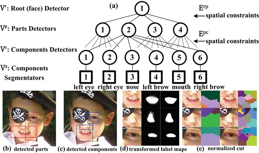
Figure 2. (a) and (b) define parts and components, which correspond to
the nodes in Fig.1 (a). Red points are the positions of parts (a) or compo-
nents (b). Red boxes are extracted image patches for training. (c) shows
the spatial relationship (i.e., orientation and position) between parts and
components.

    In this paper, we propose a hierarchical face parser. A                       Figure 3. Compare the alignment results of [16] ((a)-(d)) and ours ((e)-
face is represented hierarchically by parts, components, and                      (h)) when face images are partially occluded. Landmarks can be easily
                                                                                  obtained from the label maps obtained by our approach. The white boxes
pixel-wise labels (Fig.1 (a)). With this representation, our                      indicate the initial face detection results employed in [16]. It is not accurate
approach first detects faces at both the part- and component-                      in (a) due to occlusion. The blues boxes indicate the results of component
levels, and then computes the pixel-wise label maps. The                          detection. The red boxes indicate the results of part-based detectors em-
deformable part- and component-based detectors are incor-                         ployed in our approach.
porated by extending the conventional Pictorial model [9] in
                                                                                  popular to adopt discriminative approaches in facial analy-
a hierarchical fashion. As shown in Fig.1 (a), each node at
                                                                                  sis [23, 16, 5, 28]. For example, the BoRMaN method [23]
the upper three layers is a detector generatively pre-trained
                                                                                  and the Regression ASM [5] were proposed to detect facial
by Deep Belief Network (DBN) [10] and discriminative-
                                                                                  features or components using boosting classifiers on small
ly tuned with logistic regression (sec.3.2). At the bottom
                                                                                  image patches. A component-based discriminative search
layer, each node is associated with a component segmenta-
                                                                                  algorithm [16] extended the Active Appearance Model
tor, which is fully trained on a dataset with patch-label map
                                                                                  (AAM) [2] by combining the facial-component detectors
pairs by a modified deep autoencoder [11] (sec.3.3). Then,
                                                                                  and the direction classifiers, which predict the shifting di-
we demonstrate that with this model, a greedy search algo-
                                                                                  rections of the detected components.
rithm with a data-driven strategy is sufficient to efficiently
yield good parsing results (sec.3.1). The effectiveness of                           However, the aforementioned approaches have two
hierarchical face parsing is demonstrated through the appli-                      drawbacks. First, it is difficult for a single detector [25] to
cations of face alignment and detection of facial keypoints,                      accurately locate an occluded face for initialization. Thus,
and it outperforms the state-of-the-art approaches.                               the matching process fails to converge since the initial shape
                                                                                  is far away from the optimal solution as shown in Fig.3
1.1. Related Work                                                                 (a). Our method adopts multiple hierarchical deformable
    Recent approaches of scene parsing [22] provide an al-                        part- and component-based detectors and is more robust to
ternative view for face analysis, which is to compute the                         partial occlusions. Second, since face detection and shape
pixel-wise label maps [27]. This representation offers rich-                      matching are optimized alternately, we empirically observe
er information and robustness compared with the existing                          that even though the face components can be well detected,
face alignment and key point detection methods.                                   shape matching may still converge to a local minima be-
                                                                                  cause the correlation between shape and image appearance
    Active Shape Model (ASM) [3] is a well established and
                                                                                  is not well captured as shown in Fig.3 (a)(c). Our method
representative face alignment algorithm, and has many vari-
                                                                                  employs DBN to establish strong correlations between im-
ants [2, 17, 30]. They heavily rely on good initialization
                                                                                  ages and shapes by estimating the label maps directly from
and do not work well on images taken in unconstrained en-
                                                                                  the detected image patches. See Fig.1 (d) and Fig.3 (f)(h)
vironments, where shape and appearance may vary great-
                                                                                  for details.
ly. Starting with multiple initial shapes is a natural way to
overcome this problem [21, 15]. For instance, in order to be
robust to noise, the Markov Shape Model [15, 14] samples                          2. A Bayesian Formulation
many shapes by combining the local line segments and ap-
pearances as constraints. Although such methods reduce the                            Our hierarchical face parsing can be formulated under
dependence on initialization, they are computationally ex-                        a Bayesian framework, under which the detectors and seg-
pensive since a large number of examples have to be drawn;                        mentators can be explained as likelihoods, and spatial con-
otherwise, the matching may get stuck at local minimum.                           sistency can be explained as priors.
    To improve computational efficiency and to be robust                               Let I be an input image and L be a set of class labels of
to pose variations and background clutters, it has become                         all the detectors. Here, L = {r , pi , cj }i=1..4
                                                                                                                                j=1..6
                                                                                                                                       (see the upper

                                                                              2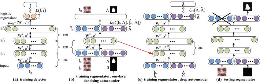
three layers of Fig.1 (a))1 . Under the Bayesian Framework,                       1) = N (o(br , bp ); μbr bp , Σbr bp )3 . Similarly, the prior of
our objective is to compute a solution θ that maximizes a                         p(E pc |V p ) can be factorized in the same way.
posterior probability, p(θ|I, L). Therefore,
                                                                                  2.2. The Scores of Detectors and Segmentators
          θ∗    =     arg max p(I, L|θ)p(θ)                            (1)           log p(I, L|θ) in Eq.1 can be explained as the sum of the
                =     arg max log p(I, L|θ) + log p(θ).                           scores of detectors and segmentators, and they are modeled
                                                                                  through DBNs and deep autoencoders respectively.
After taking “log”, the objective value is equivalent to a                           Let Ib be the image patch occupied by the bounding box
summation of a set of scores. In other words, our problem                         b. The likelihood probability, p(I, L|θ), can be factorized
is, given a facial image I, to hierarchically find the most                        into the likelihood of each node as,
possible parsing representation θ = (V r , V p , V c , V s , E),
which contains a set of nodes and edges. More specif-                                   p(I, L|θ) =                         p(I i , i |v i ) (3)
                                                                                                                             b
                         r/p/c           r/p/c r/p/c       r/p/c K                                          i∈{r,p1 ,...,p4 ,c1 ,...,c6 }
ically, V r/p/c = {vi             = (bi         , ρi    , λi    )}i=1                                                                       detector
are the root detector (K = 1), part detectors (K = 4),                                                      6

and component detectors (K = 6) respectively. E =                                                      ×             p(Ibsj |vjs ) .
(E rp , E pc ) indicates the spatial relations among the upper                                              j=1
                                                                                                                   segmentator
three layers. Here, we denote the component segmentators
as V s = {vis = (bsi , λsi , φi , Λi )}6i=1 . In particular, a node is            By applying the Bayes rule, we formulate the likeli-
described by a bounding box b, a binary variable λ ∈ {0, 1}                       hood of each detector as p(Ib , |v) = p(Ib ; ρdbn ) ×
that indicates whether this node is occluded (“off ”) or not                       p(|Ib , ρdbn ; ρreg )4 , and the likelihood of each component
(“on”), and a set of deep learning parameters ρ and φ2 . Λ                        segmentator as p(Ibs |v s ) = p(Ibs |Λs ; φsae )5 .
denotes the label map of the corresponding component.                                We model the first term of the detector’s likelihood by
                                                                                  DBN and discuss details in sec.3.2, and the second term
2.1. The Scores of Spatial Consistency                                            evaluates how likely a node should be located on a certain
                                                                                  image patch, is derived as below,
    Here, log p(θ) in Eq.1 is the score of spatial consistency,
which is modeled as a hierarchical pictorial structure.                           p(|Ib , b, λ, ρdbn ; ρreg ) ∝ exp{−  −f (Ib , ρdbn ; ρreg ) 1 },
    p(θ) is the prior probability, measuring the spatial com-                                                                                    (4)
patibility between a face and its parts, and also between                         where, given an image patch, f (·, ·) is a softmax function
each part and the components. Hence, we have p(θ) =                               that predicts its class label based on the learned parameters
p(E rp |v r )p(E pc |V p ), in which E rp = {< v r , vip > |∀vip ∈                ρdbn and ρreg . Furthermore, the likelihood of the segmen-
V p }4i=1 and E pc = {< vip , vjc > |∀vip ∈ V p , ∀vjc ∈                          tator has the following form6 and its parameters are learned
V c }j=1..6
     i=1..4 indicate two edge set (Fig.1 (a)). In this paper,
                                                                                  by deep autoencoders (sec.3.3),
we consider orientations and locations as two kinds of s-
                                                                                                                        p(Ibs |Λs , bs , λs ; φsae ) ∝      (5)
patial constraints. Therefore, the prior p(E rp |v r ) can be
factorized as,                                                                     exp{− min{g1 (Ibs |Λ       s
                                                                                                                  ; φsae ), ..., gk (Ibs |Λsk ; φsae )}}.
                                                                                 Here, we learn k deep autoencoders to estimate the label
 p(E rp |v r ) =                p(o(br , bpi )|λr )p(d (br , bpi )|λr ).
                                                                                  maps of a facial component and return the one with the min-
                  ∈E rp
                                                                                  imal cross-entropy error gk (·, ·)7 .
                                                         (2)
Here, the functions o(·, ·) and d (·, ·) respectively calcu-                      3. Hierarchical Face Parsing
late the relative angle and the normalized Euclidean dis-
tance between the centers of two bounding boxes br and                               Before we discuss the details, we first give an overview
bp . For example, in Fig.2 (c), we illustrate the spatial                         of our algorithm in sec.3.1. After that, we describe our
constraints of the right eye related to the left-half face.                       methods for learning the detectors in sec.3.2 and the seg-
We model the probabilities of these two spatial relations                         mentators in sec.3.3.
as Gaussian distributions. For instance, p(o(br , bp )|λr =                           3 When a node is “off ”, log p(o(br , bp )|λr = 0) = , where  is a

                                                                                  sufficiently small negative number.
    1 In our experiment (sec.3.4), r ∈ R2 , ∀p ∈ R5 , ∀c ∈ R7 , each               4 We drop the superscripts r/p/c here.
                                                 i            j
                                                                                      5 Note that the random variables b and λ are omitted for simplicity in
vector indicates class label of the node and has a 1-of-K representation.
                      c
Consider “mouth (5 )” as an example, the 5-th element is set to be 1 and         the derivation of the likelihoods.
all the other are 0, and the 7-th element denotes the class of background.            6 Eq.4 and Eq.5 are defined when λ = 1. Please refer to footnote 3 for
    2 ρ = (ρ
              dbn , ρreg ) includes the parameters for DBN and logistic re-       the situation that λ = 0.
gression. φ will be written as φae in later derivation which denotes the              7 g (·, ·) evaluates the cross-entropy error between the input image
                                                                                         k
parameters for the deep autoencoder.                                              patch and the reconstructed one under the k-th deep autoencoder.

                                                                              3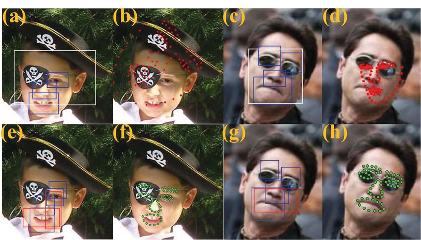
Algorithm 1: Hierarchical Face Parsing
                                                                                      Input: an image I and the class label set L
                                                                                      Output: label maps of facial components
                                                                                      1) Part-based detection:
                                                                                          (1) evaluate face or part detectors on I according to sec.3.2 in a
                                                                                      data-driven fashion
                                                                                          (2) hypothesize the face’s or parts’s position by calculating the
                                                                                      scores of spatial constraints (Eq.2) and detection (Eq.4)
                                                                                      2) Component segmentation:
                                                                                          (1) detect the components around the location proposed by 1)
                                                                                          (2) if a component is detected, then estimate its label map
                                                                                          (3) compute the scores according to sec.2.1 and Eq.5
                                                                                      3) Combine the scores of 1) and 2) together, if the final score is
                                                                                      larger than a threshold, then output the result.

                                                                                     Data-driven strategy 2. It is not necessary for us to enu-
Figure 4. The parsing process. In practice, we adopt the HOG features
from [6] and each testing image (a) is described by a HOG feature pyramid          merate all the combinations of the binary variable λ. If a
similar to [8]. (b) shows the scores of the “face” and the “right-half face”       node is not detectable, its λ is set to zero8 .
detectors. Note that the former one evaluates all positions while the latter
one evaluates only a small portion. (c) illustrates the scores of component        3.2. Learning Detectors
segmentators and the transformed label maps.
                                                                                      In this paper, we model our detectors by deep belief
3.1. Data-driven Greedy Search Algorithm                                           network (DBN), which is unsupervisedly pre-trained using
                                                                                   layer-wise Restricted Boltzmann Machine (RBM) [10] and
   Our data-driven greedy search algorithm can be separat-                         supervisedly fine-tuned for classification using logistic re-
ed into two steps: part-based face detection and component                         gression. Here, given image patches Ib as the training sam-
segmentation. For the first step, we assume that the nodes of                       ples (i.e., inputs in Fig.5 (a)), a DBN with K layers mod-
root and parts are visible (i.e., λ = 1), then we sequential-                      els the joint distribution between Ib and K hidden layers
ly evaluate their detectors with the sliding window scheme.                        h1 , ..., hk as follows:
Once a node has been activated, the other nodes, guided by
the data-driven information, will only search within a cer-                                                      p(Ib , h1 , ..., hk ; ρdbn ) =            (6)
tain range. For instance, as shown in Fig.4 (b), the root de-
                                                                                            K−2
tector tests all positions while the detector of the right-half                         (         p(hk |hk+1 ; ρdbn ))p(hK−1 , hK ; ρdbn ),
face tests only a small portion. After running all five de-                                  k=0
tectors, we combine the scores together, resulting in a good
hypothesis of the face’s position. Such strategy for object                        where Ib = h0 , p(hk |hk+1 ; ρdbn )) is a visible-given-
detection is fully evaluated in [8], where convincing results                      hidden conditional distribution of the RBM at level k, and
are reported. For the second step, we use the component                            p(hK−1 , hK ; ρdbn ) is the joint distribution at the top-level
detectors to search the components on the previously pro-                          RBM. Specifically, as illustrated in Fig.5 (a), learning the
posed location (Fig.4 (c)). If a component is activated, its                       paraments ρ = (ρdbn , ρreg ) of each detector includes two
corresponding segmentator is performed to output the label                         stages: first, ρdbn = {Wi , ui , zi }i=1..3 are estimated by
map. Eventually, the final score of the parsing is achieved                         pre-training the DBN using three RBMs layer-wisely. Then,
by summing up the scores of spatial constraints (sec.2.1),                         we randomly initialize ρreg = (Wr , ur ), and the initial-
detection (Eq.4), and segmentation (Eq.5). Moreover, the                           ized parameters ρreg along with the pre-trained parameters
result will be pruned by a threshold learned on a validation                       ρdbn are fine-tuned by logistic regression. This logistic re-
set. We summarize the algorithm in Algorithm.1.                                    gression layer maps the outputs of the last hidden layer to
   Data-driven strategy 1. To improve the search algorith-                         class labels and is optimized by minimizing the loss func-
                                                                                   tion between label hypothesis ()  and ground truth (). In
m, we solve a localization problem that is to determine the
angle and distance between a detected and an undetected                            the following, we discuss how to estimate ρdbn by RBM in
node. For example, as illustrated in Fig.2 (c), given the lo-                      details.
cation of the detected left-half face, we decide to predict the                        As the building block of DBN (see Fig.5 (a)), a RBM is
coordinates of the undetected right eye. We deal with this                         an undirected two-layer graphical model with hidden units
problem by training two regressors: the first one estimates                         (h) and input units (Ib ). There are symmetric connections
the angle α, and the second one finds the distance β. The                           (i.e., weights W) between the hidden and visible units, but
Support Vector Regression [4] is adopted to learn these two                           8 No need to evaluate the scores related to them. This is different

regressors.                                                                        from [8], where all part filters are visible.

                                                                               4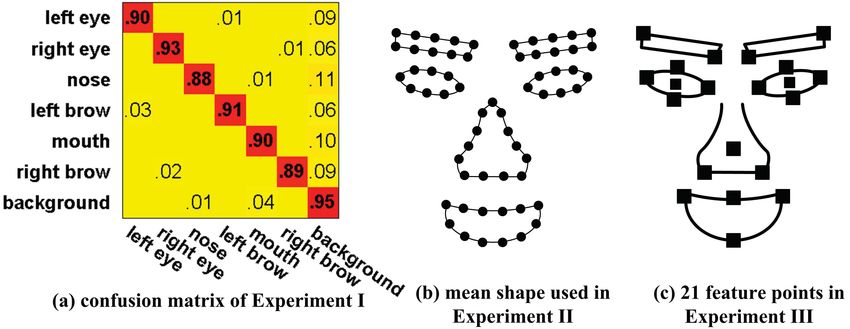
Figure 5. Illustration of learning process. We employ a four-layer DBN to model our detectors (a). The DBN is trained by layer-wise RBMs and tuned by
logistic regression. Then, we propose a deep training strategy containing two steps to train the segmentators: first, we train a deep autoencoder (c), whose
first layer are replaced by a one-layer denoising autoencoder (b). The deep autoencoder is tuned in one modality, while the one-layer autoencoder is tuned
in both modalities. Each trained segmentator can directly output the label map using an image patch as input (d).

no connections within them. It defines a marginal probabil-                           To learn a mapping from images to label maps, we must
ity over Ib using an energy model as below,                                      explore the correlations between them. Therefore, unlike
                                                                                 sec.3.2 where only image data are used for training, here
                     exp{zT Ib + uT h + hT WIb }                                we concatenate the images and ground truth label maps to-
  p(Ib ; ρdbn ) =                                               ,     (7)
                                           Z                                     gether as a training set. Since our purpose is to output label
                      h
                                                                                 map given only image as input, we augment this training set
where Z is the partition function and z, u are the offset vec-                   by adding samples that have zero values of the label map
tor for input units and hidden units respectively. In our case,                  and original values of the image (see Fig.5 (b)(c)). In other
the conditional probabilities of p(h|I) and p(I|h) can be                        words, half of the training data has only image (i.e., (Ib , 0)),
simply modeled by products of Bernoulli distributions:                           while the other half has both image and ground truth la-
                                                                                 bel map (i.e., (Ib , Λ)). Similar strategy is adopted by [18],
            p(hi = 1|I) = sigm(ui + Wi· I),                           (8)        which learns features by using data from different modal-
            p(Ij = 1|h) = sigm(zj + W·j
                                     T
                                        h).                                      ities in order to improve the performance of classification
                                                                                 performed in single modality.
sigm(·) is the sigmoid function. The parameters ρdbn can
                                                                                     1) Deep Autoencoder. As shown in Fig.5 (c), we estab-
be estimated by taking gradient steps determined by the
                                                                                 lish a four-layer deep autoencoder, whose parameters ρae
contrastive divergence [10].
                                                                                 can be defined as {Wi , ui , zi }i=1..2 . The weights and off-
3.3. Learning Segmentators                                                       set vector for the first layer are achieved by a one-layer de-
                                                                                 noising autoencoder introduced in step 2). We estimate the
    In this section, we introduce a deep learning approach                       weights of the second layer by RBM, and the weights of the
for training the component segmentators, which transfor-                                                                                     T
                                                                                 upper two layers are tied similar to [11] (i.e., W3 = W2 ,
m image patches to label maps. The data transforma-                                           T
                                                                                 W4 = W1 ). Then, the whole network is tuned in single
tion problem has been well examined by deep architectures
                                                                                 modality, that is minimizing the cross-entropy error LH be-
(i.e., multilayer network) in previous methods. Neverthe-
                                                                                 tween the outputs at the top layer (i.e., reconstructed label
less, they mainly focus on single modality, such as deep                                 and the targets (i.e., ground truth label maps Λ).
                                                                                 maps Λ)
autoencoder [11] and deep denoising autoencoder [24].
The former one encodes high-dimensional data into low-                              2) One-layer denoising autoencoder. Modeling the low-
dimensional code and decodes the original data from it,                          level relations between data from different modalities is cru-
while the latter one learns a more robust encoder and de-                        cial but not a trivial task. Therefore, to improve the per-
coder which can recover the data even though they are heav-                      formance of the deep network, we specially learn its first
ily corrupted by noise. By combining and extending the ex-                       layer with a denoising autoencoder [24] as shown in Fig.5
isting works, we propose a deep training strategy containing                     (b). Such shallow network is again pre-trained by RBM, but
two portions: we train 1) a deep autoencoder, whose first                         tuned in both modalities (i.e., images and label maps). Note
layer is replaced by 2) a one-layer denoising autoencoder.                       that in the fine-tuning stage, only the images and the ground
In the following, we explain how to generate the training                        truth label maps are used as the targets as shown at the top
data first, and then discuss the above two steps in detail.                       layer of Fig.5 (b).

                                                                            5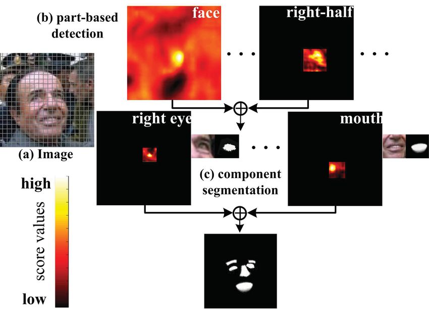
Overall, with these two steps, each component segmen-                          collect a dataset from internet and compare the face align-
tator learns a highly non-linear mapping from images to la-                       ment results with a state-of-the-art method, the Component-
bel maps. The testing procedure is illustrated in Fig.5 (d),                      based Discriminative Search (CBDS) [16]; Third, we com-
where we delete the unused image data in the output. Thus,                        pare with two leading approaches (i.e., BoRMaN [23] and
the deep network indeed outputs a label map given an image                        Extended ASM (eASM) [17]) of feature point extractions.
patch.                                                                            This experiment is conducted on the BioID [13] database;
                                                                                  Finally, to further evaluate the generalization power, we
3.4. Implementation Details
                                                                                  carry out a segmentation task on the CUHK Face Sketch
    In this section, we sketch several details for the sake of                    FERET Database (CUFSF) [29]. Note that for all these ex-
reproduction.                                                                     periments, our model is trained on the LFW as outlined in
    Training Detectors. We randomly select 3, 500 images                          sec.3.4.
from the Labeled Faces in the Wild (LFW) [12] database.                              Experiment I: performance of segmentators. We
We then randomly perturb each extracted image patch (see                          test our segmentators with a 7-classes facial image pars-
red boxes in Fig.2 (a)(b)) by translation, rotation, and scal-                    ing experiment, which is to assign each pixel a class label
ing. Therefore, for each category, we totaly have 42, 000                         (e.g., left/right eye, left/right brow, nose, mouth, and back-
training patches. Multi-label classification strategy is em-                       ground). First, we randomly select 300 images from the
ployed so that training three DBNs are enough (i.e., one                          LFW database, and all the label maps of these images are
for face detector, one for part detectors, and the other for                      well-labeled by hand. Then, our data-driven greedy search
component detectors). More specifically, as shown in Fig.5                         algorithm is performed on these images to achieve the re-
(a), we construct a 3-layers deep architecture and the unit                       constructed label maps, from which we obtain the final re-
numbers are 2 times, 3 times, and 4 times of the input size                       sults after hysteresis thresholding. Fig.7 (a) shows the con-
respectively. We supervisedly tune three DBNs with 2 out-                         fusion matrix, in which accuracy values are computed as the
puts, 5 outputs, and 7 outputs at the top layer respectively.                     percentage of image pixels assigned with the correct class
To construct the examples of the background category, we                          label. The overall pixel-wise labeling accuracy is 90.86%.
crop 105, 000 patches from the background for each DBN.                           It demonstrates the ability of the learned segmentators on
All examples of the three DBNs are normalized to 64 × 64,                         the segmentation of facial components. Several parsing re-
64 × 32, and 32 × 32 respectively. We use 9 gradient orien-                       sults are visualized in Fig.10 (a).
tations and 6 × 6 cell size to extract the HOG feature.

Figure 6. (a) Different translations and orientations are imposed in our
training data. (b) shows how to deal with pose variations. We first separate
the training data by K-means, then learn one deep autoencoder on each             Figure 7. (a) shows the confusion matrix of Experiment I. (b) and (c) are
cluster.                                                                          the face models for Experiment II and Experiment III respectively.
   Training Segmentators. We choose anther 500 images                                 Experiment II: face alignment. The purpose of our
from the LFW [12] database, whose label maps are manual-                          second experiment is to test our algorithm on the task of
ly annotated. Nevertheless, in order to cover variant poses,                      face alignment compared with the CBDS method, which
we import fluctuations on position and orientation for each                        was trained on many public databases including LFW over
example as illustrated in Fig.6 (a). Similarly, all training                      4, 000 images. In the spirit of performing a database in-
patches are fixed at 32 × 32 and described by HOG fea-                             dependent test, we collect a testing dataset containing 118
ture. In order to account for pose variations, we train a set                     facial images from Google Image Search and Flickr. This
of 4-layers deep autoencoders for each component, which is                        dataset is challenging due to occlusion, background clutters,
obtained by first applying K-means on the label maps and                           pose and appearance variations. Some examples are given
then training one autoencoder on each cluster. Empirically,                       in Fig.8.
we set K = 15 (Fig.6 (b)).
                                                                                      To apply our method to face alignment, we first obtain
                                                                                  the label map with the data-driven greedy search algorithm.
4. Experiments
                                                                                  Then a mean shape as illustrated in Fig.7 (b) is fitted to the
   We conduct four experiments to test our algorithm. First,                      label map by minimizing the Procrustes distance [7]. Note,
we perform face parsing on the LFW [12] database to e-                            the mean shape we used is different from the CBDS’s. To
valuate the performance of our segmentators; Second, we                           allow a fair comparison, we thus exclude the bridge of the

                                                                              6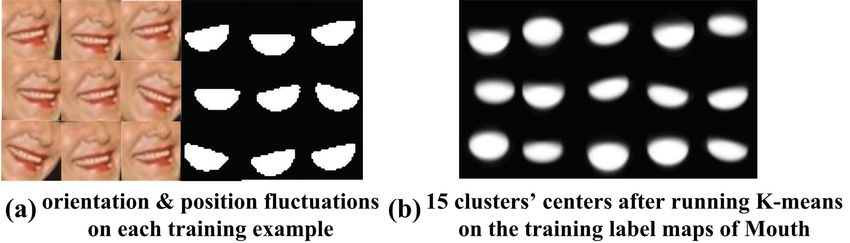
1                                                           1

                                                                                                       0.9                                                       0.9

                                                                                                       0.8                                                       0.8

                                                                                                       0.7                                                       0.7

                                                                                                                                                      Images Portion
                                                                                          Images Portion
                                                                                                       0.6                                                       0.6

                                                                                                       0.5                                                       0.5

                                                                                                       0.4                                                       0.4

                                                                                                       0.3                                                       0.3

                                                                                                                                      BoRMaN
                                                                                                       0.2                                                       0.2                              Ours
                                                                                                                                      eASM
                                                                                                                                      Ours                                                        BoRMaN
                                                                                                       0.1                                                       0.1

                                                                                                           0                                                           0
                                                                                                            0   0.02 0.04 0.06 0.08 0.1   0.12 0.14                     0   0.02   0.04   0.06 0.08 0.1   0.12   0.14
                                                                                                                            Distance                                                        Distance

    Figure 8. Some samples in the testing dataset of Experiment II.            Figure 9. Comparisons of the cumulative error distribution of point-wise
                                                                               error measured on set A (left) and set B (right) respectively.
nose in our shape, and the inner lips and profiles of CBDS
are also excluded. To yield a better alignment, we permit                      all the points except for the facial profile and eyelids. Fig.9
sightly non-rigid deformation of each landmark during the                      (left) shows that our approach outperforms these two meth-
matching procedure. We summarize the results in Table 1,                       ods.
which shows the percentage of images with the root mean                            Part 2. We then compare our method with BoRMaN on
squared error (RMSE) less than the specific thresholds. As                      set B, where the images are partially occluded. The results
we can see, our algorithm achieves better results than CBD-                    are shown in Fig.9 (right). When occlusions are present-
S. This is because our part-based detectors are very robust                    ed, we demonstrate that our approach provides significantly
to occlusions and pose variations, and the segmentators can                    better results. Some results are plotted in Fig.10 (c).
directly estimate the label map without a separated template                       Experiment IV: facial component segmentation. To
matching process. The results of our method on several par-                    further show that our algorithm can generalize to different
tially occluded faces are shown in Fig.10 (b).                                 facial modality, we conduct a 7-classes segmentation test on
                                                                               100 face sketch images selected from the CUFSF database.
  Methods \ RMSE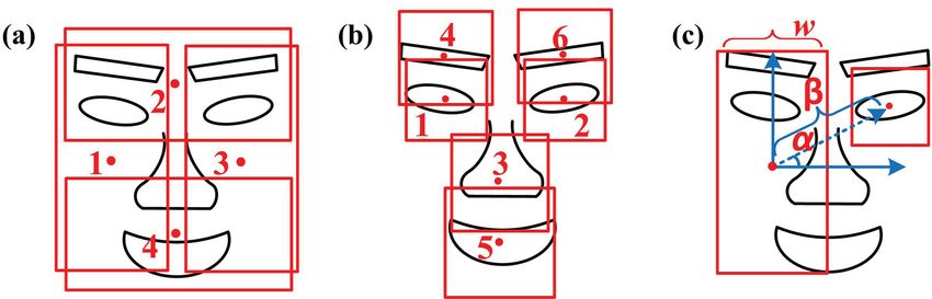
Figure 10. Demonstration of our results. The parsing results of Experiment I are shown in (a), where the 1st column is the original images, and the
2nd , 3rd columns are the transformed label maps and the ground truth respectively. (b) is the aligned faces of Experiment II. (c) visualizes some results of
facial feature extraction on the partially occluded set B. (d) is the segmentation results on face sketches.

 [2] T. Cootes, G. Edwards, and C. Taylor. Active appearance models.              [16] L. Liang, R. Xiao, F. Wen, and J. Sun. Face alignment via
     ECCV, 1998.                                                                       component-based discriminative search. ECCV, 2008.
 [3] T. Cootes, C. Taylor, and J. Graham. Active shape models their train-        [17] S. Milborrow and F. Nicolls. Locating facial features with an extend-
     ing and application. Computer Vision and Image Understanding,                     ed active shape model. ECCV, 2008.
     1995.                                                                        [18] J. Ngiam, A. Khosla, M. Kim, J. Nam, H. Lee, and A. Y. Ng. Multi-
 [4] N. Cristianini and J. Shawe-Taylor. An introduction to support vec-               modal deep learning. ICML, 2011.
     tor machines: and other kernel-based learning methods. Cambridge             [19] X. Tang and X. Wang. Face sketch synthesis and recognition. ICCV,
     University Press, 2000.                                                           2003.
 [5] D. Cristinacce and T. Cootes. Boosted regression active shape mod-           [20] X. Tang and X. Wang. Face sketch recognition. IEEE Transactions
     els. BMVC, 2007.                                                                  on Circuits and Systems for Video Technology, 2004.
 [6] N. Dalal and B. Triggs. Histograms of oriented gradients for human           [21] J. Tu, Z. Zhang, Z. Zeng, and T. Huang. Face localization via hier-
     detection. CVPR, 2005.                                                            archical condensation with fisher boosting feature selection. CVPR,
 [7] I. Dryden and K. Mardia. Statistical shape analysis. John Wiley and               2004.
     Son, Chichester, 1998.                                                       [22] Z. Tu, X. Chen, A. Yuille, and S. Zhu. Image parsing: unifying
 [8] P. Felzenszwalb, R. Girshick, and D. McAllester. Cascade object                   segmentation, detection and recognition. IJCV, 2005.
     detection with deformable part models. CVPR, 2010.                           [23] M. Valstar, B. Martinez, X. Binefa, and M. Pantic. Facial point de-
 [9] P. Felzenszwalb and D. Huttenlocher. Pictorial structures for object              tection using boosted regression and graph models. CVPR, 2010.
     recognition. International Journal of Computer Vision, 2005.                 [24] P. Vincent, H. Larochelle, I. Lajoie, Y. Bengio, and P. Manzagol.
                                                                                       Stacked denoising autoencoders: Learning useful representations in
[10] G. Hinton, S. Osindero, and Y. Teh. A fast learning algorithm for
                                                                                       a deep network with a local denoising criterion. Journal of Machine
     deep belief nets. Neural Computation, 2006.
                                                                                       Learning Research, 2010.
[11] G. Hinton and R. Salakhutdinov. Reducing the dimensionality of
                                                                                  [25] P. Viola and M. Jones. Robust real-time face detection. IJCV, 2004.
     data with neural networks. Science, 2006.
                                                                                  [26] X. Wang and X. Tang. Face photo-sketch synthesis and recognition.
[12] G. Huang, M. Ramesh, T. Berg, and E. Miller. Labeled faces in
                                                                                       TPAMI, 2009.
     the wild: A database for studying face recognition in unconstrained
                                                                                  [27] J. Warrell and S. Prince. Labelfaces: Parsing facial features by mul-
     environments. Technical Report, 2007.
                                                                                       ticlass labeling with an epitome prior. ICIP, 2009.
[13] O. Jesorsky, K. Kirchberg, and R. Frischholz. Robust face detection
                                                                                  [28] H. Wu, X. Liu, and G. Doretto. Face alignment via boosted ranking
     using the hausdorff distance. Lecture Notes in Computer Science,
                                                                                       model. CVPR, 2008.
     2001.
                                                                                  [29] W. Zhang, X. Wang, and X. Tang. Coupled information-theoretic
[14] L. Liang, F. Wen, X. Tang, and Y. Xu. An integrated model for
                                                                                       encoding for face photo-sketch recognition. CVPR, 2011.
     accurate shape alignment. ECCV, 2006.
                                                                                  [30] Y. Zhou, W. Zhang, X. Tang, and H. Shum. A bayesian mixture
[15] L. Liang, F. Wen, Y. Xu, X. Tang, and H. Shum. Accurate face                      model for multi-view face alignment. CVPR, 2005.
     alignment using shape constrained markov network. CVPR, 2006.

                                                                             8
You can also read