Focal-plane-assisted pyramid wavefront sensor: Enabling frame-by-frame optical gain tracking - Astronomy ...
←
→
Page content transcription
If your browser does not render page correctly, please read the page content below
A&A 649, A70 (2021)
https://doi.org/10.1051/0004-6361/202140354                                                                                                               Astronomy
c V. Chambouleyron et al. 2021                                                                                                                             &
                                                                                                                                                          Astrophysics

           Focal-plane-assisted pyramid wavefront sensor: Enabling
                     frame-by-frame optical gain tracking
                       V. Chambouleyron1,2 , O. Fauvarque3 , J.-F. Sauvage2,1 , B. Neichel1 , and T. Fusco2,1

      1
          Aix Marseille Univ, CNRS, CNES, LAM, Marseille, France
          e-mail: vincent.chambouleyron@lam.fr
      2
          DOTA, ONERA, Université Paris Saclay, 91123 Palaiseau, France
      3
          IFREMER, Laboratoire Detection, Capteurs et Mesures (LDCM), Centre Bretagne, ZI de la Pointe du Diable, CS 10070,
          29280 Plouzane, France
     Received 15 January 2021 / Accepted 1 March 2021

                                                                                     ABSTRACT

     Aims. With its high sensitivity, the pyramid wavefront sensor (PyWFS) is becoming an advantageous sensor for astronomical adaptive
     optics (AO) systems. However, this sensor exhibits significant non-linear behaviours leading to challenging AO control issues.
     Methods. In order to mitigate these effects, we propose to use in addition to the classical pyramid sensor a focal plane image combined
     with a convolutive description of the sensor to fast track the PyWFS non-linearities, the so-called optical gains (OG).
     Results. We show that this additional focal plane imaging path only requires a small fraction of the total flux while representing
     a robust solution to estimating the PyWFS OG. Finally, we demonstrate the gain that our method brings with specific examples of
     bootstrapping and handling non-common path aberrations.
     Key words. instrumentation: adaptive optics – telescopes

1. Introduction                                                                                  quantity. In the second section, we present a practical imple-
                                                                                                 mentation of the method, enabling frame-by-frame OG tracking.
The pyramid wavefront sensor (PyWFS), which was proposed                                         Finally, we illustrate this OG tracking strategy in the context of
for the first time in 1996 by Ragazzoni (1996), is an opti-                                      closed-loop bootstrapping and handling non-common path aber-
cal device used to perform wavefront sensing. Inspired by the                                    rations (NCPAs).
Foucault knife test, the PyWFS is a pupil plane wavefront sen-
sor performing optical Fourier filtering with a glass pyramid
with four sides that is located at the focal plane. The pur-
pose of this glass pyramid is to split the electromagnetic (EM)                                  2. PyWFS seen as a linear parameter-varying
field into four beams producing four different filtered images                                      system
of the entrance pupil. This filtering operation allows the con-                                  2.1. PyWFS non-linear behaviour and optical gains
version of phase information at the entrance pupil into ampli-
tude at the pupil plane, where a quadratic sensor is used to                                     In the following, we call s the output of the PyWFS. This out-
record the signal (Vérinaud 2004, Guyon 2005). Recently, the                                     put can be defined in different ways. The two main definitions
PyWFS has gained the interest of the astronomical community                                      are called ‘full frame’ or ‘slope maps’. In the first case, s is
because it offers a higher sensitivity than the classical Shack-                                 obtained by recording the full image of the WFS camera, for
Hartmann wave-front sensor (WFS) that is commonly used                                           which a reference image corresponding to a reference phase has
in adaptive optics (AO) systems (Esposito & Riccardi 2001).                                      been removed (Fauvarque et al. 2016). In the second case, the
However, the PyWFS exhibits non-linearities that prevents a                                      WFS image is processed to reduce the useful information to two
simple relation between the incoming phase and the measure-                                      pupil maps usually called ‘slope maps’ (Ragazzoni 1996). The
ments, leading to control issues in the AO loop. Previous studies                                work presented here remains valid for full-frame or slope-map
(Korkiakoski et al. 2008, Deo et al. 2019a) have demonstrated                                    computation, and we decided to use the full-frame definition
that one of the most striking effect of this undesirable behaviour                               throughout.
is a time-averaged frequency-dependent loss of sensitivity when                                      When described with a linear model, the PyWFS outputs are
the PyWFS is working in presence of non-zero phase. This detri-                                  linked with the incoming phase φ through an interaction matrix
mental effect can be mitigated by providing an estimation of                                     called M. This interaction matrix can be built with a calibration
the so-called optical gains (OG), which are a set of scalar val-                                 process that consists of sending a set of phase maps (usually a
ues encoding the loss of sensitivity with respect to each compo-                                 modal or a zonal basis) to the WFS with the deformable mir-
nent of the modal basis. The goal of this paper is to present a                                  ror (DM) and then record the derivative δs(φi ) of the PyWFS
novel way of measuring the OG. In the first section we introduce                                 response for each component of the basis (Fig.1). This opera-
the concept of the linear parameter-varying system (LPVS) to                                     tion is most commonly performed with the so-called push-pull
describe the PyWFS, which opens the possibility of estimating                                    method, consisting of successively sending each mode with a
the OG frame by frame instead of considering a time-averaged                                     positive and then negative amplitude a to compute the slope of
                                                                                                                                                                             A70, page 1 of 7

                Open Access article, published by EDP Sciences, under the terms of the Creative Commons Attribution License (https://creativecommons.org/licenses/by/4.0),
                                 which permits unrestricted use, distribution, and reproduction in any medium, provided the original work is properly cited.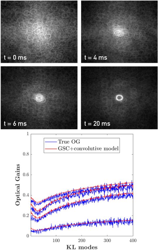
A&A 649, A70 (2021)

                                                                              We used the scalar product presented in Chambouleyron
                                                                          et al. (2020) to calculate the diagonal components of this matrix,
                                                                                   diag(MDt φ M)
                                                                          T Dφ =                     .                                    (6)
                                                                                    diag(M t M)
                                                                              Several approaches to practically compute this matrix can
                                                                          be found in the literature. They can be split into two categories:
                                                                          those that are invasive for the science path, consisting of send-
Fig. 1. Sketch of the PyWFS response curve for a given mode φi . The      ing some probe modes to the DM to return to the OG (Esposito
push-pull method around a null-phase consists of computing the slope      et al. 2015, Deo et al. 2019a), and those that rely on the knowl-
of this curve at φi = 0.                                                  edge of the statistics of the residual phases through the telemetry
                                                                          data to estimate the OG (Chambouleyron et al. 2020). In all the
the linear response,                                                      proposed methods, the OG can be seen as an evaluation of a time-
                                                                          averaged loss of sensitivity of the sensor. Being able to accurately
          s(aφi ) − s(−aφi )                                              retrieve OG allows compensating for the sensitivity loss.
δs(φi ) =                    .                                (1)
                  2a
    The interaction matrix (also called Jacobian matrix) is then          2.2. LPVS approach
the collection of the slopes recorded for all modes,
M = (δs(φ1 ), . . . , δs(φi ), . . . , δs(φN )).                   (2)    As described by Eq. (4), the PyWFS outputs are affected by the
   In this linear framework, we can then link the measured                incoming phase. The time-averaged definition of the interaction
phase with the output of the PyWFS by the relation                        matrix MDφ , is limited to a statistical behaviour of the PyWFS,
                                                                          even though it has good properties. We propose a framework
s(φ) = M.φ.                                                        (3)    that addresses the non-linearities in real time, with an interac-
     This matrix computation formalism has interesting prop-              tion matrix that is updated at every frame. To do so, we first
erties that are required in the AO control loop. However, the             assumed that the diagonal hypothesis holds. Then, and inspired
PyWFS exhibits substantial non-linearities that make the equa-            by the automatic field domain, the PyWFS is now considered as
tion above only partially true. Mathematically, the deviation             an LPVS (Rugh & Shamma 2000): Its linear behaviour encoded
from linearity is expressed with the following inequality: s(aφi +        by the interaction matrix is modified at each frame according to
φ) , s(aφi ) + s(φ), where φ is a non-null given phase. When              the incoming phase. Under this framework, the new expression
working around φ, the slope of the linear response of the sensor          of the PyWFS output can be written as
is therefore modified,
                                                                          s(φ) = Mφ .φ ≈ M.T φ .φ,                                        (7)
            s(aφi + φ) − s(−aφi + φ)
δsφ (φi ) =
                       2a                                                 where T φ is the OG matrix for the given measured phase φ.
          , δs(φi ).                                           (4)        Assuming the diagonal approximation holds, we can extract T φ
                                                                          from the interaction matrix computed around φ,
    During AO observation, the sensor is working around a non-
null phase φ corresponding to the residual phase of the system.                  diag(Mφt M)
As a consequence of Eq. (4), the response of the system is mod-           Tφ =                   .                                        (8)
                                                                                   diag(M t M)
ified. Previous studies suggested updating the response slopes to
mitigate this effect by relying on two main concepts. The first               For a given system, repeating this operation on a set of dif-
concept is the stationarity of the residual phases (Rigaut et al.         ferent phases will eventually lead to the time-averaged definition
1998). For a given system and fixed parameters (seeing, noise,            of the OG matrix,
etc.), we can compute an averaged response slope for each mode.
It has been proven (Fauvarque et al. 2019) that under this sta-           hT φ i = T Dφ .                                                 (9)
tionarity hypothesis, the averaged response slope depends on the
behaviour of the statistical residual phases through their struc-              To illustrate the difference between the time-averaged
ture function (Dφ ), hδsφ(φi ) i = δsDφ (φi ).The second concept is the   response and a single realisation, we performed the simula-
diagonal approximation (Korkiakoski et al. 2008). This approx-            tion presented in Fig. 2. These simulations were made with
imation implies considering no cross-talk between the modes,              parameters consistent with an 8m telescope and for two seeing
which means that the response slopes are only modified by a               conditions. All results showed in this paper rely on end-to-
scalar value for each mode. This value is known as the OG. We             end simulations performed with the OOMAO Matlab toolbox
then have δsDφ (φi ) = tDi
                             .δs(φi ), where tDi
                                                   is the OG associated   (Conan & Correia 2014). The exact conditions and parameters
                           φ                     φ
                                                                          are summarised in Table 1. In the simulation, we can compute
with the mode i for a given residual phase perturbation statistics        the exact PyWFS response by freezing the entrance phase and
characterised by the structure function Dφ . In this approxima-           performing a calibration process around this working point. We
tion, the shape of the response is left unchanged.                        therefore computed T φ for 1000 residual phase realisations, and
    Finally, the interaction matrix is updated by multiplying by a        show the OG variability for two seeing conditions in Fig. 2. This
diagonal matrix T Dφ called the OG matrix, whose diagonal com-            represents an optimistic context where the Fried parameter r0
              i
ponents are tD  φ
                  ,                                                       is fixed through the complete simulation. By estimating the T φ
s(φ) = hMφ i.φ                                                            with a time-averaging strategy, the errors on the OG correspond-
                                                                          ing to a given residual phase can reach more than some dozen
     = MDφ .φ                                                             percent (OG exhibiting a maximum deviation from the averaged
      ≈ M.T Dφ .φ.                                                 (5)    value are highlighted. This result illustrates the potential gain

A70, page 2 of 7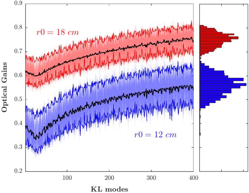
V. Chambouleyron et al.: Focal-plane-assisted pyramid wavefront sensor: Enabling frame-by-frame optical gain tracking

                                                                                   Fig. 3. Gain scheduling camera: A focal plane camera that records the
                                                                                   intensities of the modulated EM field with the same pyramid field of
                                                                                   view. This operation requires using part of the flux from the pyramid
                                                                                   path.

Fig. 2. Variability of closed-loop OG. For given system parameters we
compute T φ for 1 000 phase realisations in two seeing configurations:
r0 = 18 cm and r0 = 12 cm. The variability of the frame-by-frame
OG is shown in the histogram in the right panel and by the highlighted
extreme OG curves for each r0 case.

Table 1. Simulation parameters.

 Resolution                         80 pixels in telescope diameter
                                                                                   Fig. 4. Left: gain scheduling camera image for a flat wavefront. The
 Telescope                         D = 8 m – no central obstruction                white circle is produced by the tip-tilt modulation of the pyramid signal.
 Atmosphere                           Von-Karman PSD – 3 layers                    Right: gain scheduling camera image for a given closed-loop residual
 Deformable mirror   Generating atmospheric Karhunen-Loéve (KL) basis: 400 modes   phase.
 Sensing Path                       λ = 550 nm – 40 subpupils in D

                                                                                   the circle of modulation. This is illustrated in Fig. 4, where the
                                                                                   modulation circle is shown on the left, and the replicas of this
of performing a frame-by-frame estimation of the OG instead
                                                                                   modulation circle by the focal plane speckles are shown on the
of a time-averaged one. In the next section, a practical means
                                                                                   right. By denoting Ωφ the GSC signal, we can therefore write
for performing this frame-by-frame gain-scheduling operation is
presented.                                                                         Ωφ = PSFφ ? ω,                                                       (10)
                                                                                   where ω is the modulation weighting function. This function can
3. Gain-scheduling camera                                                          be thought of as a map of the incoherent positions reached by the
                                                                                   EM field on the pyramid during one integration time of the WFS
3.1. Principle
                                                                                   camera. This function is thus a circle for the circularly modu-
Obtaining an estimate of the OG values (the diagonal of T φ )                      lated PyWFS (Fig. 5 right). Ωφ has to be understood as the effec-
requires obtaining additional information describing the work-                     tive modulation weighting function: The phase to be measured
ing point of the PyWFS at each moment, independently of the                        produces its own modulation, leading to PyWFS loss of sensi-
PyWFS measurements themselves. To this end, a specific sensor                      tivity, and the GSC is therefore a way to monitor this additional
called gain-scheduling camera (GSC) is implemented.                                modulation.
    Empirically, it is well known that the PyWFS sensitivity                            The next step is now to link this focal plane information
depends on the structure of the EM field when it reaches the                       with the PyWFS optical gains and merge the GSC and PyWFS
pyramid mask. For instance, the more this field is spread over                     signal in one final set of WFS outputs. In a previous work
the pyramid mask, the less sensitive the PyWFS. In addition,                       (Chambouleyron et al. 2020), we demonstrated that the con-
because sensitivity and dynamic range are opposing properties,                     volutive model of the PyWFS developed by Fauvarque et al.
a well-known technique used to increase the PyWFS dynamic                          (2019) can be used to predict the averaged OG if the statistical
range consists of modulating the EM field around the pyramid                       behaviour of the residual phases (through the knowledge of their
apex. In order to keep track of the sensor regime, we therefore                    structure function) is known. In Eq. (11) we recall the expression
suggest probing this EM field by acquiring a focal plane image                     of the PyWFS output in this convolutive framework,
synchronously with the Pyramid WFS data. This can be achieved
by placing a beam splitter before the pyramid mask and record-                     s(φ) = IR ? (I p φ),                                                 (11)
ing the signal with a focal plane camera that has the same field                   where IR is the impulse response of the sensor and the star
of view as the pyramid (Fig. 3).                                                   denotes the convolutive product. In the framework of the infinite
    In this configuration, the focal plane camera, hereafter called                pupil approximation, the impulse response around a flat wave-
the GSC, records the intensity of the modulated EM field seen                      front can be expressed through two quantities, the mask complex
by the pyramid. By using the same exposure time and frame                          function m and the modulation function ω (Fig. 5),
rate as the WFS camera, the signal observed is then an instanta-
neous AO-corrected point-spread function (PSF) convolved with                      IR = 2Im(b m?b
                                                                                            m(b ω)).                                                    (12)
                                                                                                                                           A70, page 3 of 7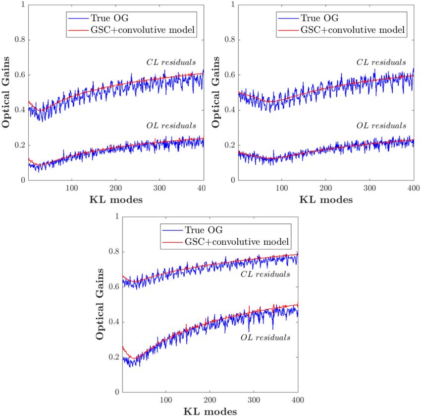
A&A 649, A70 (2021)

Fig. 5. Left: arg(m), the shape of the pyramid phase mask in the focal
plane. Right: ω, the modulation weighting function: Different positions
reached by the EM field during one integration time.

    We propose here to combine this model with the signal deliv-
ered by the GSC in order to compute the impulse response IRφ
of the PyWFS around each individual phase realisation. To do
this, we replaced ω by the GSC data as described in Eq. (13),

IRφ = 2Im(b m?Ω
          m(b cφ )).                                              (13)
                                                                          Fig. 6. OG estimation for given residual phases thanks to the GSC are
     This new way to compute the impulse response can be con-             compared with end-to-end simulation for different parameters (same
sidered as using the impulse response given for an infinite pupil         framework as in Fig. 2). OL: Open loop, and CL: closed-loop resid-
system (Eq. 12) for which we replaced the modulation weighting            ual phases. Left: r0 = 12 cm and rmod = 3λ/D. Middle: r0 = 12 cm and
function by the energy distribution at the focal plane, including         rmod = 5λ/D. Right: r0 = 18 cm and rmod = 3λ/D.
both the modulation and the residual phase.
     Now that we are able to compute IRφ at each frame, we can
estimate the OG matrix Teφ through the following computation              section is then to demonstrate that our GSC approach is only
of its diagonal components as described in Chambouleyron et al.           weakly affected by photon noise and therefore requires only a
(2020),                                                                   small number of photons while performing an accurate frame-
                                                                          by-frame OG estimation. To this end, we propose to inject noise
            hIRφ ? φi |IRcalib ? φi i                                     in the data delivered by the GSC and to probe the effect on the
t˜Di φ =                                 ,                        (14)
           hIRcalib ? φi |IRcalib ? φi i                                  OG estimation.
                                                                              We ran simulations with the same parameters as described
where IRcalib is the impulse response computed for the calibra-           above. The sensing path works around the central wavelength
tion state, most commonly for φ = 0 (Fig. 4, left).                       λc = 550 nm with the given bandwidth ∆λ = 90 nm and an ideal
                                                                          transmission of 100%. The exposure time of the GSC is 2 mil-
3.2. Accuracy of the estimation                                           liseconds (frame rate of the loop), and 10% of the photons are
                                                                          used by the GSC camera. The GSC pixel size corresponds to
It is now possible to test the accuracy of our estimator by com-          Shannon sampling of the diffraction-limited PSF. In this given
paring Teφ and T φ . To do this, we computed the true T φ through         configuration, the data recorded by the GSC for a given closed-
end-to-end simulations by proceeding through the ideal way                loop residual phase (r0 = 14 cm, rmod = 3 λ/D) are presented
described in section above: An interaction matrix was computed            in Fig. 7 (top) for (a.) a noise-free system, (b.) a guide-star mag-
around each given residual phase, from which the OG matrix                nitude equal to 8 (c.) a guide-star magnitude equal to 10, and
was derived (Eq. 8). This provides the ground truth to which the          (d.) a guide-star magnitude equal to 12. For these three noise
gains estimated with the GSC are compared.                                configurations (mag = 8, 10, and 12), we estimated the OG for
     First results are shown in Fig. 6 for different seeing and           500 realisations of the noise. The results are given Fig. 7 (bottom
modulation conditions. As illustrated in Fig. 6, the real and esti-       part). The introduction of noise leads to an increased OG estima-
mated OG agree well, demonstrating the accuracy of the pro-               tion error, which logically scales with the signal-to-noise ratio
                                                                                                √
posed method.                                                             (S/N) according to nph . However, the GSC approach also still
     For the parameters used in our simulations, the estimation           performs a satisfactory OG estimation even for low-magnitude
remains accurate regardless of whether we are in open loop or             guide stars. For even fainter guide stars, the noise effect might
closed loop. The ripples seen in the ground-truth OG curves are           be mitigated by integrating the GSC data over several frames. A
smoothed in the convolutive framework. The convolutive prod-              trade-off between noise propagation and OG error would then be
uct given in Eq. (11) tends to smooth the output of the PyWFS             required.
even when the impulse response is computed around a non-                      These results are crucial because they demonstrate that the
zero phase. Figure 6 also shows a slight deviation for low-order          GSC can be used with only a small fraction of WFS photons,
modes for a low-modulation regime and a strong entrance phase             leading to a limited repercussion on the S/N on the PyWFS. We
(open loop here).                                                         therefore have a way to estimate the OG, and to some extent
                                                                          increase the linearity of the sensor while having a reduced effect
                                                                          on its sensitivity.
3.3. Robustness to noise
The GSC has shown to be a reliable way to perform a fast                  3.4. GSC spatial sampling
OG tracking, but it requires using a fraction of the photons
available in the sensing path. This inevitably competes with the          Another aspect is the sampling of the GSC detector with
gain of sensitivity provided by the PyWFS. The goal of this               respect to the modulated PSF. If an under-sampling could be
A70, page 4 of 7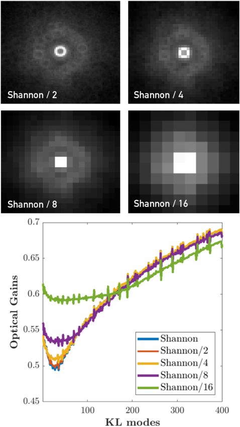
V. Chambouleyron et al.: Focal-plane-assisted pyramid wavefront sensor: Enabling frame-by-frame optical gain tracking

                                                                         Fig. 8. Effect of the GSC sampling on OG estimate for a given closed-
                                                                         loop residual phase (r0 = 14 cm, rmod = 3). Top: images delivered by
                                                                         the GSC with different samplings. Bottom: effect on the OG estimate.

                                                                         limited size allows for the use of low-readout noise cameras such
                                                                         as GSC, and remaining in a photon-noise limited regime.
                                                                             To conclude this section, we have shown that it is possible
                                                                         to perform OG fast-tracking by using an image of the modu-
Fig. 7. Top: closed-loop GSC images for different entrance fluxes. In    lated EM field at the focal plane. Our method uses a so-called
the chosen configuration, the exposure time is 2 ms, and we collect      GSC providing non-biased information on the working point of
10% of the photons in the sensing path. a: infinite number of photons.   the PyWFS, and the subsequent OG estimate using a convolu-
b: Guide-star magnitude = 8 (nph = 55 000 on the GSC). c: Guide-star     tive model. We demonstrated that the GSC can work with a lim-
magnitude = 10 (nph = 9000 on the GSC). d: Guide-star magnitude = 12
(nph = 1400 on the GSC). Bottom: OG estimate for the noise-free sys-
                                                                         ited number of photons and pixels, which makes the practical
tem compared with the three noisy configurations.                        implementation fully feasible. The next section is dedicated to
                                                                         quantifying the performance benefits of OG fast tracking with
                                                                         the GSC.
considered, it would reduce the number of pixels required by
the GSC, and consequently reduce the practical implementation
complexity. To test this, we ran our algorithm for various sam-          4. Application to specific AO control issues:
plings of the GSC in order to see the effect on the OG estimation.          Bootstrapping and NCPA handling
The results for a given closed-loop residual phase (r0 = 14 cm,          As shown in the previous sections, the GSC allows tracking the
rmod = 3) are given in Fig. 8. The sampling of the PSF can go            PyWFS OG frame by frame and compensating for these non-
below the Shannon sampling (2 pixels per λ/D) without signif-            linearities. We illustrate here two possible situations in which the
icant effect on the estimate. This result depends on the modula-         GSC can significantly improve the performance: bootstrapping
tion radius rmod used, and we note that the OG estimate is not           and NCPA handling.
affected as long as the pixel size dpx satisfies the Shannon crite-
rion for the modulation radius,
                                                                         4.1. Bootstrapping
dpx ≤ rmod /2.                                                   (15)
                                                                         During the AO loop bootstrap, the PyWFS faces large ampli-
When this criterion is not respected, the undersampled modula-           tude wavefronts (due to uncorrected turbulence), leading to
tion circle is seen as a disc (Fig. 8), which affects the OG esti-       significant non-linearities that may prevent the loop from clos-
mate for low-order modes.                                                ing. Therefore this step is critical because it corresponds to the
    As a concrete example, a PyWFS for the Extremely Large               moment at which the OGs are the most important. Monitoring
Telescope (ELT) working at λ = 800 nm with a field of view of            them frame by frame in order to update the reconstructor helps
2 arcsecs and with a sampling of Shannon/4 on the GSC would              closing the AO loop. Because of the timescales involved in the
require a GSC camera with no more than 250 × 250 px. This                AO loop bootstrap, this problem cannot be tackled by other OG
                                                                                                                             A70, page 5 of 7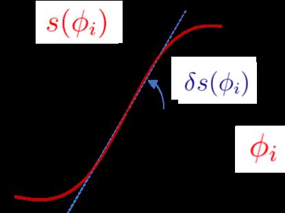
A&A 649, A70 (2021)

                                                                        Fig. 10. OG-compensated bootstrap vs. OG-uncompensated bootstrap.

                                                                        4.2. NCPA handling
                                                                        Handling NCPA is emerging as one of the main issues due to
                                                                        PyWFS OG, as was demonstrated for instance on the Large
                                                                        Binocular Telescope (Esposito et al. 2015). How to handle this
                                                                        issue while having an accurate OG estimation was discussed
                                                                        in a previous paper (Chambouleyron et al. 2020). We briefly
                                                                        recall the main problem. The NCPA reference measurements
                                                                        are recorded around a diffraction-limited PSF and need to be re-
Fig. 9. Bootstrapping with the help of the GSC. Top: images delivered
                                                                        scaled by the OG while working on sky: s(φNCPA ) ←- sφ (φNCPA ).
by the GSC at a time. t = 0 represents the beginning of the servo-      To compute sφ (φNCPA ), we need to have estimate T φ ,
loop. The frame rate of the AO loop is still fixed at 2 ms with r0 =    sφ (φNCPA ) = Mφ .φNCPA
12 cm and rmod = 3λ/D. Bottom: OG estimate during bootstrapping for
the corresponding images on the left. Lower OG corresponds to higher                = Mcalib .T φ .φNCPA .                           (17)
residuals on the pyramid, hence to the first frames of loop closure.
                                                                             We show here the results of a simulation in which we used
                                                                        the GSC to handle NCPA in the AO loop. We retained the same
handling techniques that were previously studied in the litera-         simulations parameters as before (caption of Fig. 2). The PyWFS
ture. The best solutions already proposed endures necessarily           modulation radius was rmod = 3 λ/D and r0 = 14 cm. The
delays of a few frames (Deo et al. 2019b). Here, we can estimate        interaction matrix was computed around a flat wavefront. We
the OG corresponding to the current measurement frame: This             injected 200 nm rms of NCPA into our system, distributed with
is an unprecedented feature. We show different images deliv-            a f −2 power law on the first 25 KL modes (except for tip-tilt and
ered by the GSC during the bootstrap operation in Fig. 9. The           focus). In this configuration and for a flat wavefront in the sci-
corresponding estimated OGs are also plotted, compared with             ence path (H band), the PSF in the wavefront sensing path (V
the end-to-end computation giving the true OG values. While             band) is given in Fig. 11a and the signal ΩφNCPA seen by the GSC
the loop is closing, the OG varies from low values to higher            is shown in Fig. 11b.
values, indicating that the residual phases reaching the PyWFS               We then proceeded in the following way: We closed the loop
decrease: The loop is closing, and the DM is starting to correct        on the turbulence, and after 5 s of closed-loop operation, the
the atmospheric aberrations. Our technique performs a precise           NCPA was added to the system. These NCPAs were then han-
OG follow-up during all the steps of the process, at the frame          dled with different configurations, and the results were compared
rate of the loop.                                                       with the NCPA-free case. Figure 12 illustrates the results. The
     We can use our frame by frame OG estimation to update the          main conclusions from Fig. 12 are listed below.
reconstructor while the loop is closing. The reconstructor is the        1. When the NCPA is not compensated for (orange plot), the
pseudo-inverse of the interaction matrix. We can therefore relate            loop converges toward a flat wavefront in the sensing path.
it to the OG matrix and the calibration interaction matrix through           This induces a high loss of Strehl ratio (SR) in the science
the following formula:                                                       path, corresponding to the NCPA.
                                                                         2. When a reference map s(φNCPA ) in the PyWFS measure-
                                                                             ment is used without updating it by the OG, this leads to
Mφ† = T φ−1 Mcalib
             †
                   .                                            (16)         a divergence of the loop (so-called NCPA catastrophe, yel-
                                                                             low plot). This can be explained by the fact that because of
    By doing so, we show that it is possible to close the loop               the OG, the PyWFS introduces too much NCPA, creating
faster. A simulation example is presented by comparing a loop                an even stronger aberrated wavefront. This aberrated wave-
bootstrap with and without OG compensation by the GSC cam-                   front increases the OG in the next frame, which continues to
era (Fig. 10). This example, with a limited benefit in practice,             increase the aberration, and so on. This quickly causes the
shows how a fast OG tracking combined with the corresponding                 loop to diverge.
update of the reconstructor can be applied to mitigate all types         3. When the reference map is compensated for by the time-
of short-timescale residual variations, such as seeing bursts.               averaged OG computed in the first 5 s of the loop by a
A70, page 6 of 7
V. Chambouleyron et al.: Focal-plane-assisted pyramid wavefront sensor: Enabling frame-by-frame optical gain tracking
starting to consider other non-linear (second- or third-order
description) solutions, which goes beyond the computation
framework of a simple matrix.
5. Conclusion
The PyWFS is a complex optical device exhibiting strong non-
linearities. One way to deal with this behaviour while keeping
a matrix computation formalism is to consider the PyWFS as
a LPVS. To probe the sensing regime of this system at each
measurement, a gain scheduling loop needs to be implemented
that gives information on the sensor regime at every moment.
With this perspective, the OG compensation can be deployed on
a frame-by-frame basis. We provided here an innovative solu-
tion to this end: the GSC combined with a convolutive model.
As such, the PyWFS data synchronously merged on a frame-
Fig. 11. a: PSF on the pyramid apex when a flat wavefront is set in the by-frame basis with GSC data can be thought of as a single
science path. b: GSC signal when there are no residual phases and for WFS combining images from different light-propagation planes.
a flat wavefront in the science path. c: GSC signal during closed-loop
It therefore provides an efficient way to compensate for non-
around NCPA.
linearities at each AO loop frame without any delay, and it signif-
icantly improves the final performance of the AO loop in terms
of sensitivity and dynamic range as well as robustness. It also
allows unambiguously disentangling the effect of OG from the
full AO loop gain, which is a fundamental advantage for NCPA
compensation. The GSC solution has now to be implemented on
the AO facility bench LOOPS at the LAM for an experimental
demonstration (Janin-Potiron et al. 2019).
Acknowledgements. This work benefited from the support of the WOLF project
ANR-18-CE31-0018 of the French National Research Agency (ANR). It has also
been prepared as part of the activities of OPTICON H2020 (2017-2020) Work
Package 1 (Calibration and test tools for AO assisted E-ELT instruments). OPTI-
CON is supported by the Horizon 2020 Framework Programme of the European
Commission’s (Grant number 730890). Authors are acknowledging the support
by the Action Spécifique Haute Résolution Angulaire (ASHRA) of CNRS/INSU
co-funded by CNES. Vincent Chambouleyron PhD is co-funded by “Région
Sud” and ONERA, in collaboration with First Light Imaging. Finally, part of
this work is supported by the LabEx FOCUS ANR-11-LABX-0013.
Fig. 12. Strehl ratio for different cases of NCPA handling. In this sim-
ulation context, the case for which we compensate for NCPA without References
scaling by the OG leads to a diverging loop. Chambouleyron, V., Fauvarque, O., Janin-Potiron, P., et al. 2020, A&A, 644, A6
Conan, R., & Correia, C. 2014, Proc. SPIE Int. Soc. Opt. Eng., 9148, 91486C
Deo, V., Gendron, É., Rousset, G., et al. 2019a, A&A, 629, A107
long-exposure image of the GSC (purple plot), no NCPA Deo, V., Rozel, M., Bertrou-Cantou, A., et al. 2019b, Adaptive Optics for
catastrophe appears, and the final performance reaches an Extremely Large Telescopes conference, 6th edn. Québec, France
Esposito, S., & Riccardi, A. 2001, A&A, 369, L9
averaged SR of 82%. Esposito, S., Pinna, E., Puglisi, A., et al. 2015, Adaptive Optics for Extremely
4. When the reference map is compensated for by the OG com- Large Telescopes 4-Conference Proceedings, 1
puted at each frame, using the GSC camera (green plot), the Fauvarque, O., Janin-Potiron, P., Correia, C., et al. 2019, J. Opt. Soc. Am. A, 36,
final performance reaches an averaged SR of 86%. This solu- 1241
Fauvarque, O., Neichel, B., Fusco, T., Sauvage, J.-F., & Girault, O. 2016, Optica,
tion is better than the previous one because we monitor the 3, 1440
OG at each frame, and we also take the effect of the NCPA Guyon, O. 2005, ApJ, 629, 592
themselves on the OG into account. To illustrate this, we Janin-Potiron, P., Chambouleyron, V., Schatz, L., et al. 2019, Adaptive Optics
show the GSC image for a given closed-loop residual when with Programmable Fourier-based Wavefront Sensors: a Spatial Light
the NCPA is compensated for in Fig. 11c. Modulator Approach to the LOOPS Testbed
Korkiakoski, V., Vérinaud, C., & Louarn, M. L. 2008, in Adaptive Optics
This study is a clear demonstration that our strategy can solve Systems, eds. N. Hubin, C. E. Max, & P. L. Wizinowich, Int. Soc. Opt.
the AO control issue due to PyWFS OG. It also shows that Photonics (SPIE), 7015, 1422
even if the OGs are compensated for on a frame-by-frame basis, Ragazzoni, R. 1996, J. Mod. Opt., 43, 289
the ultimate performance (without NCPA) cannot be reached. Rigaut, F. J., Veran, J. P., & Lai, O. 1998, in Adaptive Optical System
Technologies, eds. D. Bonaccini, & R. K. Tyson, Int. Soc. Opt. Photonics
This limitation is mainly due to the LPVS approach, which is (SPIE), 3353, 1038
characterized by a linear description of the whole sensing prob- Rugh, W. J., & Shamma, J. S. 2000, Automatica, 36, 1401
lem. Improving the performance further would probably mean Vérinaud, C. 2004, Opt. Commun., 233, 27
A70, page 7 of 7You can also read