Digital servo power amplifi er
←
→
Page content transcription
If your browser does not render page correctly, please read the page content below
Tuning guide
H-1000-5246-03-A

Digital servo power amplifier
© 2003 - 2006 Renishaw plc. All rights reserved.

This document may not be copied or reproduced in whole or in part, or
transferred to any other media or language, by any means, without the prior
written permission of Renishaw.

The publication of material within this document does not imply freedom from
the patent rights of Renishaw plc.

Disclaimer

Considerable effort has been made to ensure that the contents of this
document are free from inaccuracies and omissions. However, Renishaw
makes no warranties with respect to the contents of this document and
specifically disclaims any implied warranties. Renishaw reserves the right to
make changes to this document and to the product described herein without
obligation to notify any person of such changes.

Trademarks

RENISHAW® and the probe emblem used in the RENISHAW logo are
registered trademarks of Renishaw plc in the UK and other countries.

apply innovation is a trademark of Renishaw plc.

All brand names and product names used in this document are trade names,
service marks, trademarks, or registered trademarks of their respective owners.

Renishaw part no: H-1000-5246-03-A
Issued: 03 2006
Digital servo power amplifier

        tuning guide

     SPA2 and SPAlite
2             Care of equipment

Care of equipment
Renishaw probes and associated systems are precision tools used for obtaining precise measurements
and must therefore be treated with care.

Changes to Renishaw products
Renishaw reserves the right to improve, change or modify its hardware or software without incurring any
obligations to make changes to Renishaw equipment previously sold.

Warranty
Renishaw plc warrants its equipment for a limited period (as set out in our Standard Terms and Conditions
of Sale) provided that it is installed exactly as defined in associated Renishaw documentation.

Prior consent must be obtained from Renishaw if non-Renishaw equipment (e.g. interfaces and/or cabling)
is to be used or substituted. Failure to comply with this will invalidate the Renishaw warranty.

Claims under warranty must be made from authorised service centres only, which may be advised by the
supplier or distributor.

Trademarks
Windows 98, Windows XP, Windows 2000 and Windows NT are registered tradenames of the Microsoft
Corporation.

All trademarks and tradenames are acknowledged.

References and associated documents
It is recommended that the following documentation is referenced to when installing the UCC.

Renishaw documents
Documentation supplied on Renishaw UCC software CD.

Document number          Title

H-1000-5057        UCC controller programmer’s guide

H-1000-5058        UCC Renicis user’s guide

H-1000-5223        UCC2 installation guide

H-1000-5234        SPA2 installation guide

H-1000-5227        SPA1 servo tuning guide
Contents                            3

                                                                    Contents
1 Introduction..........................................................................................................................................5
2 Digital SPA commissioning sequence .................................................................................................6
         2.1       Initial machine ini file creation ..............................................................................................6
                   2.1.1         Common parameters ............................................................................................6
                   2.1.2         SPAlite only ..........................................................................................................7
                   2.1.3         SPA2 only .............................................................................................................8
                   2.1.4         Machine and move configuration..........................................................................9
         2.2       Renicis sequence...............................................................................................................10
                   2.2.1         Initial steps..........................................................................................................10
                   2.2.2         SPA2 configuration screen .................................................................................11
                   2.2.3         Check readheads................................................................................................12
                   2.2.4         Configure motor and feedback polarity...............................................................12
                   2.2.5         Current – loop tuning ..........................................................................................12
                   2.2.6         Velocity loop tuning with motor tachometer feedback ........................................15
                   2.2.7         Velocity loop tuning with motor encoder feedback .............................................18
                   2.2.8         Adjustment of scaling factor, proportional, integral and derivative gains............21
         2.3       Position loop tuning............................................................................................................23
                   2.3.1         Setting the uncompensated gain ........................................................................23
                   2.3.2         Applying acceleration feedback ..........................................................................25
         2.4       Servo tuning .......................................................................................................................27
                   2.4.1         Servo tuning test.................................................................................................27
                   2.4.2         Servo tuning adjustment .....................................................................................29
                   2.4.3         Applying velocity feed-forward............................................................................30
                   2.4.4         Scanning tuning procedure.................................................................................31
         2.5       Torque mode tuning procedure ..........................................................................................32
                   2.5.1         Initial steps..........................................................................................................32
                   2.5.2         SPA2 configuration screen .................................................................................32
                   2.5.3         Velocity Loop tuning ...........................................................................................33
                   2.5.4         Position loop tuning ............................................................................................36

3 Rotary table tuning procedure ...........................................................................................................39
         3.1       Overview ............................................................................................................................39
                   3.1.1         Initial settings ......................................................................................................39
         3.2       Tuning ................................................................................................................................40
                   3.2.1         Velocity loop tuning.............................................................................................40
                   3.2.2         Position loop tuning ............................................................................................41

4 Definitions..........................................................................................................................................43
         4.1       Uncompensated gain .........................................................................................................43
         4.2       Acceleration feedback........................................................................................................43
         4.3       Dynamic integrator .............................................................................................................43
         4.4       Velocity feed-forward .........................................................................................................43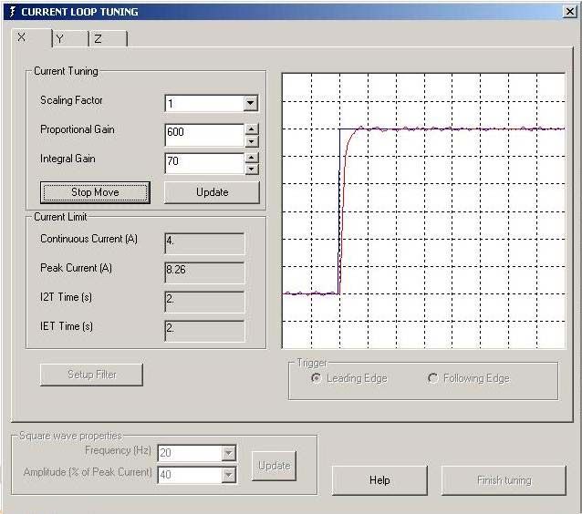
4                  Contents

         4.5      I2t Time .............................................................................................................................. 44
         4.6      IET Time............................................................................................................................ 44
         4.7      Overshoot (per axis).......................................................................................................... 44
         4.8      Following error (per axis, already existing)........................................................................ 44
         4.9      Steady state error (per axis).............................................................................................. 44
         4.10 Settling time (per axis)....................................................................................................... 44
         4.11 Tunnelling error (for the 3D move) .................................................................................... 45
5 Appendices ....................................................................................................................................... 46
         5.1      Current and velocity loop filters ......................................................................................... 46
                  5.1.1          Current filter ....................................................................................................... 46
                  5.1.2          Acceleration filter ............................................................................................... 46
                  5.1.3          Forward filter 1 and Forward filter 2 ................................................................... 47
                  5.1.4          Derative filter...................................................................................................... 47
                  5.1.5          Tacho filter ......................................................................................................... 47
         5.2      Glossary of terms .............................................................................................................. 48
6 Revision history ................................................................................................................................ 49
         6.1      What’s new in release 01-A............................................................................................... 49
         6.2      What’s new in release 02-A............................................................................................... 49
         6.3      What’s new in release 03-A............................................................................................... 49
Introduction               5

1     Introduction
The object of this digital servo power amplifier tuning guide is to provide a user-friendly publication to
assist in the task of setting up the servo response of the CMM when fitted with either a SPA2 or SPAlite
servo power amplifier. Used in conjunction with Renishaw’s “RENICIS” installation / fault finding software,
this document should enable a competent technician to set up a CMM either at the assembly plant or
on-site.

The Renishaw controller family of products has a powerful range of control elements to assist with tuning
(attaining the required performance) the CMM system, including; gain control, lead and lag filters, dynamic
integrator, acceleration feedback and velocity feed-forward.

The theories behind optimal tuning of control system are lengthy and complex, so we have tried in this
issue to simplify the set-up steps that deal with servo-optimisation. A set of performance indices is
available to allow checking of the machine tuning at any time and a report can be generated.
6             Digital SPA commissioning sequence

2       Digital SPA commissioning sequence
The following section outlines the recommended procedure to commission either the SPA2 or SPAlite
digital servo power amplifiers.

This procedure assumes that the system being installed is a new installation and little information is known
about the machine’s servo system characteristics.

2.1         Initial machine ini file creation
Using Renicis create a new machine ini file, the following critical parameters must be correctly specified
for the initial installation process.

NOTE: Most of the default parameters specified in the machine configuration file can remain as default.

2.1.1       Common parameters

        MachineDescription section
                  Make                                     This should be the make of machine
                  Model                                    This should be the model of the machine

        Miscellaneous section
                  LogFilePath                              This should be a valid file path

        MachineConfiguration section
                  ProbeHeadType                            Probe head type fitted to the machine
                  XscaleIncrement                          Resolution of the X axis scale in mm
                  YscaleIncrement                          Resolution of the Y axis scale in mm
                  ZscaleIncrement                          Resolution of the Z axis scale in mm
                  Xtravel                                  Distance of machine X axis travel in mm
                  Ytravel                                  Distance of machine Y axis travel in mm
                  Ztravel                                  Distance of machine Z axis travel in mm

        MoveConfiguration section
              *   MaximumMoveSpeed                         Maximum move speed of the CMM in mm/s
                  MaximumMoveAcceleration                  Maximum move acceleration of the CMM in
                                                           mm/s/s

        *     See section 2.1.4 for an explanation of this parameter and its importance.

        TORQUEMODE (if used)
                  ControlMode                              Torque mode is enabled or not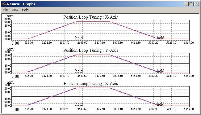
Digital SPA commissioning sequence      7

        MachineIOLogic
               AmpifierOK                    Logic level active high or low
               CMMdeclutch                   Logic level active high or low
               ESTOPtripped                  Logic level active high or low
               AirPressureLow                Logic level active high or low
               ZaxisCrash                    Logic level active high or low
               MotorsEngaged                 Logic level active high or low
               OuterLimitXPositive           Logic level active high or low
               OuterLimitXNegative           Logic level active high or low
               OuterLimitYPositive           Logic level active high or low
               OuterLimitYNegative           Logic level active high or low
               OuterLimitZPositive           Logic level active high or low
               OuterLimitZNegative           Logic level active high or low
               InnerLimitXPositive           Logic level active high or low
               InnerLimitXNegative           Logic level active high or low
               InnerLimitYPositive           Logic level active high or low
               InnerLimitYNegative           Logic level active high or low
               InnerLimitZPositive           Logic level active high or low
               InnerLimitZNegative           Logic level active high or low
               OuterLimitY2Positive          Logic level active high or low
               OuterLimitY2Negative          Logic level active high or low
               InnerLimitY2Positive          Logic level active high or low
               InnerLimitY2Negative          Logic level active high or low

2.1.2     SPAlite only

        SPAX
               ChannelNumber                 =0
               SPAType                       = SPAlite

        SPAY
               ChannelNumber                 =1
               SPAType                       = SPAlite

        SPAZ
               ChannelNumber                 =2
               SPAType                       = SPAlite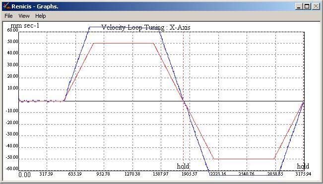
8              Digital SPA commissioning sequence

2.1.3       SPA2 only

        Dual Y section (if fitted)
                  DualAxisScaleIncrement                  Resolution of the dual axis scale in mm
                  WhichAxisDual                           Which axis is the dual axis
                  DualDriveEnable                         Is the dual drive switched on
                  ScaleInputLocation                      UCC input location address
                  DriveOutputLocation                     UCC output location address

        RotaryTable (if fitted)
                  MeasurementUnits                        Units of increment for the rotary table
                  WscaleIncrement                         Resolution of the W axis scale
                  WmaximumMoveSpeed                       Maximum move speed of the rotary table
                  WmaximumMoveAcceleration                Maximum move acceleration of the rotary table

        Torque mode (used where motors with no tachimeter or encode feedback are fitted)
                  Control mode                            = 1 if enabling torque mode
                  Feedback gain (X, Y and Z)              = (10 / MaximumMoveSpeed)
                  Refer to section 2.5.1.

        SPAX
                  ChannelNumber                           = 0*
                  SPAType                                 = SPA2

        SPAY
                  ChannelNumber                           = 1*
                  SPAType                                 = SPA2

        SPAZ
                  ChannelNumber                           = 2*
                  SPAType                                 = SPA2

        SPAW (if fitted)
                  ChannelNumber                           The SPA2 output channel number*

        SPADUAL (if fitted)
                  ChannelNumber                           The SPA2 output channel number*

        SPAConfiguration
                  SPA2ConfigurationFilePath               A valid file path if a SPA2 configuration file
                                                          ,otherwise leave blank.

        *      The SPA2 channel number is the output channel that the motor is connected to on the SPA2.
               Typically between 0 and 3, but can be between 0 and 7).
!
Digital SPA commissioning sequence 9
2.1.4 Machine and move configuration
This is a very important part of the machine set-up where all the physical and motion properties are
defined.
CAUTION: Particular care is needed in specifying the maximum move speed and acceleration
! since this defines the velocity gain of the remainder of the CMM servo system (the motors, the
tacho-generators (if fitted) and the drive gearing).
The “MaximumMoveSpeed” is a theoretical speed which corresponds to a maximum demand being
applied to the servo power amplifier. To control a specified speed, we apply a margin about that speed to
effect control. This is set to 20%. This means that the actual maximum move speed is 80% of the
“MaximumMoveSpeed” specified in the machine configuration file i.e. if you set “MaximumMoveSpeed” to
500 mm/s the maximum move speed you can request is 400 mm/s.
If maximum move speed is altered after the CMM has been commissioned (with no change in the CMM
hardware), two problems will become apparent: -
Problem 1
All machine speeds will be altered. e.g. if the maximum move speed value is halved, this implies that the
full 10 V motor command will now produce only half the previous speed. The controller will therefore
compensate by sending speed commands to the motors, which are twice the original values to get the
same target machine speeds. This will result in much faster moves than intended, with probably “over-
speed” and “overdriven” faults being produced.
NOTE: The machine speed in a command (move or scan) is limited to only 80% of the maximum move
speed to ensure servo control at all times.
Problem 2
If the machine’s performance characteristics change then some of the settings will become invalid. The
machine will need to be re-tuned.10 Digital SPA commissioning sequence
2.2 Renicis sequence
2.2.1 Initial steps
1. Start the commissioning process by ensuring the step icon on the toolbar is not indented and then
click on the GO icon on the toolbar, as shown in the figure 1 below:
Figure 1
2. The Renicis commissioning step list will now be displayed within a window that will open on the
desktop, as shown in the figure 2 below:
Figure 2
3. Highlight the Welcome step within the list and then click on the GoToStep button to start the
commissioning process.
4. Proceed through the following Renicis steps following the instructions:
• Welcome
• Connector and interface details
• Test link
• Emergency stop
• Other safety matters
• SPA2 configuration overview
5. If problems are experienced with any of the above steps, refer to the Renicis user guide (Renishaw
part number H-1000-5058) or UCC2 installation guide (Renishaw part number H-1000-5223).Digital SPA commissioning sequence 11
2.2.2 SPA2 configuration screen
For torque mode configuration please refer to section 2.5.2.
1. At this step, the following window will appear with the X axis screen presented (see figure 3 below):
Figure 3
2. Under VBus selection the bus voltage should be set to 60 V for a SPA2 installation and 48 V for a
SPAlite installation.
3. Select the correct motor and motor feedback type for the installation.
4. Enter the maximum motor voltage for the motor connected to the axis of the installation. Typically,
this is stamped on the body of the motor.
5. Select the nearest peak motor current from the drop down list. Typically, this is stamped on the
body of the motor.
6. Enter the continuous motor current specification. Typically, this is about 50% of the peak motor
current, but can sometimes be found on the body of the motor.
7. It is recommended that the I2T and IET time values are left at the default value of 2 s (refer to
section 4 for more information).
8. Repeat steps 2 to 6 for the other machine axes.
NOTE: It is possible to have different specification motors for different axes.
9. When all axes are complete click ‘Finish’.12 Digital SPA commissioning sequence
2.2.3 Check readheads
Continue to ‘Check Read Heads’ Renicis step and perform the test as instructed on the screen display.
2.2.4 Configure motor and feedback polarity
NOTE: It is essential that the scale resolution and polarity for all machine axis have been checked and
are correct before performing this step (section 2.2.3 ‘Check readheads’)..
The configure motor and feedback polarity steps automatically check and configure the motor and
feedback polarity for the installation.
During these steps, an increasing percentage of the machine’s maximum current will be applied to each
motor in turn with the aim of moving the machine a minimum of 1 mm.
Using the axis scales as reference the motor and feedback polarities are then automatically configured.
The configuration is finally checked by the next Renicis step ‘close position loop’.
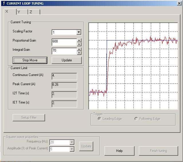
2.2.5 Current – loop tuning
In this section you are tuning the current-loop to ensure that:
a) The amplifier delivers the required current to the motors.
b) High frequencies are not introduced by the response being too sharp.
At this step the following screen will appear with the X axis active:
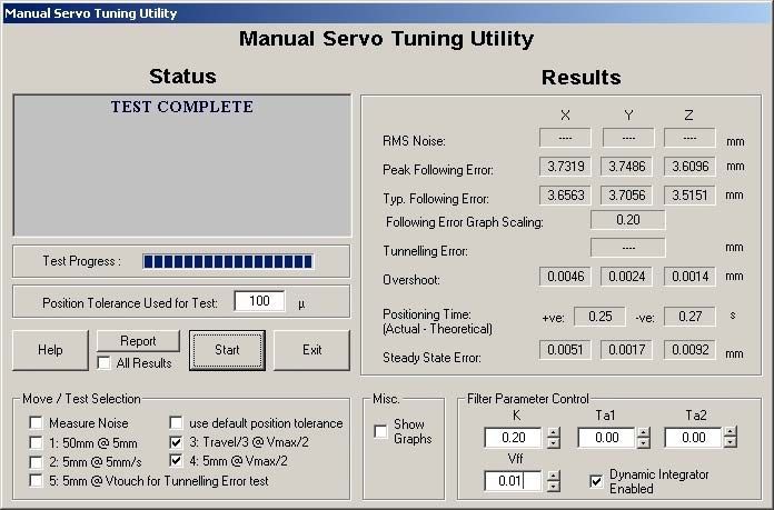
Figure 4Digital SPA commissioning sequence 13
1. Start the current loop tuning by clicking on the “Start move” button this will produce a waveform
something like that shown in the example on previous page.
2. Experience has shown that at this stage it is best not to tune this response to follow the square
wave precisely as shown in figure 4. It is better to achieve a response similar to the example shown
in figure 5 below with some initial rounding of the waveform. Adjust the proportional and integral
gain until a good response is obtained.
• Changes to the proportional and integral settings can be made using the up/down arrows located
to the side of the fields, otherwise the installer can type directly into the input box and then click
on the update button for this setting to be applied to the SPA2 system.
• The input boxes have a range from 0 to 32767, if values are required outside of this range then it
is possible to apply a multiplication factor to these values using the scaling factor.
• Increasing the scaling factor by one (i.e. 1 to 2 or 2 to 4) in the drop down box will effectively
double the value based on the previous scaling factor selection, reducing the scaling factor will
effectively half the value based on the previous scaling factor.
• The recommended method to be used during this process is firstly to increase the proportional
gain. If this is set too high, instability can be seen on the trace (high frequency oscillation). Next
increase the integral gain. This will have the effect of sharpening the response. However, if too
much integral gain is applied, an initial overshoot spike will become apparent.
Figure 5
3. Press “Stop Move” button and increase the amplitude in the square wave properties to 10%, the
machine response trace on the graph should change such that it follows the demand trace closer.
If overshoot is experienced as shown in figure 6, it will be necessary to re-tune the system to
remove this. Experience shows that typically increasing the proportional gain and/or reducing the
integral gain will permit the trace to match the demand closer.14 Digital SPA commissioning sequence
NOTE: Experience has shown that any overshoot, shown in figure 6, in the current loop tuning will reduce
the ability for the system to be optimised for scanning. An over damped response, as shown in figure 7,
should be achieved.
Figure 6
Figure 7
4. Repeat step 3, increasing the amplitude of the square wave (recommended steps 20%, 30%, 40%,
50%).
CAUTION: As the current loop is exciting the motor on the machine vibrations will become
! apparent, at the point of when the vibrations just start to introduce axis movement the amplitude of
the current should not be increased.Digital SPA commissioning sequence 15
NOTE: If there is a requirement for the amplitude to be increased past the 50% level then it is possible
that the IET error will cause the test to stop after its defined time period.
5. Click the stop button when complete.
6. Repeat step 1 to 5 for all other machine axis.
7. When all axis have been commissioned then clicking on the finish tuning button will save all the
parameters to the servo power amplifier and to the spa configuration file.
NOTE: Please refer to sections:
1. 2.2.6 for velocity loop tuning with motor tachometer feedback.
2. 2.2.7 for velocity loop tuning with motor encoder feedback.
3. 2.5.3 for torque mode tuning procedure.
2.2.6 Velocity loop tuning with motor tachometer feedback
NOTE: If your motors have encoder velocity feedback ignore this section and proceed to section 2.2.7.
This test moves the CMM forwards and backwards by the distance entered.
1. It is recommended that initially the tests are completed on individual axes, the X axis is selected by
deselecting the Y and Z axis check boxes.
2. Run the test using the default values to start with by clicking the Go button. Check the operate
continuously box to keep the machine moving, otherwise the machine will stop after one cycle.
NOTE: If the machine is unstable, it is recommended that the scaling factor is reduced by 1 step until you
have stability and can continue with the tests.
Increasing the acceleration value for this test will give a sharper square wave stimulus to the machine.16 Digital SPA commissioning sequence
The test will not change the maximum acceleration value stored in the UCC Configuration File.
Figure 8
NOTE: If you use the up/down arrows on this screen the new values are applied immediately. If you type
in the new values you have to click on the update button before the new value is applied. If the value is in
red type it has not been applied.
If the machine response amplitude does not match the demand you could get the following message:
Figure 9
Check the machine is still in the centre of its operating range, move it if necessary, click on the OK button,
click on the reset data button, then adjust the gain setting and continue the test by clicking on GO.
3. The initial adjustment is to set the tacho velocity feedback gain, using the up / down arrows or by
entering the value and clicking on update, to adjust the values until the amplitude of the plots are
matched. Figure 10 shows a graph plot were the tacho velocity feedback gain is set too high.Digital SPA commissioning sequence 17
NOTE: Decreasing the value in this box will have the effect of increasing the amplitude of the
machine speed.
Figure 10
If the gain is excessive, when setting the tacho feedback, then the following screen will be displayed
during the test.
Figure 11
If it appears you will need to click OK, click the Reset Datum button to zero the counters, adjust the
gain setting, then click on the Go button to start the test again.
4. The response of the servo system should now be set up for this axis, proceed to section 2.2.8.18 Digital SPA commissioning sequence
2.2.7 Velocity loop tuning with motor encoder feedback
NOTE: This section covers tuning of motors with encoder feedback. If you have tacho motors then the
set up will have been covered in section 2.2.6.
This test moves the CMM forwards and backwards by the distance entered.
Figure 12
NOTE: If you use the up/down arrows on this screen, the new values are applied immediately. If you type
in the new values you have to click on the update button before the new value is applied. If the value is in
red, it has not been applied.
1. It is recommended that initially the tests are completed on individual axes, the X axis is selected by
deselecting the Y and Z axis check boxes.
2. Before the test is started the encoder gain for the axis under test should be calculated such that the
machine moves close to the specified speed, the formula for calculating this is:
32767
Encoder gain =
(4*Encoder resolution (pulses/mm of axis travel )) x Max move speed (mm/s) x 0.0001
Enter this value into the “Encoder Velocity Feedback Gain” box. This value need not be accurate,
one significant figure is sufficient.Digital SPA commissioning sequence 19
3. When using an encoder as a velocity feedback device, it is normally necessary to include a filter.
This is required because the encoder has a finite resolution with step changes and you are
differentiating a digital signal into an analogue one. As a default for all encoder based feedback
systems a 500 Hz bandwidth low pass filter is applied to the tacho feedback. If it is necessary to
modify this setting, please follow the procedure listed below. Normally a 500 Hz bandwidth filter is
sufficient but if the encoder is low in resolution, it may be necessary to increase the filtering by
reducing the filter bandwidth.
Click on the “Setup filter” button located the following screen will open:
Figure 13
Enter a value of between 200 and 500 Hz (default = 500) into the “Auto Make Cut Off Freq” input box.
Right hand mouse click on the tacho filter box to open the filter type option screen and then click on the
“make 2nd order BW LP” to make a second order bandwidth low pass filter, as shown below.
Figure 14
Click on the DONE button to close the screen.
For details of where the filters are applied in the current loop please refer to section 5.20 Digital SPA commissioning sequence
4. Start the test, using the default values, by clicking the Go button. Check the operate continuously
box to keep the machine moving, otherwise the machine will stop after one cycle.
NOTE: If the machine is unstable, it is recommended that the scaling factor is reduced by 1 step
until you have stability and can continue with the tests.
Increasing the acceleration value for this test will give a sharper square wave stimulus to the
machine. The test will not change the maximum acceleration value stored in the UCCConfiguration
File.
5. The initial adjustment is to set the encoder velocity feedback gain, this can be done using the up /
down arrows or by entering the value and clicking on update, to adjust the values until the amplitude
of the plots are matched. Figure 15 shows a graph plot where the encoder velocity feedback gain is
set too low.
NOTE: Decreasing the value in this box will have the effect of increasing the amplitude of the
machine speed.
Figure 15
If the gain is excessive, when setting the encoder tacho feedback, the following screen will be displayed
during the test.
Figure 16
Check the machine is still in the centre of its operating range, move it if necessary, click on the OK button,
click on the reset data button, then adjust the gain setting and continue the test by clicking on GO.
6. The response of the servo system should now be set up for this axis, proceed to section 2.2.8.Digital SPA commissioning sequence 21
2.2.8 Adjustment of scaling factor, proportional, integral and derivative gains
Initially the response displayed may look as shown in figure 17 below:
Figure 17
The objective is to get the machine response (blue line) as close to the demand (red line) but with no or
minimal overshoot. The optimum performance will require some adjustment of the gains and these should
be varied to confirm that no further improvements can be obtained.
Changes to the proportional and integral settings can be made using the up/down arrows located to the
side of the fields. Otherwise, the installer can type directly into the input box and then click on the update
button for this setting to be applied to the SPA2 system.
The input boxes have a range from 0 to 32767. If values are required outside this range, it is possible to
apply a multiplication factor to these values using the scaling factor.
Increasing the scaling factor by one (i.e. 1 to 2 or 2 to 4) in the drop down box will effectively double the
value based on the previous scaling factor selection. Reducing the scaling factor will effectively half the
value based on the previous scaling factor.
It is recommended to increase proportional gain first to get the fastest rise time possible with minimal
overshoot. If this is set too high, instability (high frequency oscillation) will be seen.
Increasing integral gain will have the effect of sharpening up the response. However, if too much is
applied an initial overshoot spike will be seen.
The derivative gain is usually not used. However, if used it will have the effect of damping the response
and reducing overshoot. This is usually at the expense of a slight delay.22 Digital SPA commissioning sequence
When complete the response should look something like:
Figure 18
Experience has shown that, in most cases, optimal system performance is obtained if the values for the
integral gain used for the three machine axis are closely matched in value.
When the system has been tuned it is recommended that the machine speed for the velocity loop test is
reduced to match the default trigger / scanning speed and the test is repeated to ensure that the system
response is still tuned.
NOTE: If it is necessary to change the tuning settings for the trigger / scanning speed then it is
recommended that these values are used for the installation.
Repeat the velocity loop tuning for the remaining axes using sections 2.2.6 and 2.2.8 for tacho motor
systems or 2.2.7 and 2.2.8 for encoder motor systemsDigital SPA commissioning sequence 23
2.3 Position loop tuning
NOTE: To keep the machine response “balanced”, the same tuning parameter values must be used for all
axes, with the exception of acceleration feedback.
2.3.1 Setting the uncompensated gain
In this section we will be increasing the uncompensated gain KP to a safe maximum before switching on
any conditioning filters. To do this, it is necessary to run a three axis move.
1. Ensure button is not depressed and operate the button on the RENICIS toolbar. Highlight
the “Uncompensated Gain Test” step, run the “Uncompensated Gain Test” by clicking the “Go to Step”
button.
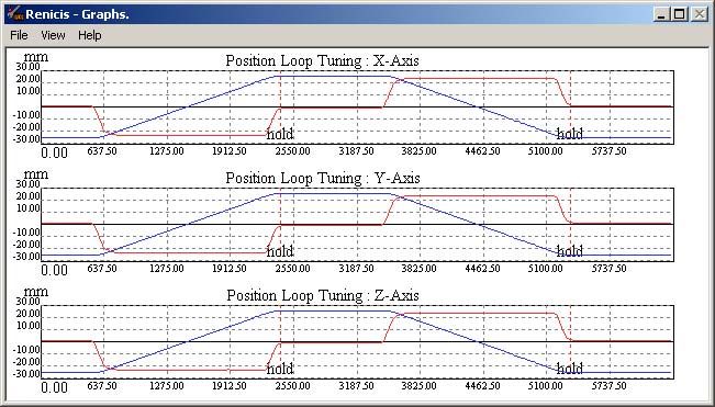
2. Follow the instructions given until the test dialog is displayed, refer to figure 19. Ensure that the default
value of 0.2 is indicated, then click on the "Start" button. The machine should move in a forward and
reverse cycle in all three axes. The following error present during the move is displayed in graphical
format. Examine the graphs produced (refer to figure 20).
Figure 19
3. If the machine runs smoothly and no periodic oscillations are apparent (refer to figure 20). The
uncompensated gain can be increased (either directly in the edit box, or by clicking on the upper 'spin'
button to the right of the edit box) by approximately 10%, now referred to as KP1, and the test repeated
by clicking on the "Start" button again.
Continue increasing the value of KP1 until one of the axes reaches the brink of instability (refer to
figure 21), then reduce the value by approximately 20% to give a stability margin and re-check for
stability. If the system is stable and no oscillations are apparent then this value is called the
“Uncompensated Proportional Gain” KP2 (and is set automatically to be the same for all axes).
NOTE: On some systems, and with very low gains, it is possible that timeouts will occur during the move.
Should this occur, increase the position tolerance by changing the value in the edit box provided. The new
value will take effect at the beginning of the next move, i.e. it will not make any effect whilst the system is
moving.24 Digital SPA commissioning sequence
Figure 20
Figure 21
If any axes become unstable (Y axis in figure 21), reduce KP1 by 20% and check again, see step 2.
NOTE: All axes must have the same KP1. The value of KP2 must be such that ALL axes display stability.Digital SPA commissioning sequence 25
2.3.2 Applying acceleration feedback
Acceleration feedback is another level of control that selectively increases the apparent inertia of the
machine, allowing the gain to be increased still further before the machine becomes unstable. Machines
react in different ways to acceleration feedback so the amount of gain increase can vary between zero and
ten times.
NOTE: Experience has shown that the use of acceleration feedback is usually not required and therefore
not recommended for machines that have an uncompensated gain of ≥ 0.2.
1. The first stage is to increase the proportional uncompensated gain value so that the machine is just
unstable using the uncompensated gain step, refer to 2.3.1, record which axes are unstable.
2. It is now necessary to activate the acceleration feedback term (KA ) in the axes that are unstable.
• Enter the machine configuration screen
• Select the "ServoConfiguration" tab and scroll down to locate the edit boxes for the
acceleration feedback terms KA(X), KA(Y) and KA(Z).
• Set the initial acceleration feedback value (KA) for the axis that has shown signs of instability
to 0.00005. Repeat for each unstable axis (Note: For any stable axes the acceleration
feedback value remains set to zero).
• Check for stability by running the “Uncompensated Gain Test refer to 2.3.1
3. If the machine is stable, increase the uncompensated gain by a further 10 – 20%. If the machine is
displaying instability as for the Y axis in figure 21, increase the value of KA (refer to step 2) in the
unstable axes by a further 0.00005 (to do this follow step 2) and repeat the uncompensated gain
test.
• If the acceleration feedback value is too high the machine will produce an audible singing
noise and must be reduced by 10 to 20 % in the unstable axes. Run the “Uncompensated
Gain Test refer to 2.3.1 to ensure the machine is stable. If it is not stable repeat this step.
4. Repeat these steps, raising the values of KA and KP1 until final values of KA and KP are found (see
figure 22). The final value of KP obtained during this process is referred to as KP3.
This will be the new “Uncompensated Gain”.
NOTE: It is necessary to increase the amount of acceleration feedback slowly in iterative steps as shown
in figure 22, so that the maximum value of KP can be found. This is in the peak between gain induced
instability line and acceleration induced instability line. The consequence of increasing the acceleration
feedback in one large step without increasing the proportional gain on intermediate steps is illustrated in
figure 23, note the final value of KP is far lower than in that obtained in figure 22.
Once the values for acceleration feedback are determined they must be left unchanged. Their values may
be different, but the value of KP3 must be the same for each axis.26 Digital SPA commissioning sequence
Figure 22
Figure 23
NOTE: At this point, if the positioning is good enough (within specifications), then no further tuning will be
necessary.Digital SPA commissioning sequence 27
2.4 Servo tuning
2.4.1 Servo tuning test
The servo tuning test is used to check the steady state error for the installation
Ensure button is not depressed and operate the button on the RENICIS toolbar. Highlight the
“Servo Tuning” step on the list of steps, run the “Servo Tuning” test by clicking the “Go to Step” button.
The dialog box shown in figure 24 will appear:
Figure 24
If a position tolerance, other than the default 100 microns, was required to prevent timeouts during moves
with the uncompensated gain value, enter the same tolerance in edit box provided here. If you know what
your desired steady-state error is then also enter that value.28 Digital SPA commissioning sequence
Start the test by clicking on the ‘Start’ button. The test may be aborted at any time after starting. The
following dialog picture (figure 25) shows the first move in progress:
Figure 25
At the beginning of this test, four different moves are performed and a worst-case steady-state error value
determined and displayed. You may wish to wait until this value is displayed before entering your desired
value, in which case, ensure that the 'Pause …' check-box has been checked before clicking on the 'Start'
button.
If the desired steady state error is achieved at the end of this test then the following screen will appear
(see figure 26). This states that performance will be degraded if the test is continued and filter parameters
calculated.
Figure 26
If the desired steady state error is not achieved, the system bandwidth is determined by performing a
series of sinusoidal moves in each axis to calculate the system gain. The above screen-shot (figure 25)
shows that the system bandwidth has not yet been determined.
Once the bandwidth has been determined, the new values for proportional gain and filters are calculated,
saved and sent to the controller. The system then performs a full 'Performance Test'. Once this is
complete, the 'View Report' button will be enabled, allowing the results of the Performance test to be
reviewed. With 'All Results' unchecked, only the worst-case results will be displayed in the report. With 'All
Results' checked, all results will be displayed in the report. From the report viewer, the report may be
saved for future viewing.
At the end of this test the option is given to enter the Manual Servo Tuning screen where it is possible to
check the machine performance. The Manual Servo Tuning step can also be accessed from the Utilities
menu.Digital SPA commissioning sequence 29
2.4.2 Servo tuning adjustment
At this stage, when the main tuning process has been completed, small adjustments can be made to
optimise the performance for a particular machine. In most cases this will not be necessary and you can
proceed to the following section.
The servo tuning objective is to find the controller parameters that meet the performance requirements for
a specific application.
Typical requirements are :
• Stability
• High disturbance rejection (reflected through a high proportional gain)
• Steady state error required (precision achievable)
• Very little or no overshoot
• Small rise time and small settling time i.e. quick response.
• Small tunnelling error (specified by user) for trajectory following applications.
The following table shows the effect of a change in the controller parameters. It is a guidance table for the
effect of change in proportional gain, lead or lag terms in the system.
The lead and lag terms Ta1 and Ta2 will only be present if the second half of the servo tuning test was
performed i.e. the desires steady state error was not achieved using simple gains so a lead / lag filter was
applied.
Speed of Precision
Overshoot Stability
response steady state
(Higher) (Higher) (Lower) (Higher)
KP (Higher)
Better Worse Worse Better
(Lower) (Lower) (Higher) (Lower)
KP (Lower)
Worse Better Better Worse
(Lower) (Higher) (Higher)
Ta2 (Higher) No Effect
Worse Worse Better
(Higher) (Lower) (Lower)
Ta2 (Lower) No Effect
Better Better Worse
(Higher) (Lower) (Lower)
Ta1 (Higher) No Effect
Better Better Worse
(Lower) (Higher) (Higher)
Ta1 (Lower) No Effect
Worse Worse Better
KP is the proportional gain of the controller.
Ta1 is the time constant corresponding to the zero.
A higher value for Ta1 means higher lead.
Ta2 is the time constant corresponding to the pole.
A higher value for Ta2 means higher lag.30 Digital SPA commissioning sequence
As the table shows, the parameters are inter-dependent making the tuning process far from trivial.
You must be using the manual servo tuning utility if you want to adjust any of these parameters and the
test performed if any parameters are changed. This will demonstrate the effectiveness of the change.
If the amount of overshoot is a concern this can be reduced along with the following error by applying
velocity feed-forward, as details in the following section.
2.4.3 Applying velocity feed-forward
Velocity feed-forward is a tuning parameter that is used to reduce the system following error. It may be
needed if the following error is unacceptably high or if the use of filters and dynamic integrator have
induced overshoot for short moves with high acceleration. Overshoot is caused by either a lack of
stiffness in the servo system or if the servo system is too responsive (tight), so this parameter is used to
get the optimum balance between the two.
1. Activate the manual servo tuning test.
2. Select tests 3 and 4 as shown in figure 27 below:
Figure 27
3. Click the Start button to run the selected tests initially with no value in the Vff input box. When the
test has completed note the values of peak following error and overshoot for all axes. The results
shown in figure 27 show a low value for the overshoot but a high following error.
4. Now add Vff, 0.01 is a good starting value and run the test again.Digital SPA commissioning sequence 31
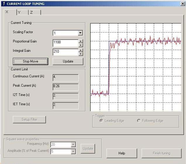
Figure 28
You can see the results shown in figure 28 give a much reduced following error and very little
change in overshoot.
5. Increasing Vff further will reduce following error, however if too much is applied overshoot will
increase to excessive levels and the machine may become unstable whilst performing the point to
point moves. Some experimentation in the Vff value will be required. Figure 29 below shows the
effect of applying too much Vff. Although the following error has reduced to a low value the amount
of overshoot has increased significantly.
Figure 29
2.4.4 Scanning tuning procedure
The tuning procedure up to this point has concentrated on getting a well tuned responsive machine that
will work well for touch-trigger applications. If it is required to scan on the CMM further tuning optimisation
will be required. Tuning for scanning is now incorporated in the UCCassist utility and is documented in
the UCCassist user’s guide (Renishaw part number H-1000-5224).32 Digital SPA commissioning sequence
2.5 Torque mode tuning procedure
Torque mode is used where motors with no tachometer or encoder feedback are fitted. In this case, the
machine velocity is derived from the scales.
2.5.1 Initial steps
In the Torque Mode section of the .ini file
Set Control mode = 1
Set the Feedback gain X,Y and Z to (10 / Maximum Move Speed). For example if the machine maximum
move speed was 250 mm/s, the Feedback gain would be set to 0.04.
Figure 30
Keep all other values as default. Press Save and then Exit.
Follow the installation steps as detailed in section 2.2.1.
2.5.2 SPA2 configuration screen
NOTE: In the SPA2 / SPAlite configuration step under motor feedback type it will now say ‘Torque Mode
enabled!’Digital SPA commissioning sequence 33
Figure 31
Refer to sections 2.2.2 to 2.2.5.
2.5.3 Velocity Loop tuning
This is a new step for torque mode.
Select the X axis only by unchecking the Y and Z axis boxes:
Figure 3234 Digital SPA commissioning sequence
Run the test by pressing the ‘Go’ button. You may get a plot something like the following:
Figure 33
Pressing ‘Edit X’ under Torque-mode parameters shows the following dialogue box:
Figure 34
Now increase the Velocity Proportional gain (try doubling it from 1 to 2 to start with). Press ‘Close’ and
press the ‘Go’ button to run the test again.
Increasing Velocity Proportional Gain should move the waveform closer to the demanded velocity. If
stable increase Velocity Proportional gain further.
NOTE: You will need to stop the test if operating in continuous mode before editing the parameters (they
cannot be edited and take effect whilst the machine is moving).
If the Velocity Proportional gain is set too high, instability will be seen.Digital SPA commissioning sequence 35
Figure 35
If this is the case reduce the Velocity Proportional gain until stability is achieved.
Figure 36
Next gradually increase the Velocity Integral Gain which should bring the waveform up to the demanded
value.
Some experimentation will be required here, as it will depend on machine characteristics. The value can
be between 1 and 1000 so increase in gradual steps.
Figure 37
Repeat above steps for the Y and Z axes. When satisfied with the responses press the ‘Save parameters’
box and then ‘Close’36 Digital SPA commissioning sequence
2.5.4 Position loop tuning
Select the X axis only by unchecking the Y and Z axis boxes
Figure 38
Select ‘Show Position Demand’.
Run the test by pressing the ‘Go’ button. You may get a plot something like the following:
Figure 39
Pressing ‘Edit X’ under Filter Parameters shows the following dialogue box
Figure 40Digital SPA commissioning sequence 37
Increase Gain to sharpen up the response without introducing instability:
Figure 41
Repeat for the Y and Z axis, experience has shown that the gains for each axis should be about the same
value.
Run the test again moving in all 3 axis.
Figure 42
The response for each axis should be similar. If they are not adjust the axis gains for individual axes
accordingly.38 Digital SPA commissioning sequence
As a final check select ‘Show Following Error Graph’ and run in all 3 axes.
Figure 43
Although the scale of this graph is not meaningful, the amplitude of the red line (following error) should be
about the same for each axis. If they are not, again adjust the gains accordingly so the following errors
are matched.Rotary table tuning procedure 39
3 Rotary table tuning procedure
3.1 Overview
To activate the tuning procedure within Renicis for the rotary table, it is necessary to have a fourth axis
daughtercard installed and configured in the SPA2. The machine’s configuration file must also indicate
that a rotary table is installed in the system.
When the rotary table is installed and configured, options within the motor configuration, current loop and
velocity loop tuning screens will be included.
An additional step will be included in the Renicis step list, this is the position loop tuning screen for the
rotary table. As shown in figure 30.
Figure 44
3.1.1 Initial settings
The initial values recommended for the rotary table tuning that have been obtained from experience are
listed below:
Target velocity (deg/sec) 25
Acceleration (deg/sec/sec) 75
Distance (degrees) 50
Step delay (ms) 1000
NOTE: When tuning the X, Y, and Z axes it is important that the tuning parameters are the same for each
axis, this is not the case for the ‘W’ rotary axis.40 Rotary table tuning procedure
3.2 Tuning
3.2.1 Velocity loop tuning
Select the W check box, this will only be active (enabled) when a rotary table is both detected and
enabled.
NOTE: It is not possible to perform a move in all four axes simultaneously. Selecting the 'W' axis will
automatically disable the other axes.
Initially run test using the default values by clicking the Go button.
Figure 45Rotary table tuning procedure 41
Figure 46
You may notice that the machine response amplitude does not match the demand.
If this is the case, adjust the tacho velocity feedback gain until the plots are matched. If you use the
up/down arrows the new values are applied immediately. If a value is typed in directly this will appear in
red and the update button will need to be clicked to download it to the controller.
NOTE: Decreasing the value in this box will have the effect of increasing the amplitude of the rotary table
speed.
As with setting up the axis velocity loop steps with SPA2, adjust scaling factor, proportional, integral and
derivative gain to achieve optimum performance.
3.2.2 Position loop tuning
Initially run with the default values.
Figure 4742 Rotary table tuning procedure
By clicking the ‘Edit’ button you can change the proportional gain. The default value of 1 for W proportional
gain should be suitable in most cases. A graph of position demand similar to the one shown should be
seen. It is unlikely that this value of proportional gain will need change unless instability is experienced.
Figure 48
In most cases the rotary table is used to rotate the inspection part to another angle and measurement
does not occur while it is moving. In these cases the lag between demand and position is not important.
If the rotary table is used as part of a multi-axis scan routine with measurement being taken during rotary
table motion then the following error will need to be minimised.Definitions 43 4 Definitions 4.1 Uncompensated gain The maximum stable gain (with a safety margin) that can be used to compensate the position error without the use of the lead and lag filters. 4.2 Acceleration feedback A high proportional gain is desirable for a high disturbance rejection and better precision (smaller steady state error). To allow a higher proportional gain, feedback from the acceleration acts as an electronic inertia which pushes the upper limit for the proportional gain. Furthermore, this does not interfere with any other control that may be added later (filters, etc). Thus you will be able to start at the point where you first have to tune the gain, only this time your upper limit is higher. 4.3 Dynamic integrator To be able to increase the proportional gain, an acceleration dependent, rate-varying lag that prevents windup is used. One might expect that a higher gain and lag term would induce a high overshoot, but the dynamic integrator peels off the effect of integration (lag) as the target is approached. When the target is hit, the effect of integration (which would have induced the overshoot) is eliminated. Once stationary again, the effect of the integrator is re-applied. Consequently, it is possible to have very high gains leading to a high precision and high disturbance rejection. To summarise, the integration is applied when needed and cancelled (gradually) when it is not needed (and becomes undesirable). 4.4 Velocity feed-forward Velocity feed-forward helps reduce the following error and increase the responsiveness of the system, consequently reducing overshoot due to delay. It is particularly useful for short moves used with a relatively high acceleration. This can be seen as a gain on the error that is proportional to the velocity profile which is high at constant speed and gradually increases during acceleration and decreases during deceleration. Too much gain on velocity feed-forward will result in a higher overshoot for the system’s response.
44            Definitions

4.5       I2t Time
The amount of time for which peak motor current is allowed to flow. If this is exceeded a fault indication is
software generated to protect against motor over heating. Continuous current, or anything less, will be
allowed to flow for unlimited time without fault.

4.6       IET Time
This is the current error time limit and will occur if there is a break in the loop after the DSP (e.g. no motor
power or motor not connected) or if the current servo is badly tuned. This is a software generated fault that
protects against excessive servo error in the current loop.

4.7       Overshoot (per axis)
The overshoot will be computed in absolute terms i.e.

Overshoot = max value of read position – Steady State Position.

4.8       Following error (per axis, already existing)
Following Error (t) = Read position (t) – Demand position (t)

Typical Following Error = Following Error (mid_time) averaged over 10 readings.

4.9       Steady state error (per axis)
Steady State Error = absolute value (mean of last 10 points of read position – Target position).

NOTE: This includes the RMS noise.

4.10 Settling time (per axis)
The settling time is the time difference between the theoretical time to get to HOLD and the time measured
to get to HOLD.
Definitions           45

4.11        Tunnelling error (for the 3D move)
The tunnelling error is the maximum distance between the two curves (real and demand) and is the
distance between the point read (measured) and its projection on the demand vector.

NOTE: The distance between two points in space is the modulus of the vector formed by these two points
(direction is not relevant here).
46                      Appendix

5         Appendices

5.1               Current and velocity loop filters

     UCC                                                                                    Current
    velocity                                                                                                      ADC      K1
                                                                                             Filter
    demand

                                                                                    -

                                                                                             PI                    PWM     I Sense

                                                                                        +                                              Tacho
                                                                                                                                         or
                                                                                                                                      Encoder

                                                                                                                    -1          PWM
                                                                                +
               Acceleration      Acceleration       Aff
               from velocity         filter
                                                                                    +

     +
                                          +           Forward       Forward
                            PI                         Filter 1      Filter 2
     -                                          +

                                   Derative
                        D           Filter

                                                                                                 Tacho Velocity
                                                                                                 Feedback gain
                                                                  Tacho
                                                                   Filter
                                                                                                Encoder Velocity
                                                                                                                         DAC
                                                                                                 Feedback gain

The SPA2 and SPAlite offer six different conditioning filters within the servo control loop. During the
Renicis commissioning sequence access to these filters are given at the appropriate step in the process.

Renicis can calculate either a low pass or a butterworth filter and apply it to the appropriate location.

With the exception of the tacho filter, which is set up in section 2.2.7, these filters are rarely needed and
their application is not covered in this tuning guide. Please contact Renishaw if further inormation is
required.

5.1.1             Current filter

The current loop filter can permit the reduction of noise on the servo power amplifiers current loop.

The recommended range for this filter is between 800 Hz and 2 KHz

5.1.2             Acceleration filter

The acceleration filter is only applied to the servo control system if acceleration feedforward is used, this
can reduce the noise generated by the acceleration feedforward calculation.

The recommended range for this filter is between 250 Hz and 750 Hz.
You can also read