META-AGGREGATING NETWORKS FOR CLASS-INCREMENTAL LEARNING
←
→
Page content transcription
If your browser does not render page correctly, please read the page content below
Under review as a conference paper at ICLR 2021

M ETA -AGGREGATING N ETWORKS
FOR C LASS -I NCREMENTAL L EARNING

 Anonymous authors
 Paper under double-blind review

                                            A BSTRACT

         Class-Incremental Learning (CIL) aims to learn a classification model with the
         number of classes increasing phase-by-phase. The inherent problem in CIL is
         the stability-plasticity dilemma between the learning of old and new classes, i.e.,
         high-plasticity models easily forget old classes but high-stability models are weak
         to learn new classes. We alleviate this issue by proposing a novel network ar-
         chitecture called Meta-Aggregating Networks (MANets) in which we explicitly
         build two residual blocks at each residual level (taking ResNet as the baseline ar-
         chitecture): a stable block and a plastic block. We aggregate the output feature
         maps from these two blocks and then feed the results to the next-level blocks. We
         meta-learn the aggregating weights in order to dynamically optimize and balance
         between two types of blocks, i.e., between stability and plasticity. We conduct
         extensive experiments on three CIL benchmarks: CIFAR-100, ImageNet-Subset,
         and ImageNet, and show that many existing CIL methods can be straightforwardly
         incorporated on the architecture of MANets to boost their performance.

1   I NTRODUCTION
AI systems are expected to work in an incremental manner when the amount of knowledge increases
over time. They should be capable to learn new concepts while maintaining the ability to recognize
previous ones. However, deep-neural-network-based systems often suffer from serious forgetting
problems (usually called “catastrophic forgetting”) when continuously updated using new coming
data. This is due to two facts: (i) the updates can override the knowledge acquired from the previous
data (McCloskey & Cohen, 1989; McRae & Hetherington, 1993; Ratcliff, 1990; Shin et al., 2017;
Kemker et al., 2018); and (ii) the model can not replay the entire previous data to regain the old
knowledge. To encourage the study to addressing the forgetting problems, Rebuffi et al. (2017)
defined a class-incremental learning (CIL) protocol that requires the model to do image classification
for which the training data of different classes come in a sequence of phases. In each phase, the
classifier is re-trained on new class data, and then evaluated on the test data of both old and new
classes. To prevent trivial algorithms such as storing all old data for replaying, there is a strict
memory budget — only a tiny set of exemplars of old classes can be saved in the memory.
This memory constraint causes the serious data amount imbalance between old and new classes, and
indirectly causes the main problem of CIL – stability-plasticity dilemma (Mermillod et al., 2013).
Higher plasticity results in the forgetting of old classes (McCloskey & Cohen, 1989), while higher
stability weakens the model from learning the data of new classes (containing a larger number of
samples). Existing methods try to balance stability and plasticity using simple data strategies. As
illustrated in Figure 1, they directly train the model on the imbalanced dataset (Rebuffi et al., 2017;
Li & Hoiem, 2018), and some other works include a fine-tuning step using a balanced subset of
exemplars (Castro et al., 2018; Hou et al., 2019; Douillard et al., 2020). However, these methods
turn out to be not particularly effective. For example, LUCIR (Hou et al., 2019) sees an accuracy
drop of around 16% in predicting 50 previous classes in the last phase (compared to the upper-bound
accuracy when all old samples are available) on the CIFAR-100 dataset (Krizhevsky et al., 2009).
In this paper, we address the stability-plasticity dilemma by introducing a novel network architecture
called Meta-Aggregating Networks (MANets) for CIL. Taking the ResNet (He et al., 2016b) as
an example of baseline architectures, in MANets, we explicitly build two residual blocks (at each
residual level): one for maintaining the knowledge of old classes (i.e., the stability) and the other

                                                  1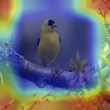
Under review as a conference paper at ICLR 2021

       old exemplars        old exemplars                                            old exemplars
                                                       old exemplars                                            old exemplars

          new data             new data                                                new data
                                            herding*   new exemplars                                 herding*   new exemplars

                                                                                     train                meta-train
        train                train                 fine-tune
                                                                                                                 aggregating
                                                                                    plastic blocks                weights 1
       new model            new model                  new model

                                                                       initialize
                                                                                                                 aggregating
                                                                                    stable blocks                 weights 2
    initialize           initialize
                                                                                                                  new model
       old model            old model                                               old model

    (a) Conventional          (b) Balanced Fine-tuning                                    (c) Meta Aggregating

Figure 1: Conceptual illustrations of different CIL methods. (a) Conventional methods use all avail-
able data (imbalanced classes) to train the model (Rebuffi et al., 2017; Hou et al., 2019) (b) Castro
et al. (2018), Hou et al. (2019) and Douillard et al. (2020) follow the convention but add a fine-tuning
step using the balanced set of exemplars. (c) Our MANets approach uses all available data to update
the plastic and stable blocks, and use the balanced set of exemplars to meta-learn the aggregating
weights. We continuously update these weights such as to dynamically balance between plastic and
stable blocks, i.e., between plasticity and stability. *: herding is the method to choose exemplars
(Welling, 2009), and can be replaced by other methods, e.g., Mnemonics Training (Liu et al., 2020).

for learning new classes (i.e., the plasticity), as shown in Figure 1(c). We achieve these by allowing
different numbers of learnable parameters in these two blocks, i.e., less learnable parameters in the
stable but more in the plastic. We apply aggregating weights to the output feature maps from these
two blocks, sum them up, and pass the results to the next residual level. In this way, we are able to
dynamically balance between the stable and plastic features, i.e., stability and plasticity, by updating
the aggregating weights. To achieve auto updating, we take these weights as hyperparmeters and
use meta-learning (Finn et al., 2017; Wu et al., 2019; Liu et al., 2020) to optimize them.
Technically, the optimization of MANets includes two steps at each CIL phase: (1) learn the net-
work parameters for two types of residual blocks, and (2) meta-learn their aggregating weights.
Step 1 is the standard training for which we use all the data available at the phase. Step 2 aims to
balance between two types of blocks for which we downsample the new class data to build a bal-
anced subset as the meta-training data, as illustrated in Figure 1(c). We formulate these two steps
in a bilevel optimization program (BOP) and conduct the optimizations alternatively, i.e., update
network parameters with aggregating weights fixed, and then switch (Sinha et al., 2018; MacKay
et al., 2019; Liu et al., 2020). For evaluation, we conduct extensive CIL experiments on three bench-
marks, CIFAR100, ImageNet-Subset, and ImageNet. We find that many existing CIL methods, e.g.,
iCaRL (Rebuffi et al., 2017), LUCIR (Hou et al., 2019), Mnemonics Training (Liu et al., 2020),
and PODNet (Douillard et al., 2020), can be straightforwardly incorporated on the architecture of
MANets, yielding consistent performance improvements.
Our contributions are thus three-fold: (1) a novel and generic network architecture consisting of
stable and plastic blocks, specially designed for tackling the problems of CIL; (2) a BOP-based
formulation and the corresponding end-to-end optimization solution that enables dynamic and auto
balancing between stable and plastic blocks; and (3) extensive experiments by incorporating the
proposed architecture into different baseline methods of CIL.

2    R ELATED W ORK

Incremental learning studies the problem of learning a model from the data that come gradually
in sequential training phases. It is also referred to as continual learning (De Lange et al., 2019a;
Lopez-Paz & Ranzato, 2017) or lifelong learning (Chen & Liu, 2018; Aljundi et al., 2017). Re-
cent approaches are either in task-incremental setting (classes from different datasets) (Li & Hoiem,
2018; Shin et al., 2017; Hu et al., 2019; Chaudhry et al., 2019; Riemer et al., 2019), or in class-

                                                           2
Under review as a conference paper at ICLR 2021

incremental setting (classes from the identical dataset) (Rebuffi et al., 2017; Hou et al., 2019; Wu
et al., 2019; Castro et al., 2018; Liu et al., 2020). Our work is conducted on the setting of the latter
one we call class-incremental learning (CIL). Incremental learning approaches can be categorized
according to the methods of tackling the problem of model forgetting. There are regularization-
based, replay-based, or parameter-isolation-based methods (De Lange et al., 2019b; Prabhu et al.,
2020). Regularization-based methods introduce regularization terms in the loss function to con-
solidating previous knowledge when learning new data. Li & Hoiem (2018) first applied the regu-
larization term of knowledge distillation (Hinton et al., 2015) in CIL. Hou et al. (2019) introduced
a series of components such as less-forgetting constraint and inter-class separation to mitigate the
negative effects caused by data imbalance (between old and new classes). Douillard et al. (2020)
proposed an efficient spatial- based distillation-loss applied throughout the model and a representa-
tion comprising multiple proxy vectors for each class. Replay-based methods store a tiny subset of
old data, and replay the model on them together with the new class data. Rebuffi et al. (2017) picked
the nearest neighbors of the average sample per class for the subset. Liu et al. (2020) parameterized
the samples in the subset and meta-optimized them in an end-to-end manner. Parameter-isolation-
based methods are mainly applied to task-incremental learning (not CIL). Related methods dedicate
different model parameters for different incremental phases, to prevent model forgetting (caused by
parameter overwritten). Abati et al. (2020) equipped each convolution layer with task-specific gating
modules which select specific filters to learn current input. Rajasegaran et al. (2019) progressively
chose the optimal paths for the new tasks meanwhile encouraging parameter sharing across tasks.
Our work is the first one proposing new network architecture for CIL. We isolate the knowledge of
old classes and the learning of new classes specially in two types of residual blocks, and meta-learn
their weights to balance between them automatically.
Meta-learning can be used to optimize hyperparameters of deep models, e.g., the aggregating
weights in our MANets. Technically, the optimization process can be formulated as a bilevel opti-
mization program where model parameters are updated at the base level and hyperparameters at the
meta level (Von Stackelberg & Von, 1952; Wang et al., 2018; Goodfellow et al., 2014). Recently,
there emerge a few of meta-learning based incremental learning methods. Wu et al. (2019) meta-
learned a bias correction layer for incremental learning models. Liu et al. (2020) parameterized data
exemplars and optimized them by meta gradient descent. Rajasegaran et al. (2020) incrementally
learned new tasks while meta-learning a generic model to retain the knowledge of all training tasks.

3     M ETA -AGGREGATING N ETWORKS (MANets)
Class incremental learning (CIL) usually assumes there are (N + 1) learning phases in total, i.e, one
initial phase and N incremental phases during which the number of classes gradually increases (Hou
et al., 2019; Liu et al., 2020; Douillard et al., 2020). In the initial phase, only data D0 is available
to train the first model Θ0 . There is a strict memory budget in CIL systems, so after the phase,
only a small subset of D0 (exemplars denoted as E0 ) can be stored in the memory to used as replay
samples in later phases. In the i-th (i ≥ 1) phase, we load the exemplars of old classes E0:i−1 =
{E0 , . . . , Ei−1 } to train model Θi together with new class data Di . Then, we evaluate the trained
model on the test data containing both old and new classes. We repeat such training and evaluation
through all phases.
The major challenge of CIL is that the model trained at new phases easily “forgets” old classes. To
tackle this, we introduce a novel architecture called MANets. MANets is based on ResNet and each
of its residual levels is composed of two different blocks: a plastic one to adapt to the new class data
and a stable one to maintain the knowledge learned from old classes. The details of this architecture
are provided in Section 3.1. The optimization steps of MANets are elaborated in Section 3.2.

3.1   T HE ARCHITECTURE OF MANets

In Figure 2(a), we provide an illustrative example of our MANets with three residual levels. The
inputs x[0] are the images and the outputs x[3] are the features for training classifiers. Every residual
level in-between consists of two parallel residual blocks: one (orange) will be actively adapted to
new coming classes while the other one (blue) has its parameters partially fixed to maintain the
knowledge learned from old classes. After feeding images to Level 1, we obtain two sets of feature
maps respectively from two blocks, and aggregate them by weight parameters α[1] . Then, we feed

                                                   3
Under review as a conference paper at ICLR 2021

          Level 1                                Level 2                               Level 3

                                     (a) Meta-Aggregating Networks (MANets)
          Level 1                                Level 2                               Level 3

                                     (b) MANets with highway connection blocks

Figure 2: (a) The architecture of MANets. For each residual level, we derive the feature maps from
stable blocks (φ θbase , blue) and plastic blocks (η, orange), respectively, aggregate them with
meta-learned weights, and feed the result in the next level. (b) An improved version of MANets by
including a highway connection block (h, green) at each level.

the resulted maps to Level 2 and repeat the steps above. The same applies to Level 3. Finally, we pool
the resulted maps after Level 3 to learn classifiers. In addition, Figure 2(b) provides an improved
version of MANets by including a highway connection block (green) at each residual level. Below
we discuss (i) the design and benefits of the dual-branch residual blocks; (ii) the operations for
feature extraction and aggregation; and (iii) the design and benefits of highway connection blocks.
Stable and plastic blocks at each residual level. We aim to balance between the plasticity (for
learning new classes) and stability (for maintaining the knowledge of old classes) using a pair of
stable and plastic blocks at each residual level. We achieve this by allowing different numbers
of learnable parameters in two blocks, i.e., less learnable parameters in the stable but more in the
plastic. We detail the operations in the following. We denote the learnable parameters as η and φ
for the plastic and stable blocks respectively (at any CIL phase). η contains all the convolutional
weights, while φ contains only the neuron-level scaling weights (Sun et al., 2019) which are applied
on the frozen convolutional neural network θbase pre-learned at the 0-th phase1 . As a result, the
number of learnable parameters φ is much less than that of η. For example, when using the neurons
                                                                                   1
of size 3 × 3 in θbase , the number of learnable parameters φ is reduced to only 3×3  of the original
number (i.e. the number of learnable parameters in η). More details are provided in the appendices.
                                                         [k]
Feature extraction and aggregation. Let Fµ (·) denote the transformation function corresponding
to the residual block with parameters µ at Level k. Given a batch of training images x[0] , we feed
them to MANets and compute the feature maps at the k-th level (through the stable and plastic
blocks respectively) as follows,
                               [k]      [k]              [k−1]
                             xφ = Fφ          θbase (x           );   x[k]  [k] [k−1]
                                                                       η = Fη (x      ).                       (1)
The transferabilities (of the knowledge learned from old classes) are different at different levels
of neural networks (Yosinski et al., 2014). Therefore, it is important to apply different aggregating
                                   [k]    [k]
weights for different levels. Let αφ and αη denote the aggregating weights of the stable and plastic
                                                                                                      [k]       [k]
blocks respectively at the k-th level, based on which we compute the weighted sum of xφ and xη
as follows,
                                             [k]  [k]
                                    x[k] = αφ · xφ + αη[k] · xη[k] .                         (2)
In our illustrative example in Figure 2(a), there are three pairs of weights at each phase. Hence, it
becomes increasingly challenging to determine all the weights/hyperparamters if multiple phases are
    1
      Related works (Hou et al., 2019; Douillard et al., 2020; Liu et al., 2020) learned Θ0 in the 0-th phase using
half of the total classes. We follow the same way to train Θ0 and then freeze it as θbase .

                                                                 4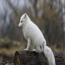
Under review as a conference paper at ICLR 2021

involved. In this paper, we propose a meta-learning strategy to automatically adapt these weights,
i.e., meta-optimizing the weights for different blocks at each phase, see details in Section 3.2.
Highway connection blocks. Highway network aims to address the vanishing gradients problem in
deep neural networks (Srivastava et al., 2015). From the view of the network architecture, adding
highway connection modifies our dual-block architecture to be a residual one where the highway
plays the role of an identity branch (except that it has a gating mechanism) (He et al., 2016a). In
specific, at each residual level, we add a block of 1 × 1 convolution layers (stride=2) and denote it
as h. We thus can rewrite Eq. 2 as follows,
                           [k]    [k]                           [k]             [k]       [k]
                x[k] = αφ · xφ + αη[k] · xη[k] + xh ,                 where    xh = Fh (x[k−1] ).             (3)

When there are K levels in MANets (with or without highway at each level), we use the feature
maps after the highest level x[K] to train classifiers.

3.2   B ILEVEL OPTIMIZATION PROGRAM FOR MANets

In each incremental phase, we optimize two groups of learnable parameters in MANets: (a) the scal-
ing weights φ on stable blocks, the convolutional weights η on plastic blocks, and the convolutional
weights h on highway blocks; (b) the aggregating weights α. The former is for network parameters
and the latter is for hyperparameters. Therefore, we formulate the overall optimization process as a
bilevel optimization program (BOP) (Goodfellow et al., 2014; Liu et al., 2020).
BOP formulation. In our MANets, the network parameters [φ, η, h] are trained using the aggre-
gating weights α as hyperparameters. In turn, α can be updated based on the learned network
parameters [φ, η, h]. In this way, the optimality of [φ, η, h] imposes a constraint on α and vise versa.
Ideally, in the i-th phase, the CIL system aims to learn the optimal αi and [φi , ηi , hi ] that minimize
the classification loss on all training samples seen so far, i.e., Di ∪ D0:i−1 , so the (ideal) BOP can
be formulated as,
                        min L(αi , φ∗i , ηi∗ , h∗i ; D0:i−1 ∪ Di )                                           (4a)
                         αi
                        s.t. [φ∗i , ηi∗ , h∗i ] = arg min L(αi , φi , ηi , hi ; D0:i−1 ∪ Di ),               (4b)
                                                [φi ,ηi ,hi ]

where L(·) denotes the loss function, e.g., cross-entropy loss. Please note that for the conciseness of
the formulation, we use φi to represent φi θbase (same in the follows). Following Liu et al. (2020),
we call Problem 4a and Problem 4b as meta-level and base-level problems, respectively.
Data strategy. To solve Problem 4, we need to use D0:i−1 . However, in the setting of CIL (Rebuffi
et al., 2017; Hou et al., 2019; Douillard et al., 2020), we cannot access D0:i−1 but only a small set of
exemplars E0:i−1 , e.g., 20 samples of each old class. Directly replacing D0:i−1 ∪Di with E0:i−1 ∪Di
in Problem 4 will lead to the forgetting problem for the old classes. To alleviate this, we propose
a new data strategy in which we use different training data splits to learn different parameters: (i)
in the meta-level problem, αi is used to balance the stable and the plastic blocks, so we use the
balanced subset to update it, i.e., meta-training αi on E0:i−1 ∪ Ei ; (ii) in the base-level problem,
[φi , ηi , hi ] are the network parameters used for feature extraction, so we leverage all the available
data to learn them, i.e., base-training [φi , ηi , hi ] on E0:i−1 ∪ Di . In this way, we reformulate the ideal
BOP in Problem 4 as a solvable BOP provided below,
                        min L(αi , φ∗i , ηi∗ , h∗i ; E0:i−1 ∪ Ei )                                           (5a)
                          αi
                         s.t. [φ∗i , ηi∗ , h∗i ] = arg min L(αi , φi , ηi , hi ; E0:i−1 ∪ Di ).              (5b)
                                                [φi ,ηi ,hi ]

Updating parameters. We solve the BOP by updating the two groups of parameters (αi and
[φ, η, h]) alternatively across epochs, i.e., the j-th epoch for learning one group and the (j + 1)-
th epoch for the other group until both groups converge. First, we initialize αi , φi , ηi and hi with
αi−1 , φi−1 , ηi−1 and hi−1 , respectively. Please note that φ0 is initialized with ones, following Sun
et al. (2019), η0 is initialized with θbase , and α0 is initialized with 0.5. Based on our Data strategy,
we use all available data in the i-th phase to solve the base-level problem, i.e., base-learning [φi , ηi ,
hi ] as follows,
                [φi , ηi , hi ] ← [φi , ηi , hi ] − γ1 ∇[φi ,ηi ,hi ] L(αi , φi , ηi , hi ; E0:i−1 ∪ Di ).    (6)

                                                                5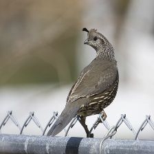
Under review as a conference paper at ICLR 2021
Then, we use a balanced exemplar set to solve meta-level problem, i.e., meta-learning αi as follws,
αi ← αi − γ2 ∇αi L(αi , φi , ηi , hi ; E0:i−1 ∪ Ei ), (7)
where γ1 and γ2 are the base-level and meta-level Algorithm 1 MANets (in the i-th phase)
learning rates, respectively. Algorithm 1 summa-
1: Input: New class data Di ; old class exemplars
rizes the training algorithm of the proposed MANets,
taking the i-th CIL phase as an example. E0:i−1 ; old parameters αi−1 , φi−1 , ηi−1 , and
hi−1 ; base model θbase .
2: Output: new parameters αi , φi , ηi , and hi ; new
4 E XPERIMENTS class exemplars Ei .
3: Get Di and load E0:i−1 from memory;
We evaluate the proposed MANets on three CIL 4: Initialize [φi , ηi , hi ] with [φi−1 , ηi−1 , hi−1 ];
benchmarks, i.e., CIFAR-100 (Krizhevsky et al., 5: Initialize αi with αi−1 ;
2009), ImageNet-Subset (Rebuffi et al., 2017) and 6: Select exemplars Ei $ Di by herding;
ImageNet (Russakovsky et al., 2015), and achieve 7: for epochs do
the state-of-the-art performance. Below we de-
8: for mini-batch in E0:i−1 ∪ Di do
scribe the datasets and implementation details (Sec-
9: Train [φi , ηi , hi ] on E0:i−1 ∪ Di by Eq. 6;
tion 4.1), followed by the results and analyses (Sec-
tion 4.2) including comparisons to related methods, 10: end for
ablation studies and visualization results. 11: for mini-batch in E0:i−1 ∪ Ei do
12: Meta-train αi on E0:i−1 ∪ Ei by Eq. 7;
13: end for
4.1 DATASETS AND IMPLEMENTATION DETAILS
14: end for
Datasets. We conduct CIL experiments on two 15: Update exemplars Ei by herding;
datasets, CIFAR-100 (Krizhevsky et al., 2009) and 16: Replace E0:i−1 with E0:i−1 ∪ Ei in the memory.
ImageNet (Russakovsky et al., 2015), following re-
lated works (Hou et al., 2019; Liu et al., 2020; Douillard et al., 2020). ImageNet is used in two CIL
settings: one based on a subset of 100 classes (ImageNet-Subeset) and the other based on the entire
1, 000 classes. The 100-class data for ImageNet-Subeset are randomly sampled from ImageNet with
an identical random seed (1993) by NumPy, following Hou et al. (2019); Liu et al. (2020).
Implementation details. Following the uniform setting (Douillard et al., 2020; Liu et al., 2020),
we use a 32-layer ResNet for CIFAR-100 and an 18-layer ResNet for ImageNet. The learning rates
γ1 and γ2 are initialized as 0.1 and 1 × 10⁻⁵ , respectively. We impose a constraint on α, i.e.,
αη + αφ = 1 for each block. For CIFAR-100 (ImageNet), we train the model for 160 (90) epochs
in each phase, and the learning rates are divided by 10 after 80 (30) and 120 (60) epochs. We use an
SGD optimizer with momentum to train the model.
Benchmark protocol. This work follows the protocol in Hou et al. (2019), Liu et al. (2020), and
Douillard et al. (2020). Given a dataset, the model is firstly trained on half of the classes. Then, it
learns the remaining classes evenly in the subsequent phases. Assume there is an initial phase and
N incremental phases for the CIL system. N is set to be 5, 10 or 25. At each phase, the model is
evaluated on the test data for all seen classes. The average accuracy (over all phases) is reported.
4.2 R ESULTS AND ANALYSES
Table 1 shows the results of 4 baselines with and without our MANets as a plug-in architecture,
and some other related works. Table 2 demonstrates the results in 8 ablative settings. Figure 3
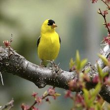
visualizes the Grad-CAM (Selvaraju et al., 2017) activation maps obtained from different residual
blocks. Figure 4 shows our phase-wise results compared to those of baselines. Figure 5 shows the
changes of values for αη and αφ across 10 incremental phases.
Comparing with the state-of-the-arts. Table 1 shows that taking our MANets as a plug-in archi-
tecture on 4 baseline methods (Rebuffi et al., 2017; Hou et al., 2019; Liu et al., 2020; Douillard et al.,
2020) consistently improves their performance. E.g., on CIFAR-100, “LUCIR + MANets” achieves
3% of improvement on average. In Figure 4, we can observe that our method achieves the highest
accuracy in all settings, compared to the state-of-the-arts. Interestingly, we find that our MANets
can boost the more performance for the simpler baseline methods, e.g., iCaRL. “iCaRL + MANets”
achieves better results than those of LUCIR on ImageNet-Subset, even though the latter method uses
a series of regularization techniques.
6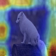
Under review as a conference paper at ICLR 2021

                                         CIFAR-100          ImageNet-Subset            ImageNet
Method
                                     N =5    10       25     5     10     25       5      10      25
LwF (Li & Hoiem, 2018)               49.59 46.98 45.51     53.62 47.64 44.32     44.35 38.90 36.87
BiC (Wu et al., 2019)                59.36 54.20 50.00     70.07 64.96 57.73     62.65 58.72 53.47
TPCIL (Tao et al., 2020)             65.34 63.58   –       76.27 74.81   –       64.89 62.88   –
iCaRL (Rebuffi et al., 2017)         57.12 52.66 48.22     65.44 59.88 52.97     51.50 46.89 43.14
 + MANets (ours)                     64.11 60.22 56.40     73.42 71.76 69.21     63.74 61.19 56.92
LUCIR (Hou et al., 2019)             63.17 60.14 57.54     70.84 68.32 61.44     64.45 61.57 56.56
 + MANets (ours)                     67.12 65.21 64.29     73.25 72.19 70.95     64.62 62.22 60.60
Mnemonics (Liu et al., 2020)         63.34 62.28 60.96     72.58 71.37 69.74     64.54 63.01 61.00
 + MANets (ours)                     67.37 65.64 63.29     73.13 72.06 70.75     64.90 63.42 61.45
PODNet-CNN (Douillard et al., 2020) 64.83 63.19 60.72      75.54 74.33 68.31     66.95 64.13 59.17
 + MANets (ours)                    66.12 64.11 62.12      76.63 75.40 71.43     67.60 64.79 60.97

Table 1: Average incremental accuracy (%) of four CIL methods with and without our MANets
as a plug-in architecture, and the related methods. Please note (1) Douillard et al. (2020) didn’t
report the results for N =25 on the ImageNet, so we produce the results using their public code;
(2) Liu et al. (2020) updated the results on arXiv version (after fixing a bug in their code), differ-
ent from its conference version; (3) Highway connection blocks are applied in our MANets; and
(4) For CIFAR-100, we use “all”+“scaling” blocks. For ImageNet-Subeset and ImageNet, we use
“scaling”+“frozen” blocks. Please refer to Section 4.2 Ablation settings for details.

Ablation settings. Table 2 demon-
strates the ablation study. Block Row Ablation Setting               CIFAR-100      ImageNet-Subset
types: by differentiating the num-                               N =5 10       25    5    10    25
bers of learnable parameters, we         1     only single “all” 63.17 60.14 57.54 70.84 68.32 61.44
have 3 block types: (1) “all”            2       “all” + “all”   64.49 61.89 58.87 69.72 66.69 63.29
means learning all the convolu-          3     “all” + “scaling” 66.21 65.17 63.45 71.38 69.11 67.40
tional weights and biases; (2)           4     “all” + “frozen”  65.62 64.05 63.67 71.71 69.87 67.92
“scaling” means learning neuron-         5 “scaling” + “frozen” 64.71 63.65 62.89 73.01 71.65 70.30
level scaling weights (Sun et al.,       6       w/ highway      67.12 65.21 64.29 71.98 70.36 69.35
2019) on the top of a frozen             7      w/o balanced E   65.91 64.70 63.08 70.30 69.92 66.89
                                         8 w/o meta-learned α 65.89 64.49 62.89 70.31 68.71 66.34
base model θbase ; and (3) “frozen”
means using θbase (frozen) as
the feature extractor of the sta- Table 2: Ablation results (%). The baseline (Row 1) is LU-
ble block. Rows 1 is the base- CIR. Meta-learned α are applied for Rows 3-7. Rows 6-8
line model of LUCIR (Hou et al., are based on “all”+“scaling”. Note that highway connection
2019). Row 2 is a double-block blocks are applied only on Row 6.
version of LUCIR. They are with-
out meta-learning. Rows 3-5 are our MANets using different pairs of blocks. Row 6-8 use
“all”+“scaling”, and under the setting of: (1) Row 6 includes highway connection blocks; (2) Row 7
uses imbalanced data E0:i−1 ∪Di to meta-train α; and (3) Row 8 simply uses fixed weights αη = 0.5
and αφ = 0.5 at each residual level.
Ablation results. Comparing the second block of results (Rows 3-5) to the first block (baseline),
it is obvious that using the proposed MANets can significantly improve the performance of incre-
mental learning, e.g. an average of over 6% gain on ImageNet-Subset (N = 25). From Rows 3-5,
we can observe that on ImageNet-Subset, the model with fewer learnable parameters (“scaling”+
“frozen”) works the best. This is because we use a shallower network for the larger dataset follow-
ing the benchmark protocol (ResNet-32 for CIFAR-100; ResNet-18 for ImageNet-Subset), so θbase
for ImageNet-Subset is well-learned in the initial phase and can offer high-quality features for later
phases. Comparing Row 6 to Row 3, it is clear that highway connection is helpful for all settings.
Comparing Row 7 to Row 3, it shows the importance of using balanced subset to meta-optimize
α. Comparing Row 8 to Row 3, it shows the superiority of meta-learned α (that is dynamic and
optimal) over manually-chosen α.

                                                  7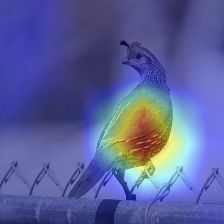
Under review as a conference paper at ICLR 2021

                                                                                                                                                          can opener Arctic fox Arctic fox
                                   goldfinch goldfinch
         Classes seen in Phase 0

                                                                                                                                Classes seen in Phase 5
  49

  37

  176
                                   quail

4840
                                                         image   MANets   stable   plastic                                                                                                   image    MANets         stable        plastic

4872    Figure 3: The activation maps using Grad-CAM (Selvaraju et al., 2017) for Phase 5 (the last phase)

                                                                                                                       Classes seen in Phase 5
                                                                                                                                                    Arctic fox
4811
        model on ImageNet-Subset (N =5). Samples are selected from the classes coming in Phase 0 (left)
        and Phase 5 (right), respectively. Green tick (red cross) means the discriminative features are acti-
        vated on the object regions successfully (unsuccessfully). ᾱη = 0.428 and ᾱφ = 0.572.

                                                                                                       can opener Arctic fox
4981

        The visualization of activation maps.                                                          UpperBound                                                                                    PODNet          LUCIR         iCaRL
        Figure 3 shows the activation maps vi-                                                         MANets (ours)                                                                                 Mnemonics       BiC           LwF
        sualized by Grad-CAM for Phase 5 (last
                                          baseline
        phase) model on ImageNet-Subset          (N =5).
                                                                                                                               image                                                           MANets       stable       plastic
        The visualized samples (on the left and
        right) are from the classes coming in Phase
        0 and Phase 5, respectively. When input
        Phase 0 samples to the Phase 5 model, it
        activates the object regions on the stable
        block but fails on the plastic block. It is
        easy to explain as the plastic block already
        forgets the knowledge learned in Phase 0                                             Figure 4: Phase-wise accuracy on CIFAR-100. “Up-
        while the stable block successfully retains                                          per Bound” shows the results of joint training with all
        it. This situation is reversed when input                                            previous data accessible in each phase. The average
        Phase 5 samples to that model. It is be-                                             accuracy of each curve is reported in Table 1, and our
                       0 block
        cause the stable    1 is2 far3less4learnable
                                                   5 6                                        7 8are 9on the
                                                                                             results       10row
                                                                                                               11of12    13 14 15
                                                                                                                     “Mnemonics        16 17 18 19
                                                                                                                                   + MANets”.                                                                                                20 21 22 23 24
        and fails to adapt to the new coming data.
        While for all samples, our MANets can                                                  2                                                                                             #phase (N=25)
        capture the right object features, as it ag-                                           1
        gregates the feature maps from two types
        of blocks and its meta-learned aggregat-                                               0
        ing weights ensure the effective adaptation
                                                                                              -1
        (balancing between two types of blocks) in                                                 0 2 4 6 8 10 0 2 4 6 8 10 0 2 4 6 8 10
        both early and late phases.                                                             #phases (Level 1) #phases (Level 2) #phases (Level 3)
        The values of αη and αφ . Figure 5 shows Figure 5: The changes of values for α and α on
                                                                                                    η       φ
        the changes of values for αη and αφ on CIFAR-100 (N =10). All curves are smoothed with a
        CIFAR-100 (N =10). We can see that rate of 0.8 for a better visualization. More results are
        Level 1 tends to get larger values of αφ , provided in the appendices.
        while Level 3 tends to get larger values of
        αη , i.e., lower-level residual block learns to be stabler which is intuitively correct in deep models.
        Actually, the CIL system is continuously transferring its learned knowledge to subsequent phases.
        Different layers (or levels) of the model have different transferabilities (Yosinski et al., 2014). Level
        1 encodes low-level features that are more stable and shareable among classes. Level 3 nears the
        classifiers, and it tends to be more plastic such as to fast to adapt to new coming data.

        5                              C ONCLUSIONS
        In this paper, we introduce a novel network architecture MANets for class-incremental learning
        (CIL). Our main contribution lies in addressing the issue of stability-plasticity dilemma by aggre-
        gating the feature maps from two types of residual blocks (i.e., stable and plastic blocks) for which
        the aggregating weights are optimized by meta-learning in an end-to-end manner. Our approach is
        generic and can be easily incorporated into existing CIL methods to boost the performance.

                                                                                                   8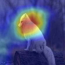
Under review as a conference paper at ICLR 2021

R EFERENCES
Davide Abati, Jakub Tomczak, Tijmen Blankevoort, Simone Calderara, Rita Cucchiara, and
  Babak Ehteshami Bejnordi. Conditional channel gated networks for task-aware continual learn-
  ing. In CVPR, pp. 3931–3940, 2020.
Rahaf Aljundi, Punarjay Chakravarty, and Tinne Tuytelaars. Expert gate: Lifelong learning with a
  network of experts. In CVPR, pp. 3366–3375, 2017.
Francisco M. Castro, Manuel J. Marı́n-Jiménez, Nicolás Guil, Cordelia Schmid, and Karteek Ala-
  hari. End-to-end incremental learning. In ECCV, pp. 241–257, 2018.
Arslan Chaudhry, Marc’Aurelio Ranzato, Marcus Rohrbach, and Mohamed Elhoseiny. Efficient
  lifelong learning with a-gem. In ICLR, 2019.
Zhiyuan Chen and Bing Liu. Lifelong machine learning. Synthesis Lectures on Artificial Intelligence
  and Machine Learning, 12(3):1–207, 2018.
Matthias De Lange, Rahaf Aljundi, Marc Masana, Sarah Parisot, Xu Jia, Aleš Leonardis, Gregory
 Slabaugh, and Tinne Tuytelaars. A continual learning survey: Defying forgetting in classification
 tasks. arXiv, 1909.08383, 2019a.
Matthias De Lange, Rahaf Aljundi, Marc Masana, Sarah Parisot, Xu Jia, Ales Leonardis, Gregory
 Slabaugh, and Tinne Tuytelaars. Continual learning: A comparative study on how to defy forget-
 ting in classification tasks. arXiv, 1909.08383, 2019b.
Arthur Douillard, Matthieu Cord, Charles Ollion, Thomas Robert, and Eduardo Valle. Podnet:
  Pooled outputs distillation for small-tasks incremental learning. In ECCV, 2020.
Chelsea Finn, Pieter Abbeel, and Sergey Levine. Model-agnostic meta-learning for fast adaptation
  of deep networks. In ICML, pp. 1126–1135, 2017.
Ian Goodfellow, Jean Pouget-Abadie, Mehdi Mirza, Bing Xu, David Warde-Farley, Sherjil Ozair,
  Aaron Courville, and Yoshua Bengio. Generative adversarial nets. In NIPS, pp. 2672–2680,
  2014.
Kaiming He, Xiangyu Zhang, Shaoqing Ren, and Jian Sun. Identity mappings in deep residual
  networks. In Bastian Leibe, Jiri Matas, Nicu Sebe, and Max Welling (eds.), ECCV, pp. 630–645.
  Springer, 2016a.
Kaiming He, Xiangyu Zhang, Shaoqing Ren, and Jian Sun. Deep residual learning for image recog-
  nition. In CVPR, pp. 770–778, 2016b.
Geoffrey E. Hinton, Oriol Vinyals, and Jeffrey Dean. Distilling the knowledge in a neural network.
  arXiv, 1503.02531, 2015.
Saihui Hou, Xinyu Pan, Chen Change Loy, Zilei Wang, and Dahua Lin. Learning a unified classifier
  incrementally via rebalancing. In CVPR, pp. 831–839, 2019.
Wenpeng Hu, Zhou Lin, Bing Liu, Chongyang Tao, Zhengwei Tao, Jinwen Ma, Dongyan Zhao,
 and Rui Yan. Overcoming catastrophic forgetting for continual learning via model adaptation. In
 ICLR, 2019.
Ronald Kemker, Marc McClure, Angelina Abitino, Tyler L. Hayes, and Christopher Kanan. Mea-
  suring catastrophic forgetting in neural networks. In AAAI, pp. 3390–3398, 2018.
Alex Krizhevsky, Geoffrey Hinton, et al. Learning multiple layers of features from tiny images.
  Technical report, Citeseer, 2009.
Zhizhong Li and Derek Hoiem. Learning without forgetting. IEEE Transactions on Pattern Analysis
  and Machine Intelligence, 40(12):2935–2947, 2018.
Yaoyao Liu, Yuting Su, An-An Liu, Bernt Schiele, and Qianru Sun. Mnemonics training: Multi-
  class incremental learning without forgetting. In CVPR, pp. 12245–12254, 2020.

                                                9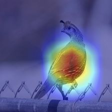
Under review as a conference paper at ICLR 2021

David Lopez-Paz and Marc’Aurelio Ranzato. Gradient episodic memory for continual learning. In
  NIPS, pp. 6467–6476, 2017.
Matthew MacKay, Paul Vicol, Jon Lorraine, David Duvenaud, and Roger Grosse. Self-tuning net-
 works: Bilevel optimization of hyperparameters using structured best-response functions. In
 ICLR, 2019.
Michael McCloskey and Neal J Cohen. Catastrophic interference in connectionist networks: The
 sequential learning problem. In Psychology of Learning and Motivation, volume 24, pp. 109–165.
 Elsevier, 1989.
K. McRae and P. Hetherington. Catastrophic interference is eliminated in pre-trained networks. In
  CogSci, 1993.
Martial Mermillod, Aurélia Bugaiska, and Patrick Bonin. The stability-plasticity dilemma: Inves-
 tigating the continuum from catastrophic forgetting to age-limited learning effects. Frontiers in
 Psychology, 4:504, 2013.
Ameya Prabhu, Philip HS Torr, and Puneet K Dokania. Gdumb: A simple approach that questions
 our progress in continual learning. In ECCV, 2020.
Jathushan Rajasegaran, Munawar Hayat, Salman H Khan, Fahad Shahbaz Khan, and Ling Shao.
   Random path selection for continual learning. In NeurIPS, pp. 12669–12679, 2019.
Jathushan Rajasegaran, Salman Khan, Munawar Hayat, Fahad Shahbaz Khan, and Mubarak Shah.
   itaml: An incremental task-agnostic meta-learning approach. In CVPR, pp. 13588–13597, 2020.
R. Ratcliff. Connectionist models of recognition memory: Constraints imposed by learning and
  forgetting functions. Psychological Review, 97:285–308, 1990.
Sylvestre-Alvise Rebuffi, Alexander Kolesnikov, Georg Sperl, and Christoph H Lampert. iCaRL:
  Incremental classifier and representation learning. In CVPR, pp. 5533–5542, 2017.
Matthew Riemer, Ignacio Cases, Robert Ajemian, Miao Liu, Irina Rish, Yuhai Tu, and Gerald
 Tesauro. Learning to learn without forgetting by maximizing transfer and minimizing interfer-
 ence. In ICLR, 2019.
Olga Russakovsky, Jia Deng, Hao Su, Jonathan Krause, Sanjeev Satheesh, Sean Ma, Zhiheng
  Huang, Andrej Karpathy, Aditya Khosla, Michael Bernstein, et al. Imagenet large scale visual
  recognition challenge. International Journal of Computer Vision, 115(3):211–252, 2015.
Ramprasaath R Selvaraju, Michael Cogswell, Abhishek Das, Ramakrishna Vedantam, Devi Parikh,
  and Dhruv Batra. Grad-cam: Visual explanations from deep networks via gradient-based local-
  ization. In CVPR, pp. 618–626, 2017.
Hanul Shin, Jung Kwon Lee, Jaehong Kim, and Jiwon Kim. Continual learning with deep generative
  replay. In NIPS, pp. 2990–2999, 2017.
Ankur Sinha, Pekka Malo, and Kalyanmoy Deb. A review on bilevel optimization: From classical
  to evolutionary approaches and applications. IEEE Transactions on Evolutionary Computation,
  22(2):276–295, 2018.
Rupesh Kumar Srivastava, Klaus Greff, and Jürgen Schmidhuber. Training very deep networks. In
  Corinna Cortes, Neil D. Lawrence, Daniel D. Lee, Masashi Sugiyama, and Roman Garnett (eds.),
  NIPS, pp. 2377–2385, 2015.
Qianru Sun, Yaoyao Liu, Tat-Seng Chua, and Bernt Schiele. Meta-transfer learning for few-shot
  learning. In CVPR, pp. 403–412, 2019.
Xiaoyu Tao, Xinyuan Chang, Xiaopeng Hong, Xing Wei, and Yihong Gong. Topology-preserving
  class-incremental learning. In ECCV, 2020.
Heinrich Von Stackelberg and Stackelberg Heinrich Von. The theory of the market economy. Oxford
  University Press, 1952.

                                               10
Under review as a conference paper at ICLR 2021
Tongzhou Wang, Jun-Yan Zhu, Antonio Torralba, and Alexei A. Efros. Dataset distillation. arXiv,
1811.10959, 2018.
Max Welling. Herding dynamical weights to learn. In ICML, pp. 1121–1128, 2009.
Yue Wu, Yinpeng Chen, Lijuan Wang, Yuancheng Ye, Zicheng Liu, Yandong Guo, and Yun Fu.
Large scale incremental learning. In CVPR, pp. 374–382, 2019.
Jason Yosinski, Jeff Clune, Yoshua Bengio, and Hod Lipson. How transferable are features in deep
neural networks? In NIPS, pp. 3320–3328, 2014.
11You can also read