Climate reconstructions based on GDGT and pollen surface datasets from Mongolia and Baikal area: calibrations and applicability to extremely ...
←
→
Page content transcription
If your browser does not render page correctly, please read the page content below
Clim. Past, 17, 1199–1226, 2021
https://doi.org/10.5194/cp-17-1199-2021
© Author(s) 2021. This work is distributed under
the Creative Commons Attribution 4.0 License.

Climate reconstructions based on GDGT and pollen surface
datasets from Mongolia and Baikal area: calibrations and
applicability to extremely cold–dry environments over
the Late Holocene
Lucas Dugerdil1,2 , Sébastien Joannin2 , Odile Peyron2 , Isabelle Jouffroy-Bapicot3 , Boris Vannière3 ,
Bazartseren Boldgiv4 , Julia Unkelbach5 , Hermann Behling5 , and Guillemette Ménot1
1 Univ.Lyon, ENS de Lyon, Université Lyon 1, CNRS, UMR 5276 LGL-TPE, 69364, Lyon, France
2 Université de Montpellier, CNRS, IRD, EPHE, UMR 5554 ISEM, Montpellier, France
3 Université Bourgogne Franche Comté, CNRS UMR 6249 Laboratoire Chrono-environnement, 25030, Besançon, France
4 Ecology Group, Department of Biology, School of Arts and Sciences, National University of Mongolia,

Ulaanbaatar 14201, Mongolia
5 Department of Palynology and Climate Dynamics, Albrecht-von-Haller-Institute for Plant Sciences,

University of Goettingen, 37073 Goettingen, Germany

Correspondence: Lucas Dugerdil (lucas.dugerdil@ens-lyon.fr)

Received: 2 December 2020 – Discussion started: 29 December 2020
Revised: 13 April 2021 – Accepted: 15 April 2021 – Published: 16 June 2021

Abstract. Our understanding of climate and vegetation            Altai mountains, the Baikal area and the Qaidam basin, to
changes throughout the Holocene is hampered by represen-         test the accuracy of local and global calibrations. We show
tativeness in sedimentary archives. Potential biases such as     that (1) preserved pollen assemblages are clearly imprinted
production and preservation of the markers are identified by     on the extremities of the ecosystem range but mitigated and
comparing these proxies with modern environments. It is im-      unclear on the ecotones; (2) for both proxies, inferred rela-
portant to conduct multi-proxy studies and robust calibra-       tionships depend on the geographical range covered by the
tions on each terrestrial biome. These calibrations use large    calibration database as well as on the nature of samples; (3)
databases dominated by forest samples. Therefore, includ-        even if local calibrations suffer from reduced amplitude of
ing data from steppe and desert–steppe sites becomes nec-        climatic parameters due to local homogeneity, they better re-
essary to better calibrate arid environments. The Mongolian      flect actual climate than the global ones by reducing the lim-
Plateau, ranging from the Baikal area to the Gobi desert,        its for saturation impact; (4) a bias in climatic reconstructions
is especially characterized by low annual precipitation and      is induced by the over-parameterization of the models by the
continental annual air temperature. The characterization of      addition of artificial correlation; and (5) paleoclimate values
the climate system of this area is crucial for the understand-   reconstructed here are consistent with Mongolia–China Late
ing of Holocene monsoon oscillations. This study focuses         Holocene climate trends and validate the application of lo-
on the calibration of proxy–climate relationships for pollen     cal calibrations for both pollen and GDGTs (closest fit to
and glycerol dialkyl glycerol tetraethers (GDGTs) by com-        actual values and realistic paleoclimate amplitude). We en-
paring large Eurasian calibrations with a set of 49 new sur-     courage the application of this surface calibration method to
face samples (moss polster, soil and mud from temporary          reconstruct paleoclimate and especially consolidate our un-
dry ponds). These calibrations are then cross-validated by       derstanding of the Holocene climate and environment varia-
an independent dataset of top-core samples and applied to        tions in arid central Asia.
four Late Holocene paleosequences (two brGDGT and two
pollen records) surrounding the Mongolian Plateau: in the

Published by Copernicus Publications on behalf of the European Geosciences Union.
1200                                            L. Dugerdil et al.: brGDGTs and pollen calibrations for cold–dry environments

1   Introduction                                                    density functions, assemblage approaches, transfer functions
                                                                    (TFs) and methods based on vegetation models (Guiot et al.,
Since the understanding of the interactions between the pale-       2000; Birks et al., 2010; Bartlein et al., 2011; Ohlwein and
oclimate proxies, such as pollen or biomarker abundances,           Wahl, 2012). More precisely, these methods are as follows:
and general circulation model outputs became a major is-            the inverse modeling method (IM; Guiot et al., 2000), the
sue in future climate change modeling, resolving the is-            weighted averaging partial least squares regression (WAPLS;
sue of climate proxy calibration is crucial (Braconnot et           ter Braak and Juggins, 1993; Ter Braak et al., 1993), the arti-
al., 2012). Current climate changes in extremely cold envi-         ficial neural networks (ANNs; Peyron et al., 1998), the mod-
ronments (Masson-Delmotte, 2018), such as Mongolia and              ern analogue technique (MAT; Overpeck et al., 1985; Guiot,
Siberia (Fig. 1), are amplified compared with other places          1990; Jackson and Williams, 2004), the response surface
around the world (Tian et al., 2014), and the drivers of the        technique (RST; Bartlein et al., 1986), probability density
current degradation of Mongolian environments in diversity          functions (PDFs; Kühl et al., 2002; Chevalier, 2019), mod-
and biomass production still need to be understood. From a          ified mutual climate range method (MMCRM; Klotz et al.,
climatic point of view, Mongolia is at a junction between the       2003, 2004), Bayesian hierarchical models (BHMs; Ohlwein
westerlies which are driven by the North Atlantic Oscilla-          and Wahl, 2012), the boosted regression trees (BRTs; Salo-
tion (NAO) and the East Asian Summer Monsoon which is               nen et al., 2014), etc. For northern Europe and despite some
linked to the El Niño–Southern Oscillation (ENSO) and the           problems and pitfalls, Seppä et al. (2004) demonstrated that
Inter-tropical Convergence Zone (ITCZ; An et al., 2008). The        pollen-inferred climate reconstructions are generally consis-
Mongolian Plateau is a hinge area: the high altitude of the Al-     tent with other independent climatic reconstructions. This
tai range to the west and the Sayan range to the northwest of       study encourages us to lead multi-proxy studies to refine cli-
the country partially block both the westerlies arriving from       mate reconstruction understanding, and especially in tricky
the northern Atlantic ocean through the Baikal area and the         and dry contexts such as the Mongolian Plateau (Rudaya et
East Asian Summer Monsoon (EASM, Fig. 2; Chen et al.,               al., 2009).
2009). The Mongolian system is thus driven by a mix of the             Among new promising proxies and from the three last
distant drag of these two main climatic cells. The understand-      decades, biomarkers such as the glycerol dialkyl glycerol
ing of the complex interaction of these cells is necessary and      tetraethers (GDGTs) have provided new perspectives on con-
paleoclimate studies are needed to better document this re-         tinental temperature reconstructions (Naafs et al., 2017a, b).
gion (Braconnot et al., 2012).                                      Among the GDGTs, we will focus on two major groups: the
   Lake sediment archives are commonly used to infer past           isoprenoid-GDGTs (isoGDGTs; Hopmans et al., 2000) and
variations of these climate and environmental systems asso-         the branched-GDGTs (brGDGTs; Sinninghe Damsté et al.,
ciated with vegetation and human land use (Lehmkuhl et al.,         2000; Weijers et al., 2007a, b; Dearing Crampton-Flood et
2011; Felauer et al., 2012; Wang and Feng, 2013). Among             al., 2020). BrGDGT assemblages reflect archaeal activity in
the proxies available, pollen and geochemical biomarkers            rivers (De Jonge et al., 2014b), soil (De Jonge et al., 2014a)
are used as past temperature indicators (ter Braak and Jug-         or lake water column (Dang et al., 2018). The GDGT input
gins, 1993; Weijers et al., 2007b), and the combination of          origin could be traced using the BIT index (branched and
these proxies helps to polish lake sediment shift interpreta-       isoprenoid tetraether index, Hopmans et al., 2004; Pearson
tions (Atahan et al., 2015; Watson et al., 2018; Martin et al.,     et al., 2011) and the IIIa /IIa ratio (Xiao et al., 2016; Mar-
2020; Kaufman et al., 2020). For decades the pollen signal          tin et al., 2019a; Cao et al., 2014). BrGDGT environmen-
has been used to display shifts in vegetation composition and       tal drivers are linked to climate parameters (Weijers et al.,
structure (Bennett and Willis, 2002) and has allowed quanti-        2007b), soil typology and vegetation cover (Davtian et al.,
tative reconstructions of climate parameters such as precipi-       2016), which in turn imply land cover and land use. Accurate
tation regime and temperatures (Birks et al., 2010; Ohlwein         determinations of the relationships between brGDGT assem-
and Wahl, 2012; Wen et al., 2013; Cao et al., 2014; Marsicek        blages and climate still need some improvements (Naafs et
et al., 2018). Since vegetation structure and pollen produc-        al., 2018; Wang et al., 2019, 2020) and especially on local
tion are mainly influenced by climatic parameters (Zheng            to regional scales and in extreme environments. It has been
et al., 2008) in the absence of human influences, the pale-         shown empirically (Weijers et al., 2004; Huguet et al., 2013)
opollen signal is very often interpreted as a response to the       on cultures of pure strains (Salvador-Castell et al., 2019) as
climate variations through time (Kröpelin et al., 2008; Wag-        well as on meso- and microcosm experiments (Chen et al.,
ner et al., 2019). Even if human activities influence pollen        2018; Martínez-Sosa et al., 2020) that organisms adjust their
rain as well (Hjelle, 1997; Hellman et al., 2009a), these em-       membrane plasticity by the degree of methylation and cy-
pirical observations of the pollen–climate relation lead to the     clization of the compounds. Moreover, some studies have
development of semi-quantitative (Ma et al., 2008) and quan-        focused on variations in the archaeal community structure
titative calibrations (Brewer et al., 2008; Salonen et al., 2019)   (Xie et al., 2015), the archaeal group responses to environ-
of the signal. Different methods have been developed to re-         mental changes (Knappy et al., 2011) and the GDGT occur-
construct past climates (Chevalier et al., 2020): probability       rences in different archaeal communities (Liu et al., 2012b)

Clim. Past, 17, 1199–1226, 2021                                                       https://doi.org/10.5194/cp-17-1199-2021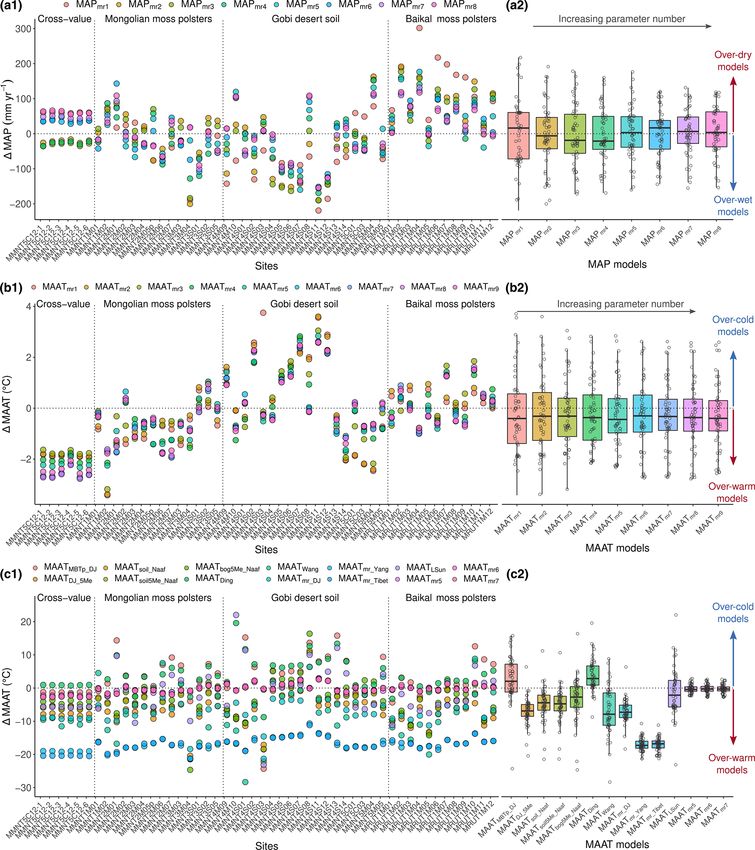
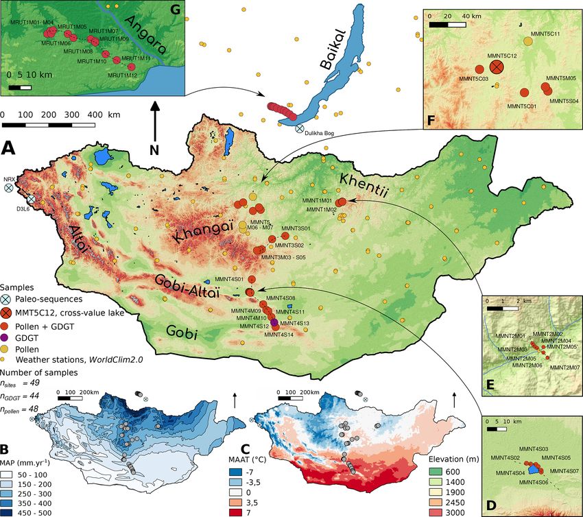
L. Dugerdil et al.: brGDGTs and pollen calibrations for cold–dry environments                                                          1201

Figure 1. (a) Topographic map of Mongolia (from ASTER data) with the location of surface samples and weather stations considered in
the present study; (b) mean annual precipitation; (c) mean annual air temperature; (d) focus on the samples surrounding Taatsiin Tsagaan
Lake, Gobi desert; (e) focus on the samples along a valley in the Khentii range; (f) localization of Khangai surface samples; (g) focus on
the Baikal Lake transect following the Angara valley. The Mongolian GIS data are issued from the ASTER dataset (https://terra.nasa.gov/
about/terra-instruments/aster, last access: January 2018), the meteorological dataset from WorldClim2 and infrastructures from public dataset
(ALAGaC) (https://marine.rutgers.edu/~cfree/gis-data/mongolia-gis-data/, last access: January 2018).

to determine the potential effects of community structure on             to the methylation degree, the ratio of 5-, 6- (De Jonge et
GDGT relative abundances. To evaluate the provenance and                 al., 2013) and 7-methyl isomers (Ding et al., 2016) responds
the climatic information brGDGTs bear, several indexes have              to environment forcing: the 5-methyl brGDGTs mathemat-
been proposed in the literature (Table S1 in the Supplement).            ically correlate mainly with temperature (R 2 = 0.76; Naafs
To monitor these changes, the cyclization ratio of branched              et al., 2017a), while 6- (R 2 = 0.69) and 7-methyl brGDGTs
tetraethers (CBTs) and methylation of branched tetraether                (R 2 = 0.44) seem to correlates with moisture and pH (Yang
(MBT) indexes linked to environmental factors such as cli-               et al., 2015; Ding et al., 2016). More specific indexes have
mate and soil parameters have been proposed (Weijers et                  been proposed by De Jonge et al. (2014a) to limit the multi-
al., 2007b; Huguet et al., 2013). In particular, with regard             correlation systems with the withdrawal of 5-methyl com-

https://doi.org/10.5194/cp-17-1199-2021                                                               Clim. Past, 17, 1199–1226, 2021
1202                                              L. Dugerdil et al.: brGDGTs and pollen calibrations for cold–dry environments

Figure 2. Eurasian map of all the pollen surface samples included in the database. The color code refers to the biome pollen inferred for each
site. The biomes are WAMX, warm mixed forest; WAST, warm steppe; TEDE, temperate deciduous forest; XERO, xerophytic shrubland;
COMX, cool mixed forest; HODE, hot desert; CLMX, cold mixed forest; PION, pioneer forest; TAIG, taiga forest; COST, cold steppe;
COCO, cold conifer forest; TUND, tundra; ANTH, anthropic environment; CLDE, cold deciduous forest; CODE, cold desert. The thickest
points underline the COST samples selected for this study to operate the transfer function method among all COST sites (shown by a lozenge
on map). The arrows indicate the main climatic system driving the Mongolian climate: in orange the Westerlies arriving from the North
Atlantic ocean and in blue the Indian Summer Monsoon (ISM) and the East Asian Summer Monsoon (EASM). The dashed line represents
the EASM limit following Chen et al. (2010), Q. Li et al. (2018) and Haoran and Weihong (2007) for the northernmost part of the boundary.
The Mongolian Plateau (MP) is highlighted by the brown shaded area (Windley and Allen, 1993; Sha et al., 2015). The light blue crossed
circles localize the five cores used as test benches for the calibrations (top-core and paleosequences).

pounds such as MBT05Me , which is independent of the pH,                 quantitative climate reconstruction (Ma et al., 2008), pollen
and CBT5Me which is more representative of the soil pH                   transfer functions (Herzschuh et al., 2003, 2004; Cao et al.,
than the former version of the index (index formula in Ta-               2014; Zheng et al., 2014) and brGDGT regression models
ble S1). The statistical relevance of these indexes is a ma-             (Sun et al., 2011; Yang et al., 2014; Ding et al., 2015; Wang
jor issue in brGDGT calibration (Dearing Crampton-Flood et               et al., 2016; Thomas et al., 2017). Even if all of these stud-
al., 2020). Some regional indexes for soil temperature such              ies focus on areas surrounding the EASM line (Fig. 2; Chen
as Index1 (De Jonge et al., 2014a) and Index2 for Chinese                et al., 2010; Q. Li et al., 2018), the understanding of the cli-
soils (Wang et al., 2016) have been explored too, in the con-            mate cells interaction and oscillation over time is still lacu-
text of a strong local calibration demand (Ding et al., 2015;            nary, and especially on the ACA upper edge. In this con-
Yang et al., 2015). IsoGDGTs were first attributed to lake wa-           text, our study took place in the northernmost part of this
ter column production (Schouten et al., 2012), but they were             climatic system (Haoran and Weihong, 2007). Moreover, we
also described in significant but lower proportions in soils             propose the first multi-proxy calibration exercise in the ACA
(Coffinet et al., 2014). The ratio of isoGDGTs to brGDGTs                area based on pollen and brGDGT fractional abundances re-
(Ri/b ) has been proposed as a reliable aridity proxy (Yang et           trieved from modern samples (soil, moss litter, pond mud)
al., 2014; Xie et al., 2012). It has been shown that a linear            in semiarid to temperate conditions. The aim of this study is
relation exists between these GDGT indexes and some cli-                 to take advantage of new, modern surface sample datasets in
matic features at large regional scales (in the wide Chinese             Baikal area and Mongolia to propose an adapted calibration
biome range, from tropical forest to central arid plateau, for           of pollen and archaeal biomarker proxies for cold and dry en-
instance; Yang et al., 2014; Lei et al., 2016).                          vironments. For that purpose, local calibrations are compared
   Since multi-proxy studies become more and more accu-                  with global calibrations to infer the influence of calibration
rate in both temperature and precipitation reconstruction, lo-           scale and proxy types on derived climatic parameters. Our
cal to regional calibrations have been proposed for dry ar-              approach is summarized in the following steps:
eas such as the arid central Asian (ACA) area: pollen semi-

Clim. Past, 17, 1199–1226, 2021                                                               https://doi.org/10.5194/cp-17-1199-2021
L. Dugerdil et al.: brGDGTs and pollen calibrations for cold–dry environments 1203
1. collection of a new set of modern surface samples for climate models. This core has been clipped into 62 sam-
Mongolia with homogeneous characterization of their ples of which the top-core has been replicated 6 times (sam-
bioclimate environment followed by pollen and GDGT ples MMNT5C12-1 to MMNT5C12-6). Into the MMNT5
pattern characterization; transect, mud from two temporary dry ponds has been sam-
pled. These surface muds are referred in following figures as
2. evaluation of the match between actual bioclimate envi- mud. Into the other transects and depending on aridity and
ronments and the associated pollen rain and biomarker vegetation at each site, a soil or a moss polster was sam-
assemblages based on mathematical criterion without pled. In figures, soil refers to the first 3–5 cm of the ground
eco-physiological considerations; in dry ecosystems, while moss is a mix between soil, litter
and a bryophyte (or Cyperaceae) layer in wetter environ-
3. creation of local Mongolian Plateau (MP) climate cali- ments. Moss acts as a pollen trap recording a 3- to 5-year
brations for pollen and GDGTs and comparison of local mean pollen signal (Räsänen et al., 2004). In drier areas, the
and global calibrations in the Mongolian case study; soil surface samples have the same function, in spite of a
lower pollen conservation and over-representation of some
4. a posteriori validation of the inferred relationships be- taxa (Lebreton et al., 2010). In parallel with the GDGT anal-
tween proxies and ecological likelihood based on the ysis and following the calibration approaches presented in
currently developed evidences of brGDGT and pollen De Jonge et al. (2014a), Davtian et al. (2016) and Naafs et
rain ecological significance; al. (2017a, 2018), mud from temporary ponds and soil sam-
ples as well as the soil part of moss litter were also used for
5. discussion of the implications of the calibration mis- actual GDGT analysis. To summarize, this study is based on
matches in terms of climatic reconstructions in arid and 49 sites, 48 samples in the pollen dataset, 44 in the brGDGT
cold environments; dataset and 6 cross-validation samples to test the brGDGT
models. In terms of sample types, the dataset consists of
6. testing of the new calibrations (pollen and brGDGTs) 30 mosses, 15 soils, 2 pond muds and 2 top-cores.
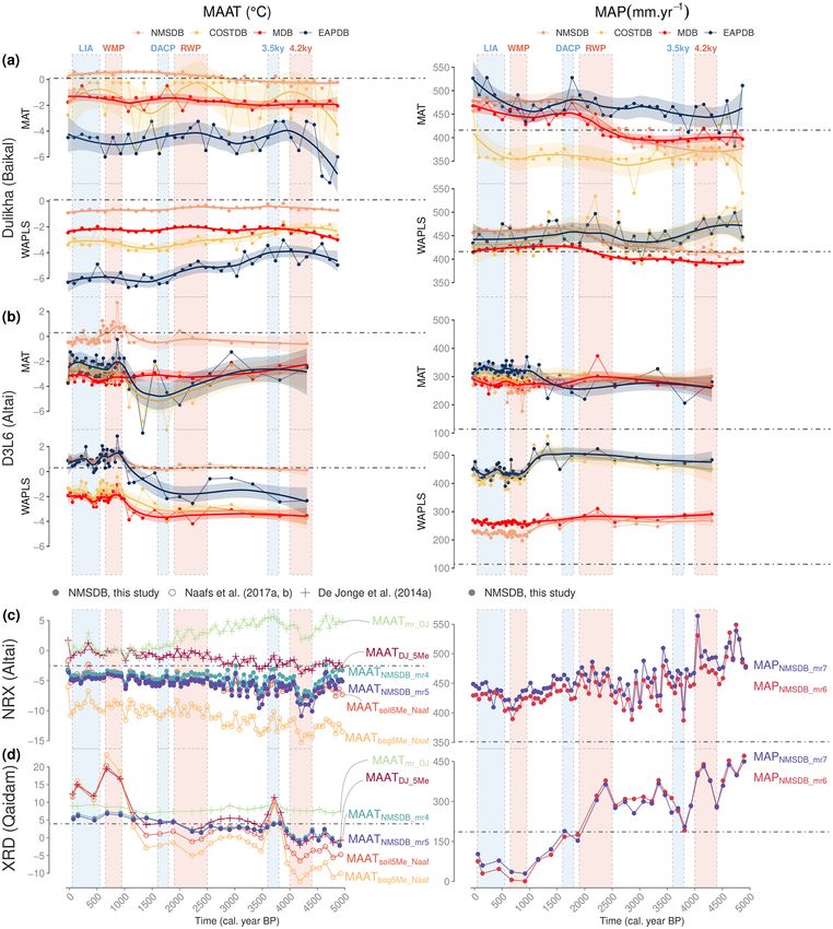
through their application on four surrounding Late To test the reliability of our modern calibrations, we have
Holocene records: two pollen records, Dulikha bog finally selected four paleosequences within or close to the
(Baikal area; Bezrukova et al., 2005; Binney, 2017) and MP used as test benches of the calibrations. For the pollen
Lake D3L6 (Altai; Unkelbach et al., 2019), and two analysis, the cores of D3L6 from Unkelbach et al. (2019)
brGDGT records, NRX (Altai; Rao et al., 2020) and located in the Mongolian Altai range and the Dulikha bog
XRD (Qaidam basin; Sun et al., 2019). (Fig. 1; Bezrukova et al., 2005; Binney, 2017) are com-
pared to the Xiangride section (XRD) used for the brGDGT
sequence from Sun et al. (2019), sampled in the Chinese
2 Mongolian and Baikal study area
Qaidam Basin and the NRX peat bog (Chinese Altai, Fig. 2;
2.1 Coring, sampling area and sample types Rao et al., 2020). These two cores have recorded the pale-
oenvironmental changes of the Late Holocene period.
The study area lies from 52◦ 290 to 43◦ 340 N in latitude and
from 101◦ 000 to 107◦ 060 E in longitude (Fig. 1a). The sample 2.2 Vegetation and biomes
sites (n = 49) are listed in Table S2 with a description of the
sample type, the applied analyses, the coordinates and the as- The central part of the Mongolian Plateau (MP) is charac-
sociated ecosystem. For each site, the Garmin eTreX10 was terized by a dry and cold flat mosaic of steppes and deserts
used to record GPS coordinates to 5 m accuracy. The sur- with a 1220 m a.s.l. median elevation (Fig. 1a; Wesche et al.,
face samples were collected throughout Mongolia in 2016 2016) and is intersected in its northern part by the Sayan and
following four transects (n = 29): in the Khentii mountain Khentii ranges, in its southern part by the Gobi–Altai and
range (MMNT1 and MMNT2; Fig. 1e), in the Orkhon val- Qilian Shan ranges aligned along a NW–SE direction and
ley (MMNT3), and in the Gobi desert and the Gobi–Altai in the west by the Altai range (Windley and Allen, 1993;
range (MMNT4; Fig. 1d). During the same field trip, a fifth Sha et al., 2015). A wet and cold highland in the Khangai
transect has been done in the Sayan range along the Angara ranges culminates at 4000 m a.s.l., and a flatter and wetter
valley, Russia (MRUT1, n = 12; Fig. 1g). A Khangai moun- Mongolian area, the Darkhad basin, is located in the north,
tains field trip from spring 2009 enlarged this set of data close to the Russian border on the edge of the southern
with a sixth transect of surface samples (MMNT5, n = 6, Siberian Sayan range. In the northernmost part of the MP,
in Fig. 1f) and two lake coring samples from Ayrag Nuur the Baikal lake area is characterized by a basin at a lower
(MMNT5C12) and Shargyl Nuur (MMNT5C11), both in altitude (around 600 m a.s.l., Fig. 1g; Demske et al., 2005).
Fig. 1f. Both of these top-cores were added to the surface The distribution of vegetation and biomes follows a lat-
pollen database, while only the MMNT5C12 core has been itudinal belt organization: in the north the boreal forest
used as cross-value to check the accuracy of the brGDGT presents a mosaic of light taiga dominated by Pinus sylvestris
https://doi.org/10.5194/cp-17-1199-2021 Clim. Past, 17, 1199–1226, 2021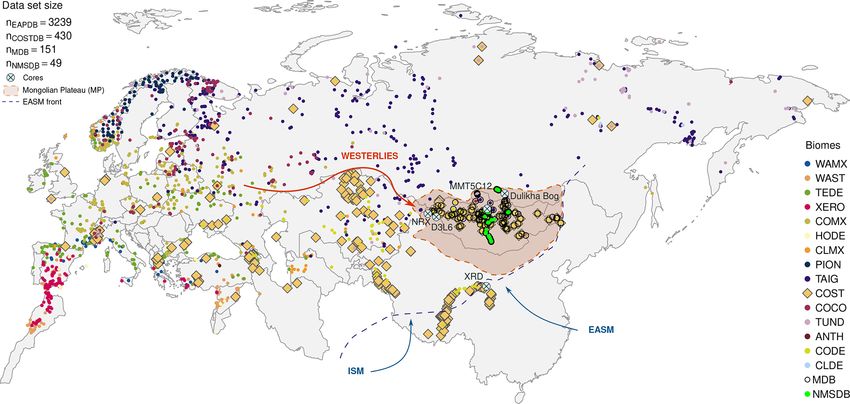
1204                                          L. Dugerdil et al.: brGDGTs and pollen calibrations for cold–dry environments

mixed with riparian forest dominated by birches (Betula           Dulamsuren et al., 2005). However, the precipitation origin
spp.), alders (Alnus spp.) and willows (Salix spp.; Demske        for Mongolia is still under debate (Piao et al., 2018). Mon-
et al., 2005). On the MP, the light taiga dominated by larches    golian summer precipitation up to the Baikal area (Shukurov
(Larix sibirica) and a small amount of birches is mixed with      and Mokhov, 2017) seems to be controlled by the East Asian
dark taiga composed of Siberian pines (Pinus sibirica) and        Summer Monsoon (EASM) system instead of the Westerlies’
spruces (Picea obovata; Dulamsuren et al., 2005; Schlütz          winter precipitation stocked onto the Sayan and Altai range
et al., 2008). The Mongolian taiga is constrained to a re-        (Fig. 2; An et al., 2008). The alternating Westerlies/EASM
gion spanning from the Darkhad Basin to the Khentii range         domination on the MP climate system appears to fluctuate
(Fig. 1a). On the north face of the Khangai piedmont, the         throughout the Holocene depending on the monsoon strength
vegetation is dominated by a mosaic of forest–steppe ecosys-      (Zhang, 2021): the weaker is the monsoon, the further the
tems: the steppe is dominated by the Artemisia spp. associ-       EASM brings precipitation up to the ACA hyper-continental
ated with Poaceae, Amaranthaceae, Liliaceae, Fabaceae and         area. The EASM force may variate in function of the MP
Apiaceae (Dulamsuren et al., 2005). On these open lands           snow cover (albedo effect on sun radiance impact; Liu and
there are some patches of taiga forest, following roughly the     Yanai, 2002) and/or the Pacific surface temperature (Yang
broadside and the northern face of the crest leading on to        and Lau, 1998). Finally, Piao et al. (2018) insist on the im-
the grasslands in the valley (Dulamsuren et al., 2005). The       portance of the locally evaporated water recycling within the
two last vegetation layers in Mongolia through the elevation      Mongolian MAP amount.
gradient are an alpine meadow dominated by Cyperaceae
and Poaceae with a huge floristic biodiversity and an alpine
                                                                  3     Methods
shrubland with pioneer vegetation on the summits (Klinge et
al., 2018). On the southern slope of the range, the ecotone       3.1    Pollen analysis, modern pollen datasets and
between the steppe and the desert vegetation extends hun-                transfer functions
dreds of kilometers from the northern part of the Gobi desert
(with water supplied by the Gobi lake area in between) to the     Different chemical processes were performed on the sam-
Gobi–Altai range in the south (Klinge and Sauer, 2019). In        ples: bryophytic parts of the moss samples were defloccu-
the southernmost part of the country, the warm and dry cli-       lated by potassium hydroxide (KOH) and filtered by 250 and
mate conditions favor desert vegetation dominated by Ama-         10 µm sieves to eliminate the vegetation pieces and the clay
ranthaceae, Nitrariaceae and Zygophyllaceae. The vegetation       particles. Then, acetolysis was performed to destroy biologi-
cover is lower than 25 % and is mainly composed of short          cal cells and highlight the pollen grains. For the soil and pond
herbs, succulent plants and a few crawling shrubs.                mud samples, 2 steps of HCl and HF acid attacks were added
                                                                  to the previous protocol to remove all the carbonate and sili-
2.3    Bioclimate systems
                                                                  cate components. All the residuals were finally concentrated
                                                                  in glycerol and mounted between slide and lamella. The
In the central steppe–forest biome, the vegetation is marked      pollen counts were carried out with a Leica DM1000 LED
by an ecotone with short grassland controlled by grazing in       microscope on a 40× magnification lens. The total pollen
the valley and larches on the slopes. The forest is gathered in   count size was determined by the asymptotic behavior of the
patches constituting between 10 % and 20 % of the total veg-      rarefaction curve. This diagram was plotted during the pollen
etation cover. There are also some patches of Salix and Be-       count using PolSais 2.0, software developed in Python 2.7 for
tula riparian forests among the sub-alpine meadows on the         this study. The rarefaction curve was fitted with a logarithmic
upper part of the range. This vegetation is characteristic of     regression analysis. The counter was suspended whenever
the northern border of the Palearctic steppe biome (Wesche        the regression curve reached a flatter step (Birks et al., 1992).
et al., 2016). This biome is characterized by a range of          A threshold for the local derivation at dx/dy = 0.05 was set.
800 to 1600 m a.s.l., a mean annual air temperature (MAAT;        For each sample, the total pollen count is usually around
Fig. 1c) between −2 and 2 ◦ C, and a mean annual precipi-         n ∈ [350; 500] grains for steppe or forest and n ∈ [250; 300]
tation (MAP; Fig. 1b) from 180 to 400 mm yr−1 (Wesche et          for drier environments such as desert and desert–steppe.
al., 2016 based on Hijmans et al., 2005). In Mongolia, even          Among all of the pollen-inferred climate methods, the
if the MAP is very low (MAPMongolia ∈ [50; 500] mm yr−1 ),        MAT and the WAPLS were applied in this study on four dif-
the major part of the water available for plants is delivered     ferent modern pollen datasets, and on the D3L6 and Dulikha
during late spring and early summer, in contrast to Mediter-      fossil pollen sequence to test the accuracy of these calibra-
ranean and European steppes (Bone et al., 2015; Wesche et         tions (Unkelbach et al., 2019, Figs. 1a and 2). The MAT con-
al., 2016). These seasons are the optimal plant growth peri-      sists of the selection of a limited number of analogue sur-
ods. An unknown amount of precipitation is also brought in        face pollen assemblages with their associated climatic values
winter as snowfall (Rudaya et al., 2020), which is not always     (Guiot, 1990); while the WAPLS uses a weighted average
measured into the weather station MAP. The main part of the       correlation method on a limited number of principal com-
MP MAP occurs during the summer (climate diagrams from            ponents connecting the surface pollen fractional abundance

Clim. Past, 17, 1199–1226, 2021                                                      https://doi.org/10.5194/cp-17-1199-2021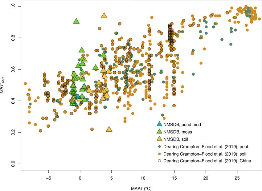
L. Dugerdil et al.: brGDGTs and pollen calibrations for cold–dry environments                                             1205

to the associated climate parameters (ter Braak and Juggins,        quantification. Then, apolar and polar fractions were sep-
1993; Ter Braak et al., 1993). The first dataset, called the        arated on an alumina SPE cartridge using hexane / DCM
New Mongolian–Siberian Database (NMSDB), is composed                (1 : 1) and DCM / MeOH (1 : 1), respectively. Analyses were
of pollen surface samples analyzed in this study (N = 49;           performed in hexane / iso-propanol (99.8 : 0.2) by high-
Figs. 2 and 3). The second one is the same subset aggregated        performance liquid chromatography with atmospheric pres-
to the larger Eurasian Pollen Dataset (EAPDB) compiled by           sure chemical ionization mass spectrometry (HPLC-APCI-
Peyron et al. (2013, 2017). From this dataset of 3191 pollen        MS, Agilent 1200) in the laboratory of LGLTPE-ENS de
sample sites, a pollen–plant-functional-type method was ap-         Lyon, Lyon, following Hopmans et al. (2016) and Davtian
plied to determine the biome for each sample according to the       et al. (2018).
actual pollen rain (Fig. 2; Prentice et al., 1996; Peyron et al.,      Each compound was identified and manually integrated
1998). Then, only the cold steppe (COST) dominant samples           according to its m/z and relative retention time following
were extracted from the main dataset and aggregated with the        the integration descriptions from Liu et al. (2012a), and
NMSDB to produce the COSTDB (N = 430 sites, shown by                De Jonge et al. (2014a) for 5- and 6-methyl brGDGTs and
a lozenge in Fig. 2). Finally, a scale-intermediate dataset of      Ding et al. (2016) for 7-methyl brGDGTs (the peak chro-
samples located within the Mongolian border merged with             matogram integration is displayed in Fig. S1 in the Sup-
the new Mongolian dataset is presented as MDB (N = 151              plement). Statistical treatments on isoGDGT (Fig. 4a) and
sites). The relation between each taxon and climate param-          brGDGT (Fig. 4b) abundances were treated following two
eter was checked and then the MAT and WAPLS methods                 methods presented in Deng et al. (2016), Wang et al. (2016)
were applied with the Rioja package from the R environment          and Yang et al. (2019): compounds were gathered by chemi-
(Juggins and Juggins, 2019).                                        cal structures such as cycles (CBT) or methyl groups (MBT;
                                                                    De Jonge et al., 2014a). brGDGTs were expressed as frac-
3.2   GIS bioclimatic data
                                                                    tional abundance [xi ] (Fig. 4b; Sinninghe Damsté, 2016), as
                                                                    follows:
Because Mongolia and Siberia have relatively few weather                          ni
stations (Fig. 1a), climate parameters were extracted with R        f [x]i =             .                                   (1)
                                                                              NbrGDGT
from the interpolated climatic database WorldClim2 (Fick
                                                                                P
                                                                                      xj
and Hijmans, 2017). We used mean annual precipitation                         j =1
(MAP; Fig. 1b) and mean annual air temperature (MAAT;
Fig. 1c), as well as temperatures and precipitation for spring,        To infer temperatures from brGDGT abundances, two
summer and winter (Tspr , Pspr , Tsum , Psum , Twin and Pwin );     types of model were applied: linear relationships between
mean temperature of the coldest month (MTCO); and the               temperature and MBT–CBT indexes, and multiple regres-
mean temperature of the warmest month (MTWA) in this                sion (mr) models between one climate parameter and a
study to characterize the actual climate. Because the Mon-          proportion of multiple brGDGT fractional abundances. For
golian Plateau is poor in weather stations, the WorldClim2          the simple linear regression model, a correlation matrix be-
database suffers from interpolation errors. The surface sites       tween climate parameters and indexes was calculated us-
presenting inconsistent climate parameters (MAP < 0 or              ing the corrplot Rcran library. For mr models, we devel-
MAP < season precipitation) were removed from the global            oped in the R environment a stepwise selection model (SSM;
database. The elevation data and the topographic map origi-         Yang et al., 2014) to determine the best-fitting model con-
nate from the ASTER imagery (Fig. 1a). The biome type for           necting climate parameters with brGDGT fractional abun-
each site derives from the LandCover database (Olson et al.,        dances. Then we gathered some of the climate–GDGT lin-
2001), classification and field trip observations.                  ear relations established in previous studies (De Jonge et
                                                                    al., 2014a; Naafs et al., 2017a, b, 2018; Sinninghe Damsté,
3.3   GDGT analysis and calibrations                                2016; Yang et al., 2014, 2019) focusing on a single climatic
                                                                    parameter, MAAT (Table S1). These models were clustered
For consistency with the sampling process and the model-            into three categories, by sample type (mosses, soils or pond
ing methodologies developed for pollen analysis, soil parts         muds), geographical area (regional or worldwide scale) and
of the moss polsters, soil samples and pond mud were treated        the statistical model (MBT-CBT based on multiple regres-
for GDGT analysis. After freeze drying, about 0.6 g of mate-        sion models). According to the type of environment from
rial was sub-sampled. The total lipid extract (TLE) was mi-         which the samples originated, there was peat, soil and lake-
crowave extracted (MARS 6 CEM) with dichloromethane                 inferred modeling. All these models were applied to the
(DCM) / MeOH (3 : 1) and filtered on empty SPE car-                 Baikal area–Mongolian surface samples, compared with the
tridges. The extraction step was processed twice. Following         actual MAAT value at each site and applied to the brGDGT
Huguet et al. (2006), C46 GDGTs (GDGTs with two glyc-               XRD section (Fig. 2; Sun et al., 2019) and the NRX bog
erol head groups linked by C20 alkyl chain and two C10              (Figs. 1a and 2; Rao et al., 2020).
alkyl chains) were added as internal standard for GDGT

https://doi.org/10.5194/cp-17-1199-2021                                                      Clim. Past, 17, 1199–1226, 2021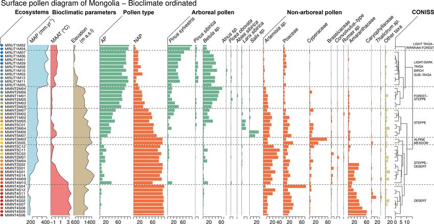
1206                                              L. Dugerdil et al.: brGDGTs and pollen calibrations for cold–dry environments

Figure 3. Simplified surface pollen diagram, bioclimatically sorted, of the Siberian–Mongolian transect. The pollen taxa are expressed in
% TP. The ecosystem units were determined with a CONISS analysis. The left-hand colored dots represent the ecosystem for each sample
from light-taiga–riparian forest (deep blue), light/dark taiga–birch sub-taiga, steppe–forest, alpine meadow, steppe, steppe–desert and desert
(deep red). The color scale is presented in Fig. 5. The MAP and MAAT are extracted from Fick and Hijmans (2017).

Figure 4. Fractional abundances of (a) isoGDGTs and (b) brGDGTs for moss polsters (green), soil surface samples (orange) mud from
temporary dry ponds (blue) and the full sequence of the Lake MMNT5C12 as paleo-brGDGTs comparison (grey). The punctuation marks 0
and 00 refer to 6- and 7-methyl, respectively.

3.4    Statistical analyses                                              elevation, location and soil features) by the way of a re-
                                                                         dundancy analysis (RDA). The regression models were run
GDGTs and pollen data were analyzed with a principal com-                with the p value < 0.05 (model relevance), the R 2 (correla-
ponent analysis (PCA) to determine the axes explaining the               tion level between the variables), the root mean square devia-
variance within the samples. The biotic values (pollen and               tion (RMSE, error on parameter reconstruction) and Akaike’s
GDGTs) were also compared to abiotic parameters (climate,                information criterion (AIC, effect of over-parameterization

Clim. Past, 17, 1199–1226, 2021                                                               https://doi.org/10.5194/cp-17-1199-2021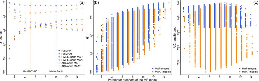
L. Dugerdil et al.: brGDGTs and pollen calibrations for cold–dry environments 1207
on multiple regression models; Arnold, 2010; Symonds and 7. desert dominated by Amaranthaceae (from 25 % to
Moussalli, 2011). A cross-validation test was performed for 65 %) and by rare pollen-type Caryophyllaceae, Thal-
all the brGDGT calibrations (from this study and from the ictrum spp., Nitraria spp. and Tribulus spp.
literature) using an independent set of six lacustrine sam-
ples from the lake MMNT5C12 top-core. Statistical analyses
were performed with the Rcran project, using the ade4 pack- 4.1.2 Pollen–climate interaction
age (Dray and Dufour, 2007) for multivariate analysis. All The pollen rain trends follow similar variations to biocli-
the plots were made with the ggplot2 package (Villanueva mate parameters in MAP, MAAT and elevation (Fig. 3).
and Chen, 2019) or the Rioja package (Juggins and Juggins, The highest AP values are correlated to large MAP (up
2019) for the stratigraphic plot and the pollen clustering us- to 500 mm yr−1 ) and relatively high MAAT (around 1 ◦ C),
ing the CONISS analysis method (Grimm, 1987). in the low-elevation Baikal area. Then the transition be-
tween AP and NAP dominance is marked by decreases in
4 Results both MAAT (−1 ◦ C) and MAP (300 mm yr−1 ) connected to
the high-elevation Khangai range. Finally, the dominance of
4.1 Pollen, climate and ecosystems relations NAP in the Gobi desert area is linked to very arid condi-
tions (MAP < 150 mm yr−1 ) and relatively warm MAAT (up
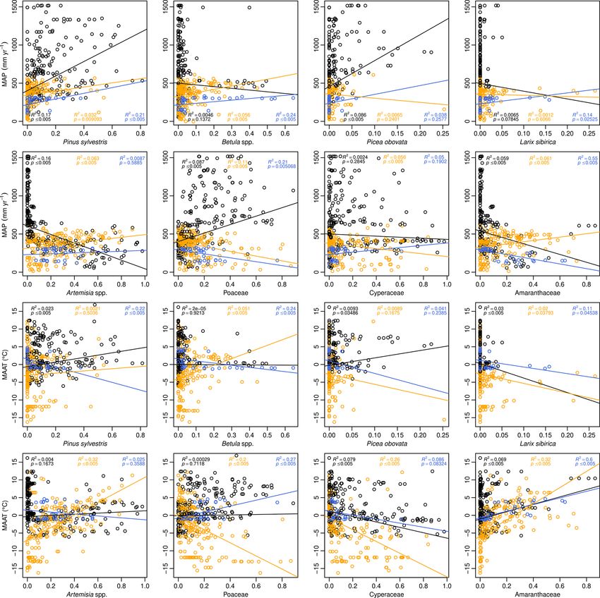
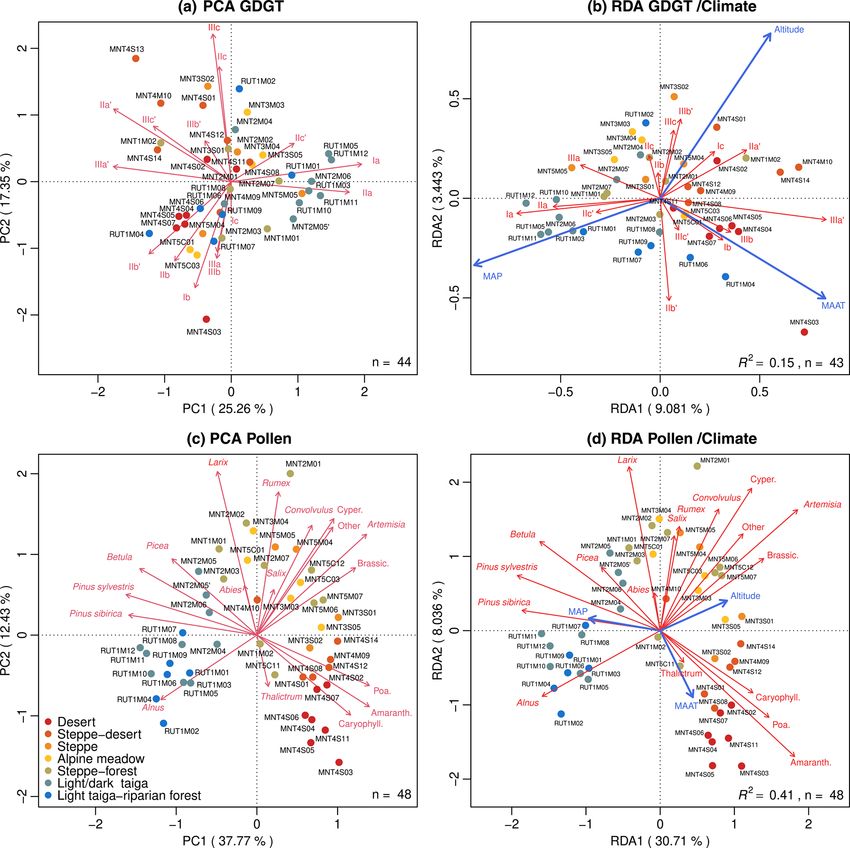
4.1.1 Modern pollen rain and vegetation representation to 4 ◦ C). The correlation between the taxa themselves and
The pollen rain (Fig. 3) is dominated by six main pollen climate parameters is R 2 = 0.38 (RDA; Fig. 5d). The rise in
taxa: Pinus sylvestris, Betula spp., Artemisia spp., Poaceae, MAAT is associated with that of Amaranthaceae, Poaceae,
Cyperaceae and Amaranthaceae. The pollen diagram, sorted Sedum-type and Caryophyllaceae percentages. On the con-
by bioclimate from the wet and relatively warm Baikal area trary, the decrease in MAAT is associated with a rise in the
on the upper part to the dry–warm Gobi desert on the bot- AP and Cyperaceae, Artemisia spp. and Brassicaceae per-
tom, presents a net arboreal pollen (AP) decrease from 85 % centages. MAP, closely related to RDA1 , rises with AP and
to 5 %. A total of 34.26 % of the variance is explained by PC1 decreases with NAP (Fig. 5d). Finally, the elevation gradient
extending from positive values associated with non-arboreal favors Artemisia spp. and Cyperaceae for NAP and Salix spp.
pollen (NAP; Amaranthaceae, Poaceae and Artemisia spp.) and Larix sibirica for AP (Fig. 5d).
to negative values associated with AP (Pinus undet., Betula
spp. Picea obovata and Larix sibirica, in Fig. 5c). This trend 4.1.3 Pollen-inferred climate reconstructions: MAT and
shows the transition between ecosystems, marked by the WAPLS results
seven main CONISS clusters (Fig. 3) and PC1 and PC2 vari-
To reconstruct climate parameters from pollen data, MAT
ations (Fig. 5c). Below are the over-representative main taxa
and WAPLS methods were applied on the four scales, mod-
for each of the Siberian–Mongolian transect ecosystems:
ern pollen datasets and the 10 climate parameters (Table 1).
1. light taiga–riparian forest dominated by Pinus All these methods can be run with n ∈ [1; 10] parameters:
sylvestris (> 70 %), Pinus sibirica and very low NAP the number of analogues for MAT and the number of com-
(< 5 %); ponents for WAPLS. The best transfer functions among all
of them were selected by the following approach: in a first
2. mixed light/dark taiga–birches sub-taiga with an as- step, for each climate parameter the methods fitting with the
semblage of Larix sibirica, Picea obovata, Pinus higher R 2 and the lower RMSE were selected. Then, in case
sylvestris and P. sibirica; the highest R 2 and the lowest RMSE were not applied for
the same number of analogues or components, we chose the
3. forest–steppe ecotone same AP assemblages that the method presenting the lower number of parameters. Despite
light/dark taiga ecosystem with 20 % of Artemisia spp., the small number of parameters relative to the number of
plus occurrence of Poaceae, Cyperaceae, Thalictrum observations, the method fits well (Table 1, Arnold, 2010).
spp. and Convolvulus spp.; MAT method gives better R 2 in bigger DB than in smaller
ones. Fitting increases with the diversity and the size of DB,
4. steppe still dominated by Artemisia spp. (30 %) and ris-
since MAT is looking for the closest value between climate
ing Poaceae (25 %) and Brassicaceae;
and pollen abundance. By contrast, WAPLS fits better on the
5. alpine meadow overpowered by Cyperaceae up to 50 %, local scale and especially with a smaller number of sites. In
Poaceae, Brassicaceae, Amaranthaceae and Convolvu- this case, the pull of data is largest and the variance is largest
lus spp.; (ter Braak and Juggins, 1993). WAPLS also leads to better
values of RMSE than R 2 , in contrast to MAT. For tempera-
6. steppe–desert ecotone highlighting by the transition ture, pollen fits better with Tspr or MTWA in Mongolia. Tem-
between Amaranthaceae–Caryophyllaceae community peratures of the warmest months indeed control both vegeta-
and Poaceae–Artemisia spp. assemblages; tion extension and pollen production (Ge et al., 2017; Li et
https://doi.org/10.5194/cp-17-1199-2021 Clim. Past, 17, 1199–1226, 2021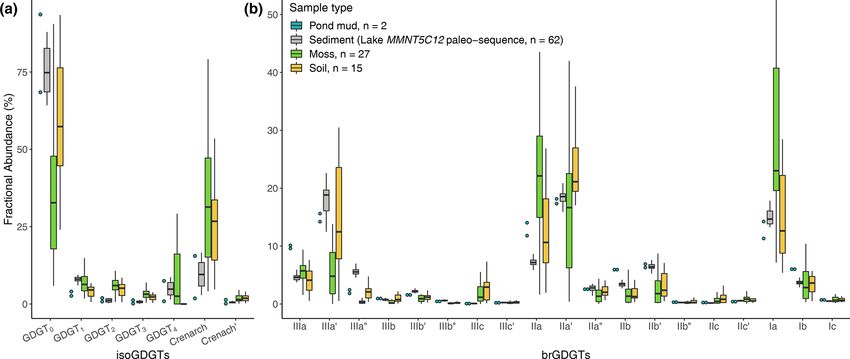
1208                                             L. Dugerdil et al.: brGDGTs and pollen calibrations for cold–dry environments

Figure 5. Multivariate statistics for the proxies clustered by ecosystems: (a) principal components analysis (PCA) and (b) redundancy anal-
ysis (RDA) for brGDGT fractional abundances; (c) PCA and (d) RDA for pollen fractional abundances. The variance percentage explained
is displayed on the axis label; the size of the dataset (n) and the RDA linear regression (R 2 ) are inserted in each plot area.

al., 2011) and especially in very cold areas such as Mongo-             the climate parameters. Even if these two climate parameters
lia. For precipitation, the significant season is the one associ-       are not the best-fitting pollen methods, they are the easiest
ated with the summer monsoon system in Mongolia (Wesche                 to interpret and are comparable with the GDGT regression
et al., 2016). Almost all the Mongolian precipitation falls             models commonly based on MAAT and MAP. In any case,
during the spring and the summer (Wang et al., 2010), and               these models are mitigated by the spatial autocorrelation af-
the amount of precipitation controls, among other parame-               fecting any models made on ecological database (Legendre,
ters, the openness of the landscape in Mongolia (Klinge and             1993) and especially the MAT method more than the WAPLS
Sauer, 2019). To simplify the confrontation of the diverse              (Telford and Birks, 2005, 2011).
models, the MAAT and MAP were isolated from the rest of

Clim. Past, 17, 1199–1226, 2021                                                             https://doi.org/10.5194/cp-17-1199-2021
L. Dugerdil et al.: brGDGTs and pollen calibrations for cold–dry environments 1209
Table 1. Statistical results of the MAT and WAPLS methods applied to four surface pollen datasets and 10 climate parametersa . The lower
number of parameters leading to the best performance is highlighted in bold.
Database Climate WAPLS MAT
parameterb
k best k best k R2 RMSE k best k best k R2 RMSE
R 2c RMSEc selectedd selectedd selectedd R 2c RMSEc selectedd selectedd selectedd
NMSDB MAAT 2 2 2 0.65 1.18 3 13 3 0.58 1.45
(this study) MTWA 2 2 2 0.62 1.69 2 9 2 0.68 1.8
Tspr 2 2 2 0.71 1.26 2 13 2 0.63 1.63
MAP 2 1 1 0.79 61.22 2 6 2 0.88 55.73
Pspr 2 1 1 0.67 11.39 2 4 2 0.89 8.28
Psum 2 2 2 0.8 34.75 2 10 2 0.82 38.49
MDB MAAT 2 1 1 0.35 1.9 5 8 5 0.6 1.65
(Mongolia) MTWA 2 1 1 0.24 2.14 5 9 5 0.53 1.84
MTCO 2 1 1 0.27 2.75 5 7 5 0.66 2.05
MAP 3 1 1 0.23 95.05 9 11 9 0.38 88.73
Psum 1 1 1 0.47 47.02 8 12 8 0.54 46.17
COSTDB MAAT 2 2 2 0.54 4.09 7 10 7 0.73 3.34
(cold steppe) MTWA 3 2 2 0.48 3.55 8 10 8 0.67 3.01
MTCO 2 2 2 0.56 6.34 6 9 6 0.77 4.86
MAP 4 2 2 0.55 224.43 6 9 6 0.77 161.86
Psum 3 2 2 0.34 70.89 5 9 5 0.65 55.08
EAPDB MAAT 3 3 3 0.72 4.08 5 8 5 0.88 2.9
(Eurasia) MTWA 3 3 3 0.55 3.31 5 9 5 0.79 2.5
MTCO 3 3 3 0.72 6.49 4 8 4 0.89 4.46
MAP 3 3 3 0.43 239.6 4 10 4 0.74 181.21
Psum 2 2 2 0.52 62.33 4 8 4 0.8 44.66
a Only the five better-fitting regression models for each climate parameter are shown. b The climate parameters correspond to mean annual air temperature (MAAT), mean temperature of the
warmest (MTWA) and the coldest (MTCO) months, spring temperature (Tspr ), mean annual precipitation (MAP), and precipitation for summer (Psum ) and spring (Pspr ).
c Corresponding to the number of parameters used in the model inferring the best R 2 and RMSE. d Number of parameters, R 2 , RMSE of the finally selected model.
4.2 GDGT–climate calibration ship exists between the crenarchaeol concentration and MAP
(R 2 = 0.14, p value > 0.005). The putative regio-isomer re-
4.2.1 GDGT variance in the dataset sponse to MAP (Buckles et al., 2016) is not evidenced in
NMSDB.
In the MMNT5C12 sediments, isoGDGTs are dominated The average [brGDGT]tot concentrations differ depending
by GDGT-0 and crenarchaeol (74.6 % and 9.8 % in relative on the sample type:
abundances, respectively, in Fig. 4a, grey boxplots). These
compounds, mainly lake-produced (Schouten et al., 2012), [brGDGTtot ]sed = 25.8 ± 8.1 ng g−1
sed ,
are also present in the moss samples (32.7 % and 31.3 %,
[brGDGTtot ]moss = 23.2 ± 26.8 ng g−1
moss ,
green boxplots) and in soils (57.4 % and 26.7 %, orange box-
plots). The variations of their fractional abundance in our soil [brGDGTtot ]soil = 0.3 ± 0.14 ng g−1
soil ,
and moss polster dataset are discrete and poorly linked to [brGDGTtot ]all = 16.7 ± 23.6 ng g−1 (2)
sample .
climate parameters (Fig. 4a). IsoGDGT patterns in lake sed-
iments do not really diverge from soil samples which can brGDGT fractional abundances are consistent with each
lead to postulation that the in situ production of isoGDGTs sample type: the predominant compounds are the Ia , II0a , IIa
in shallow and temporary lakes like MMNT5C12 is reduced and IIIa (Fig. 4b). These compounds mostly explain the to-
(Fig. 4a). At least, it may show that the archaeal community tal variance (Fig. 5a). Particularly, the PC1 represents 22.8 %
both in lakes and in soils is dominated by methanogenic Eu- of the total variance and distinguishes two contrasted poles:
ryarchaeota more than Thaumarchaeota (Zheng et al., 2015; the 5-methyl group (mostly with PC1 > −0.3) associated
Y. Li et al., 2018; Besseling et al., 2018). Then, it appears with steppe–forest and forest sites and the 6- and 7-methyl
(Fig. 4a) that the isoGDGTs produced in soils are domi- group on the far negative PC1 values associated with steppe
nated by crenarchaeol in accordance with studies on high and desert sites. Even if the 7-methyl brGDGTs appear to
alkalinity of the soil (Y. Li et al., 2018) linked to the im- have weak significance in the brGDGT variance explana-
pact of aridity (Zheng et al., 2015). However, no relation- tion (Fig. 5a), the surface sample 7-methyl average fractional
https://doi.org/10.5194/cp-17-1199-2021 Clim. Past, 17, 1199–1226, 20211210 L. Dugerdil et al.: brGDGTs and pollen calibrations for cold–dry environments
abundance around 4.6 % is following the normal order of NSSM = 215 = 32 768 models possible for each climate pa-
magnitude (4.3 % in Cameroon lakes and 6.2 % for Chinese rameter. Even the models including some minor compounds
lakes; Ding et al., 2016). ([br]i < 5 %) have been considered since, in the NMSDB,
The sediment samples from the lake MMNT5C12, used brGDGT fractional abundances are more fairly distributed
for past sequence comparison, are more homogeneous than than in the global database, in which few compounds overlap
the surface samples, especially when compared with the the majority of the compounds (Fig. S4b). Indeed, the cumu-
moss polsters that present a wide variability (Fig. 4b). On lative fractional abundance curve (Fig. S4c) is slightly faster
this figure it appears that, globally, soil samples are more rel- in reaching the asymptote line for the world peat (blue curve)
evant analogues to sediments than moss polsters (especially and the world soil (in brown) than in the NMSDB. The world
the [III0a ], [IIa ] and [Ia ] fractions in Fig. 4). This variabil- peat database needs only three brGDGTs to explain more
ity shows an influence of the sample type on brGDGT re- than 85 % of the fractional abundance against more than 10
sponses. On the other hand, sample type also supports first- compounds in the NDMSDB soils. Then, the better-fitting
order climate and environment information, since soil and equations (with low RMSE and AIC and high R 2 ) were se-
moss polsters originate mainly from steppe to desert envi- lected for each number of parameters (number of brGDGTs
ronments and forest/alpine meadows, respectively. About the issued in the linear regression) for both MAAT and MAP.
pond mud samples, the BIT and IIIa /IIa indexes (Fig. S2) Within the 15 models (one model for each parameter addi-
show that a coherent soil origin is leading the brGDGT input tion), the 9 more contrasted ones were selected for discus-
instead of a lacustrine one (Pearson et al., 2011; Martin et al., sion (Table S3). The models with the best statistical results
2019a; Cao et al., 2020). were comprised of between 5 to 12 parameters and present
a R 2 ∈ [0.62; 0.76], a RMSE around 1.1 ◦ C or 68 mm yr−1 ,
4.2.2 Climate influence on brGDGT indexes
and an AICMAAT ∈ [149; 156] or AICMAP ∈ [503.8; 503.1].
The earlier a parameter is used in the mr models, the greater
The brGDGT/climate RDA shows that the brGDGT variance is its influence. For both MAATmr and MAPmr models, IIIa ,
is dominated by the MAP as the first component (Fig. 5b: III0a , IIIb and III0b are the most relevant compounds for the
RDA1 = 10.01 %). The negative values show higher pre- climate reconstruction (Table 2) which is consistent with the
cipitation and uncyclized 5-Methyl GDGTs, such as Ia , IIa PCA and RDA observations displayed (Fig. 5a and b). Both
and IIIa , while the lower MAP match with 6- or 7-Methyl the MAATmr models infer a positive contribution of III0a and
GDGTs, such as III0a , II0a and II00a in accordance with De Jonge a negative contribution of IIIa , which confirms these mod-
et al. (2014a). The RDA2 is slightly more connected to els as eco-physiologically consistent with the RDA results.
MAAT as opposed to elevation, also clustering the methy- Moreover, except for II0b , all the compounds positively cor-
lated and cyclized GDGTs to the higher MAAT. As in the relate with MAAT and negatively with MAP, in accordance
pollen-climate response, the elevation is a second driving with the MAP–MAAT anti-correlation. The 1T values clos-
factor not to be neglected. The correlation between rela- est to 0 reveal the best-fitting model on each point (Fig. 7, left
tive abundance of methylated and cyclized brGDGTs with panels). Then, the box plot (Fig. 7, right panels) summarizes
climate parameters was not strong (Weijers et al., 2004; the best-fitting model at a regional scale.
Huguet et al., 2013). All the MBT, MBT’, MBT05Me and CBT,
CBT’, CBT5Me relations with climate parameters were tested
and showed a very low correlation with R 2 ∈ [0.1; 0.35] 5 Discussion
(Fig. S3b). Once the MBT (Fig. S4a) and the MBT05Me in-
dexes (Fig. 6) are compared with the world database (Yang et 5.1 Issues in modeling Mongolian extreme bioclimate
al., 2014; Naafs, 2017; Dearing Crampton-Flood et al., 2019) 5.1.1 Appraisal modeling in arid environments
it appears that the NMSDB set is consistent with known val-
ues instead of a wide sample dispersion. According to Dirghangi et al. (2013) and Menges et
al. (2014), the commonly used brGDGT indexes (MBT
4.2.3 Multi-regression models
and CBT) are not relevant for arid areas with MAP <
500 mm yr−1 because the relation between low soil water
The stepwise selection model (SSM) for climate–brGDGT content and soil brGDGT preservation and conservation in-
modeling was applied only on the 5- and 6-methyl, be- terferes in the brGDGT/climate parameters (Dang et al.,
cause 7-methyl brGDGTs show weak significance in the 2016). The MAAT models based on MBT and MBT’ in-
variance explanation (PCA; Fig. 5a). To guarantee the ho- dexes provide colder reconstructions (Fig. 7c2) as shown by
mogeneity of the calibration, the SSM has been applied on De Jonge et al. (2014a), because arid soils favor 6-methyl
the total surface dataset excluding the two pond mud sam- brGDGTs (by pH raising due to the low weathering effect
ples (even if their GDGT input seems to be validated by of the weak precipitation; Dregne, 1983; Haynes and Swift,
the BIT and IIIa /IIa indexes in Fig. S2). The NSSM differ- 1989) and drive the MBT to decrease towards zero. This ex-
ent combinations of the 15 brGDGT compounds result in plains the colder MAATDing and MAATMBT0DJ reconstructed
Clim. Past, 17, 1199–1226, 2021 https://doi.org/10.5194/cp-17-1199-2021L. Dugerdil et al.: brGDGTs and pollen calibrations for cold–dry environments 1211
Figure 6. MBT05Me –MAAT relation comparison between the NMSDB surface samples and the world peat and soil database (Dearing
Crampton-Flood et al., 2019).
Table 2. Statistical values and equations of the best brGDGT MAATmr and MAPmr models.
Model Formula R2 RMSE AIC
MAATmr4 = 4.5 × 1 − 36.8 × [IIIa ] + 7.3 × [III0a ] − 37.2 × [IIIc ] − 24 × [IIb ] − 5.2 × [Ia ] 0.62 1.2 147.6
MAATmr5 = 4.8 × 1 − 38.5 × [IIIa ] + 7.9 × [III0a ] − 27.3 × [IIIc ] − 3.3 × [II0a ] − 26.3 × [IIb ] 0.66 1.1 149
+8.5 × [II0b ] − 5.6 × [Ia ]
MAPmr6 = −639 + 1617 × [IIIa ] + 3208.9 × [IIIb ] + 768.2 × [IIa ] + 1146.7 × [II0a ] + 2925.4 × [IIb ] 0.73 72.4 502.9
+3735.7 × [II0b ] + 2763 × [IIc ] + 1967.3 × [II0c ] + 1237.1 × [Ia ] − 1367.7 × [Ic ]
MAPmr7 = −502.2 + 1547.9 × [IIIa ] + 2569.8 × [IIIb ] − 2052.8 × [III0b ] + 622.8 × [IIa ] + 958.2 × [II0a ] 0.76 69.2 503.1
+2638.8 × [IIb ] + 3445 × [II0b ] + 2880.4 × [IIc ] + 1949.1 × [II0c ] + 1152.7 × [Ia ]
−1047.1 × [Ib ] − 2156.6 × [Ic ]
values compared to the modern ones. Moreover, the main a little error (RMSE = 1.3 ◦ C) for MAAT and R 2 = 0.89
issue in climate modeling in Mongolia is the narrow rela- and RMSE = 23 mm yr−1 for MAP. Whenever the Baikal
tionship between MAAT and MAP. Because of the climatic area–Mongolian calibrations are used for paleoclimatic re-
gradient from dry deserts in the southern latitudes to wet constructions, the RMSE of the climate parameters has to be
taiga forests in the northern ones, MAAT and MAP maps are added to the RMSE model. Moreover, the relevance of the in-
strongly anti-correlated (Figs. 1b, c and S5). If this correla- terpolation models suffers from the transition threshold made
tion is not statistically determined on the range of the global in Mongolia between the EASM and the Eurasian Westerlies
database (R 2 = 0.35, p < 0.005), the impact is significant (Fig. 2; An et al., 2008) and reinforced by the topographic
on the range of the Mongolian sites (R 2 = 0.91, p < 0.005). break (Fig. 1a). Because the mr–GDGT models have been
This correlation could be a bias resulting from the interpo- compiled with the group of Baikal sites which are out of the
lation method of the WorldClim2 database. In fact, there MAAT–MAP strong auto-correlation range (Fig. S5), the re-
are very few weather stations (Fig. 1a; Fick and Hijmans, liability of the independence of the MAAT and MAP models
2017), and their distribution on the large MP is interrupted seems to be guaranteed.
by mountain ranges. According to Fick and Hijmans (2017) The topographic fence in Mongolia also affects the pollen
the interpolation model used in the ACA area(which includes and brGDGT distributions by itself, as seen in both RDA
our study area) gives a strong correlation (R 2 = 0.99) and analyses (Fig. 5b and d) where elevation appears to be a
https://doi.org/10.5194/cp-17-1199-2021 Clim. Past, 17, 1199–1226, 20211212 L. Dugerdil et al.: brGDGTs and pollen calibrations for cold–dry environments Figure 7. Validation of brGDGT-climate models on the study sites: reconstructed values for literature MAAT (a), NMSDB mr–MAAT (b) and MAP (c). Models are tested on the NMSDB sites (1) and the box-plot statistics (2) are provided. Sites are clustered in four groups: cross-value on the six first samples of the independent core MMNT5C12, Arkhangai; moss polsters from Mongolian steppe–forest; Gobi steppe–desert soil samples; and moss polsters from Baikal area. Values are plotted in anomaly. Clim. Past, 17, 1199–1226, 2021 https://doi.org/10.5194/cp-17-1199-2021
L. Dugerdil et al.: brGDGTs and pollen calibrations for cold–dry environments                                               1213

major ecophysiological parameter. Elevation affects vegeta-       2019), the summer mr models are not significantly improv-
tion and pollen rain not just because of its influence on lo-     ing the calibration compared to the MAATmr ones. For in-
cal MAAT and MAP but also because it drives other eco-            stance, the best Tsummr is selected by its AIC, and Tsummr6 is
physiological parameters such as O2 concentration, wind in-       inferred using 6 brGDGTs’ fractional abundance (R 2 = 0.63
tensity, slopes and creeping soils, snow cover, and exposure      and RMSE = 1.53 ◦ C). This lack of seasonality effect, ex-
(Stevens and Fox, 1991; Hilbig, 1995; Klinge et al., 2018).       pected in such cold areas, is consistent with temperate Chi-
Elevation as one of the main brGDGT drivers could also be         nese sites (brGDGT reconstructions; Lei et al., 2016).
explained by the archaeal community responses to pH, mois-
ture and soil compound variations along the altitude gradient     5.1.3   Extreme bioclimatic condition modeling lead to a
(Laldinthar and Dkhar, 2015; Shen et al., 2013; Wang et al.,              better global climate understanding
2015) and the vegetation shifts (Lin et al., 2015; Davtian et
al., 2016; Liang et al., 2019). In any case, a better under-      To reduce the signal / noise ratio, a wider diversity of sam-
standing of the archaeal community’s response to ecophysi-        ple sites should be added as initial inputs in the models.
ological parameter variations will considerably improve the       This raises the question of the availability of reliable sam-
brGDGT calibration process (Xie et al., 2015; Dang et al.,        ples in desert areas. The soil samples in the steppe to desert
2016; De Jonge et al., 2019).                                     biomes are often very dry, and these over-oxic soil conditions
                                                                  are the worst for both pollen preservation (Li et al., 2005;
5.1.2   Particularity of the southern-Siberian–Mongolian
                                                                  Xu et al., 2009) and GDGT production (Dang et al., 2016).
        climate system
                                                                  brGDGT concentrations in moss polsters and temporary dry
                                                                  pond muds are thus higher than in soils in our database (Eq. 2
Both GDGT and pollen calibrations show that the precipita-        and Fig. 4). The explanation of the signal difference between
tion calibrations are more reliable than temperature ones (Ta-    the three types of samples could also originate from the in
bles 1 and 2, Figs. 3, 8 and 7), reflecting that the southern-    situ production of brGDGTs inside the moss predominant
Siberian–Mongolian system seems to be mainly controlled           over the wind-derived particles brought to the moss net. As
by precipitation. This dominance of precipitation could be        well as this, it seems that the pool of moss polster is asso-
due to seasonality. Even if the brGDGT production is consid-      ciated with a similar trend to the worldwide peat samples
ered to be mainly linked to annual temperature means (Wei-        from Naafs et al. (2017b) (Figs. 6 and S4a). Moreover, in the
jers et al., 2007a, b; Peterse et al., 2012), the high-pressure   steppe or desert context of poor availability in archive sites,
Mongolian climate system (Zheng et al., 2004; An et al.,          the edge clay samples or top-cores of shallow and tempo-
2008) favors a strong seasonal contrast: almost all the pre-      rary lakes could be a solution for paleosequence studies. The
cipitation and the positive temperature values happen dur-        two pond mud samples of the NMSDB are included within
ing the summer (Wesche et al., 2016). Consequently, for the       the soil–moss trend for all models (Figs. 5 and S4 and S3 in
NMSDB pollen transfer functions, the seasonal parameters          the Supplement). Even if the brGDGT production and con-
such as MTWA, Tsum and Psum better describe the pollen            centrations are different in soils than in lakes due to lake in
variability than MAAT and MAP climate parameters (bet-            situ production (Tierney and Russell, 2009; Buckles et al.,
ter R 2 and RMSE in Table 1). The opposite is found for           2014), this effect is a function of the lake depth (Colcord et
EAPDB and COSTDB models and calibrations made on                  al., 2015) and consequently negligible for shallow lakes, and
large-scale databases. The Mongolian permafrost persists for      almost absent for lake edge samples as shown by Birks, H. J.
half of the year in the northern part of the country (Sharkhuu,   B. (2012) for Lake Masoko in Tanzania.
2003) and acts on vegetation cover and pollen production             The soils of the Gobi desert also have a high salinity level
(Klinge et al., 2018). Furthermore, the effects of frozen soils   which is also a parameter of control on brGDGT fractional
on soil bacterial communities and GDGT production are             abundances (Zang et al., 2018). This taphonomic bias (also
thought to be important (Kusch et al., 2019) since the ar-        climatically induced) could explain part of the histogram
chaeal community seems to be shifting with abrupt temper-         variance of Fig. 4 related to the sample type as well as the
ature modifications (De Jonge et al., 2019). This seasonal-       shift of the soil cluster from the regression line in the cross-
ity leads to a quasi-equivalence between MAP and PSum (if         value plot of brGDGT MBT’/CBT models in Fig. S3 in the
Pwin ≈ 0 then MAP ≈ Psum ) while MAAT is torn apart by            Supplement. Even if the impact of salinity on sporopollenin
the large TSum − Twin contrast (because the MAAT is an av-        is not well understood, salt properties may affect pollen con-
erage value and not a sum as for MAP). The mathematical           servation in soils (Reddy and Goss, 1971; Gul and Ahmad,
consequences of the seasonality on these two climate pa-          2006).
rameters are not the same. Finally, the MAP appears to be            Finally, the saturation effect of the proxies when they reach
the most reliable climate parameter for southern-Siberian–        the limits of their range of appliance is also to be taken into
Mongolian climate studies according to the NMSDB sites            consideration. Since both pollen and brGDGT signals are
(with MAAT < 5 ◦ C). Even if the brGDGTs seem to respond          analyzed in fractional abundance (i.e., percentage of the to-
to summer temperature (Wang et al., 2016; Kusch et al.,           tal count of concentration), these proxies evolve in a [0; 1]

https://doi.org/10.5194/cp-17-1199-2021                                                      Clim. Past, 17, 1199–1226, 2021
You can also read