UCLA UCLA Electronic Theses and Dissertations - eScholarship
←
→
Page content transcription
If your browser does not render page correctly, please read the page content below
UCLA
UCLA Electronic Theses and Dissertations

Title
Beating the Book: A Machine Learning Approach to Identifying an Edge in NBA Betting
Markets

Permalink
https://escholarship.org/uc/item/115957mb

Author
Dotan, Guy

Publication Date
2020

Peer reviewed|Thesis/dissertation

 eScholarship.org                                Powered by the California Digital Library
                                                                 University of California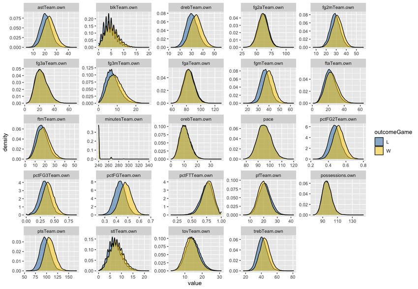
UNIVERSITY OF CALIFORNIA
                Los Angeles

            Beating the Book:
A Machine Learning Approach to Identifying
     an Edge in NBA Betting Markets

 A thesis submitted in partial satisfaction
     of the requirements for the degree
       Master of Applied Statistics

                    by

                Guy Dotan

                   2020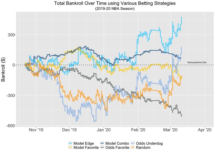
c Copyright by
 Guy Dotan
    2020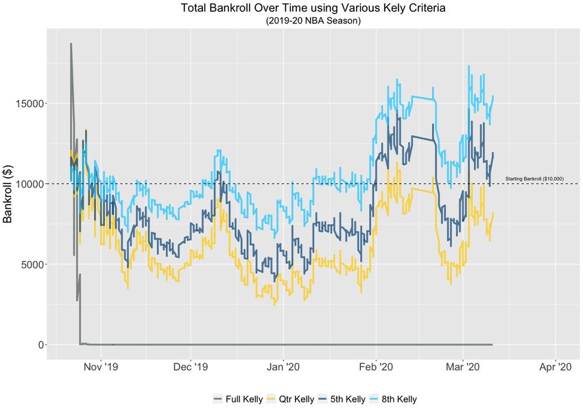
ABSTRACT OF THE THESIS

                                      Beating the Book:
                        A Machine Learning Approach to Identifying
                             an Edge in NBA Betting Markets

                                              by

                                         Guy Dotan
                                Master of Applied Statistics
                         University of California, Los Angeles, 2020
                       Professor Frederic R. Paik Schoenberg, Chair

With the recent rise of sports analytics, legalization of sports gambling, and increase in data
availability to the everyday consumer, the opportunity to close the gap between the bettor
and the casino appears more attainable than ever before. Our hypothesis was that one could
build a model capable of exploiting the inherent inefficiencies that might exist within the
betting marketplace.

   Part one of this study required a derivation of the mathematics behind betting odds to
determine the true probability a sportsbook places on the outcome of a matchup. Integral
to this analysis was to factor in the casino’s always-included cut of the betting pool (known
as the “vig”) that are baked into all wagers to maximize profits.

   Part two was the model building process in which we trained on an archive of team-level,
NBA box scores dating back to 2007 in order to predict which team in the matchup would
win or lose. We aggregated our pace-adjusted box score metrics using two different method-
ologies, rolling eight-game spans and accumulated year-to-date statistics, and then applied
these datasets to four different modeling implementations: logistic regression, random forest,
XGBoost, and neural networks. Our results were optimistic, as all models were able to ac-
curately predict the winner of a matchup at a rate of greater than 60%, thus outperforming
random chance.

                                              ii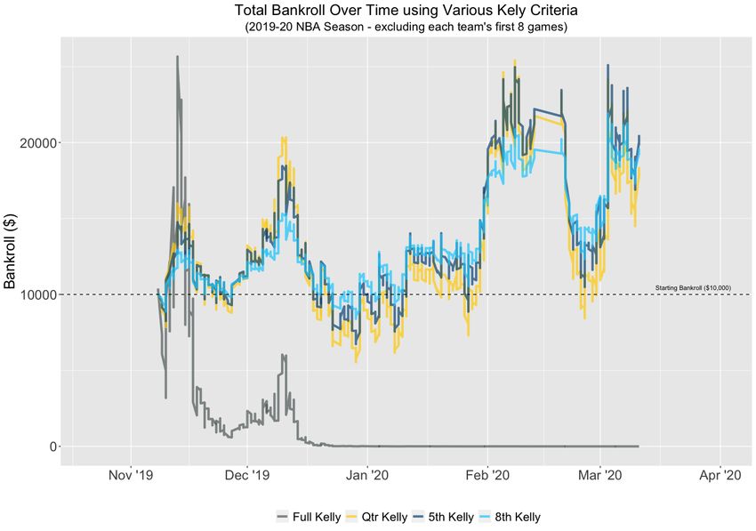
The final part of this research involved seeing how our best model faired versus the real-
world betting lines for the 2019-20 NBA season. We used our logistic model to get a win
probability for each team in every matchup and compared that result to the probability as
defined by the sportsbook odds. This betting edge (the discrepancy between our model and
the sportsbook) was used in a variety of betting strategies. Using our best fixed wagering
technique, we were able to generate a return on investment of about 5% over the course of the
entire season. Using a more complicated wagering method known as the Kelly criterion—a
strategy that adjusts the amount of money wagered based on the size of the edge identified—
we were able to almost double our investment with a return of about 98%. In summary,
building a betting model to gain a gambling edge was determined to be quite achievable.

                                             iii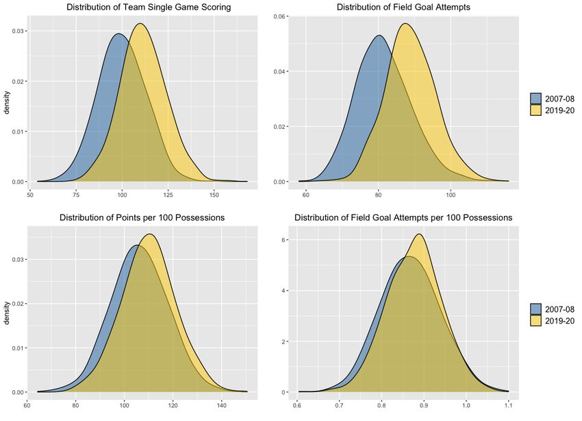
The thesis of Guy Dotan is approved.

                                        Zili Liu

                                       Vivian Lew

                     Frederic R. Paik Schoenberg, Committee Chair

                          University of California, Los Angeles

                                          2020

                                           iv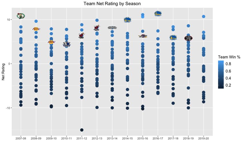
Dedicated to my parents . . .
             for never losing faith that their favorite son, who,
          growing up, would waste his time checking box scores,
        playing fantasy sports, and reading electoral college maps,
                       would eventually find his way.

...also Steph Curry, for bringing basketball back to the Bay Area. Big time.
                            #strengthinnumbers

                                      v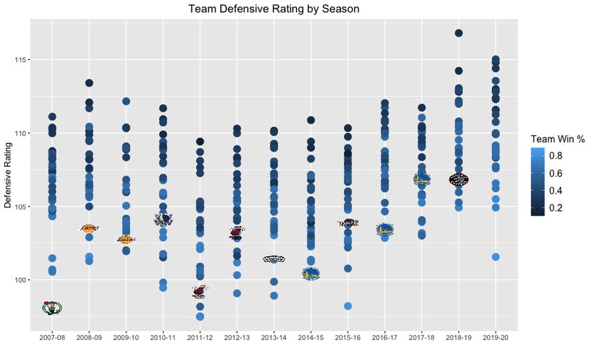
TABLE OF CONTENTS

1 Introduction . . . . . . . . . . . . . . . . . . . . . . . . . . . . . . . . . . . . . .       1

   1.1   Current State of Sports Analytics . . . . . . . . . . . . . . . . . . . . . . . .       1

   1.2   The Legalization of Sports Gambling . . . . . . . . . . . . . . . . . . . . . .         2

   1.3   The Intersection of Data and Wagering . . . . . . . . . . . . . . . . . . . . .         3

2 The Mathematics of Sports Gambling . . . . . . . . . . . . . . . . . . . . .                   6

   2.1   Point Spreads, Totals, and Moneylines . . . . . . . . . . . . . . . . . . . . .         6

   2.2   Implied Win Probability . . . . . . . . . . . . . . . . . . . . . . . . . . . . .       9

   2.3   Derivation of Implied Win Probability . . . . . . . . . . . . . . . . . . . . .         9

   2.4   The Vig or the Juice . . . . . . . . . . . . . . . . . . . . . . . . . . . . . . .     11

   2.5   “Removing the Juice” - Actual Win Probability . . . . . . . . . . . . . . . .          13

3 Data Collection . . . . . . . . . . . . . . . . . . . . . . . . . . . . . . . . . . . .       14

   3.1   Betting Lines . . . . . . . . . . . . . . . . . . . . . . . . . . . . . . . . . . .    15

   3.2   NBA Game Statistics . . . . . . . . . . . . . . . . . . . . . . . . . . . . . . .      16

   3.3   Advanced Metrics . . . . . . . . . . . . . . . . . . . . . . . . . . . . . . . . .     18

4 Data Processing and Exploratory Analysis                . . . . . . . . . . . . . . . . . .   20

   4.1   Seasonal Trends . . . . . . . . . . . . . . . . . . . . . . . . . . . . . . . . . .    20

   4.2   Adjusting for Pace . . . . . . . . . . . . . . . . . . . . . . . . . . . . . . . .     22

   4.3   Aggregation . . . . . . . . . . . . . . . . . . . . . . . . . . . . . . . . . . . .    26

5 Model Building . . . . . . . . . . . . . . . . . . . . . . . . . . . . . . . . . . . .        29

   5.1   Logistic Regression . . . . . . . . . . . . . . . . . . . . . . . . . . . . . . . .    31

   5.2   Random Forest . . . . . . . . . . . . . . . . . . . . . . . . . . . . . . . . . .      35

                                               vi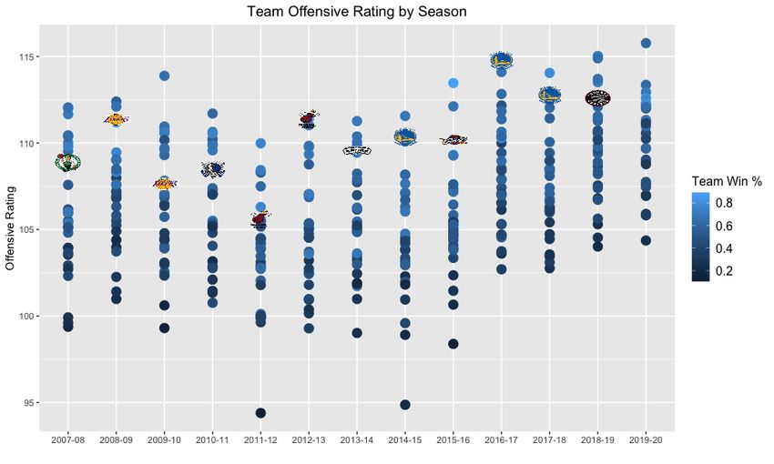
5.3   XGBoost . . . . . . . . . . . . . . . . . . . . . . . . . . . . . . . . . . . . . .   37

   5.4   Modeling Summary . . . . . . . . . . . . . . . . . . . . . . . . . . . . . . . .      39

6 Neural Networks . . . . . . . . . . . . . . . . . . . . . . . . . . . . . . . . . . .        43

   6.1   Basic Structure and Theory . . . . . . . . . . . . . . . . . . . . . . . . . . .      43

   6.2   Model Processing and Results . . . . . . . . . . . . . . . . . . . . . . . . . .      44

7 Beating the Book . . . . . . . . . . . . . . . . . . . . . . . . . . . . . . . . . .         48

   7.1   Why 52.4% Matters . . . . . . . . . . . . . . . . . . . . . . . . . . . . . . . .     48

   7.2   Fixed Bet Implementation . . . . . . . . . . . . . . . . . . . . . . . . . . . .      51

   7.3   Betting Results on the Validation Set . . . . . . . . . . . . . . . . . . . . . .     52

8 The Kelly Criterion . . . . . . . . . . . . . . . . . . . . . . . . . . . . . . . . .        56

   8.1   Deriving the Kelly Criterion . . . . . . . . . . . . . . . . . . . . . . . . . . .    57

         8.1.1   The Compounding Bankroll Model . . . . . . . . . . . . . . . . . . .          57

         8.1.2   Compounding Growth Rate . . . . . . . . . . . . . . . . . . . . . . .         59

         8.1.3   Maximizing growth rate . . . . . . . . . . . . . . . . . . . . . . . . .      59

         8.1.4   An example application of the Kelly Criterion . . . . . . . . . . . . .       61

   8.2   Applying the Kelly Strategy to our Data . . . . . . . . . . . . . . . . . . . .       63

9 Conclusion . . . . . . . . . . . . . . . . . . . . . . . . . . . . . . . . . . . . . . .     69

   9.1   Further Research . . . . . . . . . . . . . . . . . . . . . . . . . . . . . . . . .    69

   9.2   Final Thoughts . . . . . . . . . . . . . . . . . . . . . . . . . . . . . . . . . .    71

10 Appendix . . . . . . . . . . . . . . . . . . . . . . . . . . . . . . . . . . . . . . .      73

References . . . . . . . . . . . . . . . . . . . . . . . . . . . . . . . . . . . . . . . . .   77

                                               vii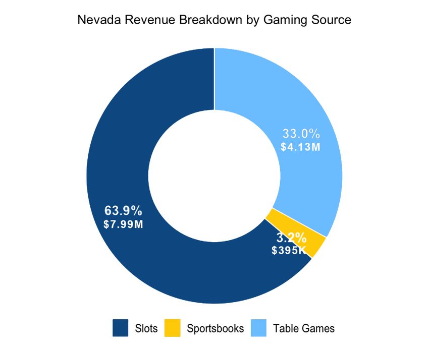
LIST OF FIGURES

1.1   U.S. map of the current state of sports gambling legislation (as of May 2020). .           3

1.2   Total gaming revenue by the source in Nevada from Mar. 2019 to Feb. 2020. . .              4

3.1   2017 survey from Gallup on Americans and their favorite sport to watch. . . . .           14

4.1   Statistical trends by season. . . . . . . . . . . . . . . . . . . . . . . . . . . . . .   21

4.2   Team pace by season. . . . . . . . . . . . . . . . . . . . . . . . . . . . . . . . . .    23

4.3   Pace adjusted metrics, 2007-08 vs. 2019-20. . . . . . . . . . . . . . . . . . . . .       24

4.4   Offensive rating by season (NBA champion indicated by team logo). . . . . . . .           25

4.5   Defensive rating by season (NBA champion indicated by team logo).           . . . . . .   25

4.6   Net rating by season (NBA champion indicated by team logo). . . . . . . . . . .           26

5.1   Correlation matrix for box score statistics. . . . . . . . . . . . . . . . . . . . . .    29

5.2   Density distribution matrix for box score statistics. . . . . . . . . . . . . . . . .     31

5.3   Simplified examples of linear regression versus logistic regression. . . . . . . . .      32

5.4   Top variables by importance from both selection methodologies. . . . . . . . . .          34

5.5   Performance of our four different logistic regression models. . . . . . . . . . . . .     35

5.6   Performance of the random forest model on our two aggregation data sets. . . .            36

5.7   Top 20 variables by importance in the year-to-date random forest model. . . . .           37

5.8   Performance of the XGBoost model on our two aggregation data sets. . . . . . .            39

5.9   Top 20 variables by importance in the year-to-date XGBoost model. . . . . . . .           40

5.10 Performance results from all model types and aggregation methods in this study.            41

6.1   Basic diagram of a neural network with three hidden layers. . . . . . . . . . . .         44

6.2   Accuracy of each neural network based on each combination of hyperparameters.             45

                                               viii
6.3 Performance of the neural network model on our two aggregation data sets. . . . 46
7.1 Break-even point based on expected return on investment for a -110 moneyline bet. 50
7.2 Our two fixed bet wagering implementations. . . . . . . . . . . . . . . . . . . . 52
7.3 Bankroll over time for betting results on odds from the 2019-20 NBA season. . . 53
8.1 Bankroll over time using various Kelly criteria for the 2019-20 NBA season. . . . 65
8.2 Results from various Kelly criteria after excluding each team’s first eight games. 67
10.1 Distribution of moneylines for both teams by season from 2007-2020. . . . . . . 74
ixLIST OF TABLES
2.1 Summary of betting values for the sample wager. . . . . . . . . . . . . . . . . . 13
3.1 Data dictionary of variables from betting archive and NBA box scores. . . . . . 17
5.1 Confusion matrix results for the most performant logistic regression. . . . . . . . 35
5.2 Confusion matrix results for the year-to-date random forest model. . . . . . . . 36
5.3 Confusion matrix results for the year-to-date XGBoost model. . . . . . . . . . . 39
5.4 Summary metrics for all model types and aggregation methods on testing dataset. 41
5.5 Extra summary metrics for all models and aggregation methods on test dataset. 42
6.1 Confusion matrix results for the year-to-date neural network model. . . . . . . . 46
7.1 Summary results between fixed betting methodologies. . . . . . . . . . . . . . . 55
8.1 Summary results between our fractional Kelly criteria. . . . . . . . . . . . . . . 66
8.2 Fractional Kelly results after excluding each team’s first eight games. . . . . . . 68
10.1 Record for matchup favorites based on the sportsbook betting odds. . . . . . . . 73
10.2 League average stats per game by season. . . . . . . . . . . . . . . . . . . . . . 75
10.3 Final logistic model from the year-to-date dataset used for betting implementation. 76
xACKNOWLEDGMENTS
First and foremost, I’d like to acknowledge UCLA for the eight memorable years I spent
on this campus. But more specifically, the UCLA Statistics faculty, staff, and community.
I’ll never forget the first time I stumbled into 8th floor of the Math-Sciences building as
an undergrad, distraught over whether I would ever find my academic passion at UCLA.
Fortunately, Glenda Jones was there to great me, support me, and guarantee that she and
the rest of the statistics department had my back. That I was safe to call this place my
home. And she was right.
Next I’d like to thank all of my professors in the MAS program for sacrificing three hours
of their evenings, every week, to teach a bunch of tired professionals after their long day at
work. Your custom-made curriculums designed directly for our interests and work-related
necessities made commuting to class, not a burden, but a privilege. Thank you for your time,
attention, and gracious flexibility with deadlines. Extra special thanks to Rick Schoenberg
and Vivian Lew for their integral contributions to my academic success.
Lastly, I must acknowledge the companies that have filled in all my knowledge gaps and
pushed me further than academics could ever do alone. What I’ve learned in my experiences
at Tixr, STATS, GumGum Sports, and WagerWire has been invaluable and I would not be
where I am personally and professionally without each and every one of them.
And of course, love and thanks to both my brothers, for their mentorship every step of
the way.
xiCHAPTER 1
Introduction
The world of sports analytics has progressed rapidly over the past decade and with these
advances, the entire professional sports landscape has evolved with it. While general ad-
vances in technology and sports organizations’ willingness to pursue analytical research has
facilitated the evolution, two seminal shifts within the field stand out as reasons for this
surge. The first: proliferation and democratization of accessible data. The second, and more
recently: the federal legalization of sports gambling within the United States.
The sports industry is one of the newest sectors to be disrupted by the emergence of
data-driven decision making challenging preconceived notions from “experts,” and its im-
pact has been fast and far reaching. Setting aside the unprecedented shock to the eco-
nomic ecosystem—specifically within sports and entertainment—from the 2020 outbreak
of COVID-19, the sports analytics business has been thriving. “The global sports analytics
market is expected to reach a revenue of $4.5 billion by 2024, growing at a CAGR [compound
annual growth rate] of 43.5%.” [LLP18]
1.1 Current State of Sports Analytics
To the general public, the most well-known adoption of analytics into the sports universe
was within Major League Baseball, thanks largely to Michael Lewis’ 2003 book Moneyball
and subsequent movie blockbuster, starring Brad Pitt, in 2011. The story chronicles the
influence of Bill James, the field of empirical baseball research known as Sabermetrics, and
the story of the 2002 Oakland A’s unlikely success. Moneyball has been the poster child
of how data can create a competitive edge on the playing field. But sports analytics has
1made its impression in far more avenues than just baseball. The field is responsible for the
increased emphasis of the three-point shot in basketball, the use of optical player tracking
technology in the NFL, and even the statistical optimization of curling game strategy that
helped the Swedish women’s national team to a gold medal in the 2018 Winter Olympics
[Her18], just to name a few.
The integration of data analysts and scientists as crucial members of professional sports
organizations appears here to stay, but this acceptance of analytics is not reserved to just
a small circle of experts working for teams. The true acceleration of the movement is due
to the passion from fans enabled by the increased availability of data. The NFL and NBA
hold yearly hackathons to allow anyone the opportunity to dive into their sport’s data and
present findings to top league officials with prizes and networking at stake. Conferences such
as the Sloan Sports Analytics Conference in Boston began as a small gathering of about 100
attendees in 2006, and now, in 2020, attracts over 4,000 people. The conference has gained
national recognition, notably hosting former President Barack Obama as the keynote speaker
in 2018. The industry’s explosion in popularity though, has been aided by communities such
as FiveThirtyEight, Retrosheet, Sports-Reference, and league-offered APIs bestowing data
democracy to anyone that desires. Sports analytics has largely become open-source and this
hive mind has benefited players, teams, franchises, and fans.
1.2 The Legalization of Sports Gambling
On May 14, 2018, the Supreme Court case Murphy v. National Collegiate Athletic Asso-
ciation reached a landmark decision regarding the federal government’s right to control a
state’s ability to sponsor sports betting. In a 6-3 decision, the Professional and Amateur
Sports Protection Act of 1992 (PASPA) was overturned, thus opening the doors for every
state to make its own laws permitting in-state sports wagering.
In just two years since the ruling there are already 18 states with full-scale legalization
and another six that have passed legislation that will take effect in the coming year. [Rod20]
And as one would expect, bettors in legal states have flocked to sportsbooks, both digital
2and brick-and-mortar. (Sportsbooks, or “books”, are places, usually part of a greater casino,
where bettors can make wagers on all types of sporting events.) Since the overturning of
PASPA, Americans have placed over $20 billion of bets which have generated $1.4 billion
of revenue in those legal states. [Leg20] Morgan Stanley projects that in just five years, by
2025, almost three-quarters of US states (36) will have legalized sports betting and the U.S.
market could see $7 to $8 billion in revenue. [AP19]
Figure 1.1: U.S. map of the current state of sports gambling legislation (as of May 2020).
1.3 The Intersection of Data and Wagering
Sportsbook operators within casinos have had decades of experience building a complex in-
frastructure of analytics to help them determine where to set their gambling lines. Their
goal is to establish betting odds in a matchup such that there is an even amount of money
wagered on both sides of the bet. This allows them to take their cut of the wagers (known
in the industry as the “vigorish” or “vig”) and thus drive revenue to their casino, no matter
which team wins. For the entirety of their existence, sportsbooks have maintained a sig-
nificant advantage over the majority of bettors. Their leverage was largely based on their
3access to data and domain expertise, building models to establish the perfect betting line. It
is this statistical edge that keeps income flowing into sportsbooks. Money that helps build
lavish 50-story casinos and hotels that make the Las Vegas strip world-renowned. That said,
surprisingly, sports wagering accounts for just 3% of the gaming revenue in Nevada casinos.
[Boa20]
Figure 1.2: Total gaming revenue by the source in Nevada from Mar. 2019 to Feb. 2020.
But now, with sports wagering becoming more commonplace in American society and
the proliferation of available sports data to everyday consumers, there is an opportunity
to close the gap between casinos and bettors. Similar to how stockbrokers use proprietary
projection models to systematically “beat the market,” sports wagering has followed suit.
It had always been a one-sided battle between the everyday bettor and the house. But in
this digital age of data availability, the barrier to enter has lowered, thus leveling the playing
field. The war between the book and the bettor is now an arms race where the munition is
data, and for the first time in history, it might be winnable for the bettor.
Recall, a sportsbook’s objective on each bet is to account for an even amount of money
wagered on both sides. Oftentimes a betting line is skewed by the inherent biases of an
average sports bettor. For example, if the Los Angeles Lakers (a TV market size of over five
4million people) were to play the San Antonio Spurs (TV market size of just 900 thousand), we
might expect a sportsbook to place the line so it slightly favors the Spurs. Even if the teams
were evenly matched, sportsbooks would anticipate a disproportionate amount of hometown
favorite bets supporting the Lakers. Just the smallest marginal edge, demonstrated by this
example, could be enough to be exploited by an adept model. A model, when applied to a
large enough dataset, could yield a considerable return on investment.
The goal of this study is to determine if applying machine learning methods to vast sports
datasets (in this case, within the NBA) can create such a model that would give a bettor
the competitive edge over the lines set by a sportsbook.
5CHAPTER 2
The Mathematics of Sports Gambling
To understand how to beat the bookmakers, one first needs to understand how to interpret
the betting lines they provide. There is a wide array of different types of bets that a person
can make at a sportsbook. The three most popular betting styles are: “point spreads,”
“totals (over/under),” and “moneylines.” This chapter will go into detail with descriptions
of these types of bets using basketball as an example.
2.1 Point Spreads, Totals, and Moneylines
Point spreads are mechanisms used to account for the discrepancy between two unevenly
matched teams. Usually notated as: Warriors (-5) vs. Clippers or the inverse: Clippers
(+5) vs. Warriors. The number in the parentheses is called the “spread.” Essentially, the
sportsbook believes that the Warriors are more likely to win the game, but the book wants to
drive an even amount of bettors to wager on the Clippers (even though they are underdogs)
as the Warriors. Therefore, the bookmakers suggest placing a spread of five points on the
game. So if you bet on the Warriors, they need to win by more than 5 points for you to win
the bet. If you bet on the Clippers, they have to lose by 4 points or fewer or win the game,
for you to cash in on the wager. If the game ends with the Warriors winning by 5 points,
then this is called a “push” and all bettors get their money back. Sometimes a spread will
be listed at 0 points (called a “pick-em”), indicating that this is an even matchup and all
you have to do is pick the winner to win the bet.
Similar to point spreads, totals (over/under) involve a specific point amount that a bettor
needs to wager on the correct side of. However, in this case, the winner of the game is
6irrelevant. All the bettor must do is guess if the combined score between the teams will be
greater than or less than the line. For example, Warriors vs. Clippers (o200). If you bet
the “over 200”, you are expecting the combined score between the two teams to reach 201 or
more and it does not matter what combination it occurs (Warriors 120-Clippers 81, Clippers
101-Warriors 100, etc.) If the final combined score is exactly 200, again this is called a push
and bettors get their money back. For this reason, totals (and spreads, for that matter),
oftentimes use fractional lines (+5.5 or o200.5) to prevent the case of a push. Over/under
can be offered for single quarters, just the first half, just the second half, or even for a single
team’s score.
The third popular betting type is called “moneylines” and is the subject of this study.
In a moneyline bet, a person simply needs to determine which team will win the game,
regardless of the score. But if one team was the heavy favorite versus the other team, it
would not make sense for a sportsbook to pay out an equal amount for choosing the favorite
as choosing the underdog. As a result, sportsbooks offer a moneyline, which adjusts the
amount you win for having your bet hit based on the likelihood that the team will win the
game. Moneylines are notated in various formats: decimal, fractional, and moneyline. The
first two are commonly used in Europe. This paper will use the moneyline odds notation
since they are most common to the US (and often called “American” odds). Moneylines
are written as follows: Warriors (-235) vs. Clippers, or conversely, Clippers (+185) vs.
Warriors.
Essentially, these either positive or negative numbers imply how much money a bettor
would profit relative to a $100 bet. +185 means that if a bettor laid $100 on the Clippers,
and then they won the game, the bettor would make $185 profit. -235 means that a bettor
would have to wager $235 to profit $100 from that game. So if a bettor placed $100 on the
Warriors at -235 moneyline odds, and the Warriors indeed won, the bettor makes $42.55
profit. Derivations for these two formulas are shown in Equation 2.1 and 2.2.
7Moneyline Profit - Underdog
Let P rof itdog = Πd and M oneyline = M L
ML Πd
=
100 Risk
100 × Πd = M L × Risk (2.1)
ML
Πd = × Risk
100
Using our example...
+185
Πd = × 100
100
= 1.85 × 100
= $185
Moneyline Profit - Favorite
Let P rof itf av = Πf
−M L Risk
=
100 Πf
Πf × (−M L) = Risk × 100 (2.2)
100
Πf = × Risk
(−M L)
Using our example...
100
Πf = × 100
−(−235)
100
= × 100
235
= .4255 × 100
= $42.55
In summary, a $100 bet on the Clippers (+185) leads to $185 profit. A $100 bet on
the Warriors (-235) leads to about $42 profit. This discrepancy in profits is to discourage
enough bettors from taking the favorite Warriors and instead take the potential for upside
in profit by betting on the underdog Clippers. Again, the sportsbooks goal is to optimize
these moneylines to set it at a line such that an even amount of money is placed on both
sides.
82.2 Implied Win Probability
The payout formula for moneylines makes it quite simple to determine how much profit a
bettor can make from having their wager hit. Risk-averse bettors tend to take favorites
(negative moneylines) despite the lower payouts because there is a higher chance that the
team they bet on will win. Risky bettors will seek out underdogs (positive moneylines) with
lower probabilities of winning, but they think will surprise the public, win the game, and
thus provide a larger profit-margin.
In addition to the payout, however, moneylines can be converted into a win probability
known as “implied probability.” The implied probability formula is defined as the size of
the bettor’s wager divided by the return on investment for that wager. Or simply: risk over
return. When placing a wager and consequently winning that wager, the bettor receives
their initial risk amount back in addition to the profit-margin. Thus, return on investment
of a wager is just risk plus return.
Risk
ImpliedP robability = (2.3)
Return
Note: Return = Risk + Profit
2.3 Derivation of Implied Win Probability
A universal formula to calculate the implied win probability for any bet (underdog or favorite)
can be derived by plugging in the formula for moneyline profit for an underdog (Equation
2.1) and a favorite (Equation 2.2) into the implied probability formula (Equation 2.3).
9Implied Probability - Underdog
Risk
IPdog =
Return
Risk
=
Risk + Πd
Risk
=
Risk + M L
100
× Risk
Risk (2.4)
=
Risk 1 + M L
100
1
=
1+ M L
100
100
IPdog =
100 + M L
Implied Probability - Favorite
Risk
IPf av =
Return
Risk
=
Risk + Πf
Risk
= 100
Risk + −M L
× Risk
Risk (2.5)
= 100
Risk 1 + −M L
1
= 100
1 + (−M L)
(−M L)
IPf av =
(−M L) + 100
Implied Probability - General Equation
100
, if ML ≥ 0
M L + 100
IP(ML) = (2.6)
(−M L)
, if ML < 0
(−M L) + 100
102.4 The Vig or the Juice
As mentioned previously, the goal of a sportsbook is to have an equal amount of money
placed on both sides of a wager so that no matter the results, they will make money once
they take their cut of the bets. This cut is known as the vigorish, and more colloquially, the
“vig” or the “juice.” So how does one calculate the juice? Let’s use our example from above
with the Warriors versus the Clippers.
The Warriors moneyline odds were -235, which after using Formula 2.6, comes out to an
implied probability of 70.15%. The Clippers moneyline odds were +185 and therefore an
implied probability of 35.09%. Now, the most basic rule of probability states that the sum
of all possible outcomes of an event always equals 1. And more specifically, the probability
of an event plus the probability of the complement of that event equals 1. In basketball
there are only two valid outcomes of a game: win or loss. If we consider the chances that a
team wins a game as the probability while the chances they lose is the complement of that
probability, we would expect these two events to sum to 1. See below:
Given:
P (A) + P (Ac ) = 1
Let ...
P (A) = Probability that Warriors win
P (Ac ) = Probability that Warriors lose (i.e., Clippers win)
P (A) = 0.70
P (Ac ) = 0.35
P (A) + P (Ac ) =
0.70 + 0.35 = 1.05
1.05 6= 1
So these two implied probabilities are mutually exclusive, compose the entire space of
outcomes, and yet sum to over 100%. This summed probability (in this case 105%) that is
11greater than 1 is called the “overround” and is how sportsbooks take their cut. By setting
the betting lines such that the probabilities result in an overround, the sportsbook effectively
ensures that they will gain a profit from this wager. In our example above, a $100 bet on the
Warriors pays out $42, while a $100 bet on the Clippers pays out $185. One can determine
how much a sportsbook would expect to pay out from these implied probabilities through
the following calculation:
Expected Payout:
Let E(Π) = Expected Payout for a Sportsbook
E(Πi ) = Πi × P (wini )
P
E(Π) = i E(Πi )
P
E(Π) = i Πi × P (wini )
E(Π) = ΠA × P (winA ) + ΠAC × P (winAC )
Using our example...
E(ΠA ) = Expected Payout if Warriors Win
E(ΠA ) = ΠA × P (A)
E(ΠA ) = ∼$42 × 0.7 = ∼$30
E(ΠAC ) = Expected Payout if Clippers Win
E(ΠAC ) = ΠAC × P (AC )
E(ΠAC ) = $185 × 0.35 = ∼$65
E(Π) = $30 + $65
= ∼$95
As seen above, this overround (105%) of the probabilities creates the vig for the casino. If
the sportsbook were to take $100 of total wagers on this bet, on average, they would expect to
pay out just $95. Thus, ensuring a cut of about $5 for this wager. Now consider the fact that
casinos collect millions of dollars on bets, not $100, it is easy to see why sports gambling
is such a lucrative endeavor for bookkeepers, especially when the optimal moneylines are
established (and therefore the juice is optimized as well).
122.5 “Removing the Juice” - Actual Win Probability
To get a clear idea of the sportsbooks’ expectations of how likely each of the two teams is
to win a matchup, we need to get rid of the guaranteed profit they bake into the lines. The
implied probabilities are derived from the betting lines, but the actual is what remains after
extracting the vig. Probability theory claims that the sum of all possible events in a sample
space should always equate to 1. So to get the true probabilities based on the betting odds,
the implied probabilities need to be scaled so that they also sum to 1. The method to remove
the vig is simple, just divide the probability by the overround. [Dim20]
ImpliedP robability
ActualP robability =
Overround
70%
The actual probability the warriors win = = 67%
105%
35%
The actual probability the clippers win = = 33%
105%
We see that the two probabilities now sum up to 100% and therefore represent the true
probability that the sportsbook places on each team’s chances of winning. In summary:
Table 2.1: Summary of betting values for the sample wager.
Team Moneyline Odds Risk Profit Return Implied Win Probability Actual Win Probability
Warriors -235 $100 $42 $142 70% 67%
Clippers +185 $100 $185 $285 35% 33%
13CHAPTER 3
Data Collection
The gambling mathematics discussed in Chapter 2 can be applied to any sport with betting
lines. But for this study, we focused specifically on professional basketball betting data.
The NBA is a particularly useful test subject for this research for a few reasons. First off,
the general popularity of the sport of basketball is on the rise. A 2017 Gallup poll found
that basketball has surpassed baseball as America’s second-most favorite sport to watch.
Although, football is still heavily the favorite: at 37%, versus 11% for basketball. [Gal17]
Figure 3.1: 2017 survey from Gallup on Americans and their favorite sport to watch. [Gal17]
But for our purposes, the advantage the NBA has over the NFL, is its sample size. The
NBA consists of 30 teams and an 82-game season, as opposed to the NFL which has 32
teams, but teams play just 16 games in the regular season. Additionally, basketball games
are high scoring and high possession competitions, hence, within a single basketball game,
there are a lot of statistics that accumulate. Much more than a baseball, football, or hockey
game. Simply put: lots of games and lots of stats within those games makes for large sample
14sizes and great datasets.
With the rise in popularity of the sport so too has the interest in its numbers. Over
the last decade, the NBA has experienced arguably the largest increase in the emphasis put
on data analytics of the four major sports (NHL — hockey, MLB — baseball, and NFL —
football). Because fandom is increasing, and this young, more technologically-savvy fan base
is interested in the subject matter, the teams and the league recognize the value of analytics.
As teams and the league office hire larger analytics departments, they, in turn, provide data
for the fans to dig into. The community takes this data and shares insights on forums, blogs,
and repositories which spawn innovative tech companies in the field and, consequently, these
new ideas make their way back to NBA. This feedback loop powered by data availability
keeps research and excitement high around basketball statistics.
The number of basketball fans continues to grow and likewise the betting markets grow
as well. But amongst these waves of new bettors entering the markets there is a subset
that aren’t just your regular sports fan. These are knowledgeable NBA geeks that have a
proclivity for numbers and the tools for adept decision making.
3.1 Betting Lines
The first step to building the dataset required for this study was acquiring betting data for
as many NBA games as possible. More specifically, we are looking for moneylines odds since
that is what is necessary to convert betting lines into win probabilities. Fortunately, an
archive of betting odds for the NFL, NBA, NCAA football, NCAA basketball, MLB, and
NHL were all available on one online resource.1 The relevant data for this study went back to
the 2007-08 NBA season and was complete up to the current 2019-20 season. Each file was
formatted into one of 13 downloadable Excel files that contained both regular and postseason
odds. Each season’s data was clean and uniform, which seamlessly merged into one large
dataset of 32,952 rows (16,476 games since each game had two rows to represent each team’s
1
https://sportsbookreviewsonline.com/scoresoddsarchives/scoresoddsarchives.htm
15odds). There was only one missing moneyline in the dataset (which we ignored), spanning
from the first game of the 2007-08 season until the NBA season was abruptly cut short on
March 11, 2020. This was a historic day, not only in basketball, but professional sports
history. Before tipoff, Rudy Gobert, a center for the Utah Jazz tested positive for COVID-
19, prompting commissioner Adam Silver to cancel Utah’s game versus the Oklahoma City
Thunder and then the rest of the season indefinitely. [ESP20] Recent breaking news is that
the NBA will continue it’s season in a closed-campus environment at Orlando’s Disneyworld
starting late July.
With a complete set of betting data, the final processing step for the dataset was to con-
vert those odds into win probabilities. Using the derived probability formulas from Chapter
2, R functions were written to implement these formulas and were systematically applied to
the entire betting dataset.
3.2 NBA Game Statistics
There were several different approaches for statistics that we could use to build a win prob-
ability model to pair alongside our archive of betting odds. The most straightforward ap-
proach, and the one used for this research, was to utilize game-by-game, team-level box
scores. Game-level detail allowed for the flexibility to aggregate the data in a variety of ways
that would be useful for modeling purposes.
Conveniently, the R package nbastatR provides a robust interface that easily pulls data
from an array of online basketball data resources such as NBA.com/Stats, Basketball In-
siders, Basketball-Reference, HoopsHype, and RealGM. [Bre20] One of the functions in this
package loads game-logs for each team over any desired seasons. All that was necessary was
to input the same 2007-2020 season span that we already had in our betting archive. This
gave us the same 16 thousand or so games and over two dozen raw team statistical variables
to use in our model. A data dictionary of these variables is shown in Table 3.1.
Joining the betting odds data with the game-log box scores was not a trivial task. Because
these datasets did not come from the same source there was no linking key between each box
16score, each betting line, and each team. However, through rigorous data cleaning—which
included the manual creation of standardized team IDs and game IDs—we were able to
combine the two datasets. The merging of the two datasets was a perfect match with team
statistics available for every single matchup in which betting lines were available, save two
instances. One, the canceled 2020 games due to COVID-19 and two, a March 15, 2013 game
between the Boston Celtics and Indiana Pacers which was canceled, and never rescheduled,
as a result of the tragic bombing at the Boston Marathon the day before. [Gol13]
Table 3.1: Data dictionary of variables from betting archive and NBA box scores.
Category Variable Description
Matchup idGame (num) Unique game ID
slugSeason (num) NBA season
gameDate (date) Date of the game
beforeASB (T/F) Game is before All-Star Break (T) or after (F)
locationGame (char) Home or away
slugMatchup (char) Game matchup
slugTeam (char) Team abbreviation
slugOpponent (char) Opponent team abbreviation
numberGameTeamSeason (num) Team’s Xth game of season
isB2B (T/F) Is the team on a back-to-back (i.e. 0 days rest)
isB2BFirst (T/F) First game of a back-to-back
isB2BSecond (T/F) Second game of a back-to-back
countDaysRestTeam (num) Number of days since the team’s last game
countDaysNextGameTeam (num) Number of days until the team’s next game
Outcome slugTeamWinner (char) Winning team abbreviation
slugTeamLoser (char) Losing team abbreviation
outcomeGame (char) Team win or loss
isWin (T/F) Team win or loss
Betting Odds teamML (num) Moneyline odds for the team
oppML (num) Moneyline odds for the opponent
teamWinProb (num) Win probability for the team
oppWinProb (num) Win probability for the opponent
17Traditional Stats fgmTeam (num) Field goals made by the team
fgaTeam (num) Field goals attempted by the team
pctFGTeam (num) Field goal percentage from team
fg3mTeam (num) 3PT field goals made by the team
fg3aTeam (num) 3PT field goals attempted by the team
pctFG3Team (num) 3PT field goal percentage by the team
pctFTTeam (num) Free throw percentage by the team
fg2mTeam (num) 2PT field goals made by the team
fg2aTeam (num) 2PT field goals attempted by the team
pctFG2Team (num) 2PT field goal percentage by the team
minutesTeam (num) Minutes played by the team
ftmTeam (num) Free throws made by the team
ftaTeam (num) Free throws attempted by the team
orebTeam (num) Offensive rebounds by the team
drebTeam (num) Defensive rebounds by the team
trebTeam (num) Total rebounds by the team
astTeam (num) Total assists by the team
stlTeam (num) Total steals by the team
blkTeam (num) Total blocks by the team
tovTeam (num) Total turnovers by the team
pfTeam (num) Personal fouls committed by the team
ptsTeam (num) Total points scored by the team
plusminusTeam (num) Team score differential (Own - Opponent points)
Advanced Stats possessions (num) True team possessions in a game
pace (num) Number of possessions per 48 minutes by a team.
3.3 Advanced Metrics
For the majority of basketball history, analytics were driven by these standard box score
metrics currently in our dataset. More recently, however, the industry has been shifting
away from these raw values toward a more dynamic approach that can take into account the
shifts in game tempo season-to-season and even game-to-game. The solution: looking at the
18normal metrics—points, rebounds, assists, etc.—on a per-possession basis, as opposed to per
game. “By looking at the game at a per-possession level, it eliminated pace and style of play
differences from the equation and put all teams on a level playing field. This way a team
that is constantly running and has more possessions each game doesn’t have a statistical
advantage compared to a team that plays at a slower speed.” [Mar18]
Possessions used to be estimated through a rudimentary formula that took into account
how many field goals, free throws, turnovers, and rebounds a team got over the course of
a game. But with the proliferation of play-by-play data, the NBA now has an exhaustive
account of true possessions for each team and each game dating back to the 1996-97 season.
The NBA provides advanced data (of which possessions is included) on a per game and per
team basis through an open API.2 Using Python’s requests package, we were able to tap
into the API and then make the call to the appropriate endpoints to return a data dump of
advanced metrics for each game. The data came in a JSON format, so all that was left to
do was to use Python’s pandas library to format the JSON response into a data frame so it
is easier to work with. Since this data was pulled directly from the NBA’s official statistics
database, the game IDs and team IDs directly matched those that came from the traditional
box score metrics from the nbastatR package and the two were successfully joined together.
Our dataset was now complete with betting data (and corresponding win probabilities),
matchup data (outcome, home/away, days rest, etc.), traditional box score metrics, and
per-game possessions.
2
Application Programming Interface
19CHAPTER 4
Data Processing and Exploratory Analysis
The raw box score statistics provided the backbone for the features that will need to be
included in the win probability model. With those box scores, we then applied two types
of transformations to our dataset. The first, as mentioned previously, was to scale the raw
metrics to account for the variability in game-to-game possessions (the rationale for scaling
by possessions is detailed in Sections 4.1 and 4.2). The second, was to aggregate the data to
account for the accumulation of statistics each team had built up entering the given matchup.
4.1 Seasonal Trends
People who have been fans of the NBA over the past couple of decades can attest to how
different the game is played in 2020 than before. Whether it is due to the rise in analyt-
ics, improvements in training and medical advances, or gameplay strategy implemented by
coaches, the fact remains: what it takes to win a basketball game has changed. One of the
biggest shifts in game style recently has been the tendency to shoot more three pointers.
The secret to unlocking this strategy is no real mystery. NBA teams on average shoot about
35% on three pointers, 45% on two pointers, and 75% on free throws. The math breaks
down quite simply as follows:
Expected Points on a Certain Shot Attempt:
Expected Points = (Points) × (Percent changes of making the shot)
E(3PA) = 3 × 0.35 = 1.05
E(2PA) = 2 × 0.45 = 0.90
E(FTA) = 1 × 0.75 = 0.75
20There are more subtleties and complexities to these style changes, but the redefining
of the ideal shot selection distribution has been a major component. With these types of
optimizations occurring on the court, we see it manifesting in season-wide trends on the box
score metrics. Figure 4.1 demonstrates these trends.
Figure 4.1: Statistical trends by season.
All four of these metrics are trending upwards, with the most drastic increase being
three-point attempts. Just to accentuate this point, the team with the fewest three-point
attempts per game in 2019-20 (the Indiana Pacers at 27.5 per game), would have ranked first
place by almost a full three-point attempt per game more in the 2007-08 season (the Golden
State Warriors ranked first with 26.6 per game). The NBA-leading Houston Rockets, who
averaged 44.3 threes per game in 2019-20, calculate out to a 145% increase in three-point
attempts compared to the league average 18.1 attempts in 2007-08. Going further, 48% of
21the Rockets field-goal attempts this year came from behind the arc, compared to the league
average of 22% back in 2007-08. The league average in 2019-20 was 38%.
Three pointers are up, shooting attempts are up, scoring is up, rebounding is up, all of
today’s traditional box score metrics are inflated compared to earlier in the decade. The
question that emerges is whether this inflation is due to optimizations in offensive schemes
or merely a change in the flow of the game. The eye test suggests that the NBA game is
much faster paced today than it was a decade ago. As it turns out, the data backs this belief
up.
The more possessions a team gets in a game, the higher tempo that game is being played
at. The basketball statistic “pace” is defined as the average of both team’s possessions per
48 minutes of combined gameplay.
(T mP oss + OppP oss)
Pace = 48 ×
2 × (T mM in/5)
The season-to-season trend in pace verifies our assumption that the game is played at a
higher velocity today. Figure 4.2 shows the positive slope on the regression of pace by season
demonstrated as both a scatterplot and a series of box plots.
4.2 Adjusting for Pace
The solution that the basketball analytics community has put in place to combat this phe-
nomenon of statistical inflation is pace-adjusted metrics. Instead of aggregating stats on a
per-game basis, we now examine those same stats compared to how many possessions that
team had in the game. More specifically, the standardized pace-adjusted metric looks at
a team’s stats per 100 possessions. Previously, adjusting statistics on a per-48-minute ba-
sis was used to account for overtime games, but using per-100 possessions addresses both
overtime instances as well as seasonal and daily shifts in gameplay.
When we build our model, it is important to handle this inflation factor as we don’t want
22Figure 4.2: Team pace by season.
a “good” team back in 2007 to appear like a “bad” team by 2020 standards. The top two
charts in Figure 4.3 show the distribution of scoring and field goal attempts for all games in
the 2007-08 season versus the 2019-20 season. As is apparent, the 2019-20 season is shifted
to the right verifying this statistical inflation. However, when scaling these two metrics onto
a per-100 possessions scale, we see a far greater overlap between the two distributions. The
increase in pace does not account for the entirety of the scoring surges, but it does lessen
the gap.
For this research, we will scale all of the standard box score metrics on a per-100 pos-
session basis. This methodology will help dramatically when trying to train a dataset that
23Figure 4.3: Pace adjusted metrics, 2007-08 vs. 2019-20.
spans over a long time frame by creating a standardization across the ever-changing styles
of play. Points scored per 100 possessions (Offensive Rating), points allowed per 100 posses-
sions (Defensive Rating), and the difference between the two (Net Rating) are some of the
key metrics used by the analytics community to define the quality of a team’s performance.
We revisit these ratings in the modeling sections later in this study. Figures 4.4, 4.5, 4.6
paint a rather clear picture as to the correlation between the best teams in the league and
their performance in those three advanced ratings.
24Figure 4.4: Offensive rating by season (NBA champion indicated by team logo).
Figure 4.5: Defensive rating by season (NBA champion indicated by team logo).
25Figure 4.6: Net rating by season (NBA champion indicated by team logo).
4.3 Aggregation
A complete dataset of box scores and matchup details provides the opportunity for a lot of
flexibility in how to best aggregate the data. Before aggregating though, there was more pre-
processing required to handle all aspects for a team and their matchup. First off, the data
had to be joined to itself so that we knew not only the team’s box score in that game, but
also their opponent’s. Access to the opponent’s statistics for each matchup makes it much
easier to understand the team’s performance on both offense and defense. The number of
points and offensive rebounds a team gets will be valuable in a model, but equally as valuable
is the number of points they give up and offensive rebounds they allow. Also, recall those
opponent possessions were part of the formula for pace.
Of course, the statistics that we need to consider when trying to predict which team won
a matchup, are not the team’s performance in that game, but the games leading up to it. We
took two different aggregation methods to our dataset. The first was the team’s year-to-date
performance entering that game. So, for example, if both teams were on their tenth game of
26the season, we had the first nine games worth of data aggregated for each squad to predict
on that matchup. If it was the last game of the season for both teams, we had 81 games
worth of data for each. The one caveat: if the game was the first of the season for that team,
we used the entire previous season’s worth of data as our predictors.
The second aggregation method took into account the ebbs and flows of a basketball
season. Some teams go on hot streaks or cold streaks so using the entire season’s stats to
date might not be the best method. As an alternate aggregation option, we looked at the
team’s performance in the eight-game span entering that game. This rolling aggregation
would hopefully be more sensitive than the year-to-date method in reflecting how the team
has been performing entering the matchup. Research has shown that eight games are a large
enough sample size in an NBA season to determine the quality of the team. [Chr96] The
one caveat for this method: if it was the team’s eighth game of the season or earlier, the
aggregation would roll back to the previous season. So, if it was the team’s third game of
the year, the aggregation would consist of the first two games of that season and then the
six last games of the previous. Again, all of these metrics in both methodologies were scaled
on a per-100 possession basis, not as the combined raw totals within the aggregation period.
The final processing step before building the model was required because of the unique
response variable for this study. Our goal was to predict the probability that a team would
win a game against its opponent, given all the data provided for that matchup. To properly
build this model, we cannot treat both teams in that matchup as separate entities. If we did,
there would be no way to guarantee that the combined win probabilities for both teams in
that matchup would sum to 100%. Therefore, the proper way to transform our dataset would
be to join the data to itself once again. By randomly assigning a “1” or “2” to each team in
a matchup, we could merge Team 1’s data to Team 2’s, such that there is only one row per
game. This randomization technique was a better strategy than dividing the dataset into
home and away teams because we preserve the locationGame variable. History suggests
the home team wins about 59% of the time versus the away team and therefore location
might be a useful predictor in our dataset. Consequently, this processing step allows us to
structure the model so that the response variable (p) is the probability that the randomly
27defined Team 1 wins. Then we can simply find the probability that Team 2 wins by doing
1 - p.
Thus, our dataset went from about 32,000 rows (one row per each team in the matchup)
down to about 16,000 rows (one row per game). The sample size may have halved, but the
parameter set quadrupled. Before we had just the team’s statistics for each game. After the
processing we now had, for each aggregation technique:
1. Team 1’s statistics entering each matchup
2. Team 1’s opponent’s statistics entering each matchup
3. Team 2’s statistics entering each matchup
4. Team 2’s opponent’s statistics entering each matchup
The last alteration to the dataset was to remove postseason games from this particular
research. In the NBA postseason, teams play a best-of-seven-game series against the same
team. Also, the competition is much higher since only the eight best teams from each
conference qualify. Therefore, top caliber teams would be losing more frequently than they
normally would when playing the full spectrum of competition. Predicting the winner of
postseason games is a critical aspect of a robust betting model, but to narrow the scope of
this study, we will stick to the regular season only. With that last step, these two datasets—
the eight-game rolling aggregates and the year-to-date statistics—were in a form ready for
modeling. While the target response variable, to reiterate, was the binary classification of
whether the randomly assigned Team 1 of the matchup won the game.
28CHAPTER 5
Model Building
Before training any preliminary models, an important first step was to see if there was
any redundancy in our variable set. A quick way to examine that potential is to look at
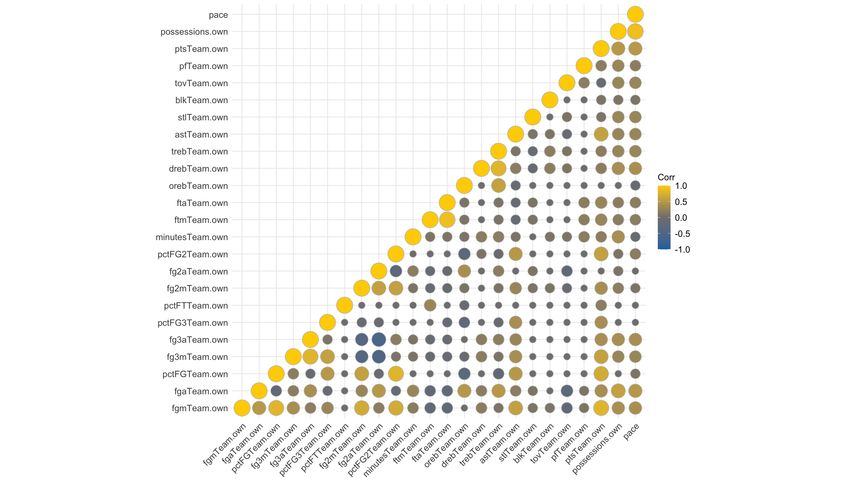
correlations/multicollinearity within the numerical predictors in the dataset. Figure 5.1
shows the breakdown for all correlations between the single-team box score metrics in the
modeling set, including the advanced ones. As one familiar with basketball statistics might
expect, there were some quite highly correlated variables.
Figure 5.1: Correlation matrix for box score statistics.
For example, we calculated pace earlier in the study as basically a per-48 minute trans-
29formation of possessions. And as a result, the correlation between the two variables was 0.9.
Field-goal attempts were highly correlated with field goals made (0.8), free-throw attempts
were associated with free throws made (0.9), and total rebounds were correlated to defensive
rounds (0.8). Additionally, all of the shooting percentage metrics (field-goal percentage, two-
point field-goal percentage, three-point percentage), were highly associated with the shooting
attempts metrics.
Many of the standard NBA box score statistics are interrelated, which is why the analytics
communities have crafted advanced metrics that factor in many of these raws statistics into
a catch-call measure. Examples of these are “true shooting percentage” and “defensive
rebounding percentage”.1 In further studies, it would be prudent to examine these advanced
metrics developed by basketball’s analytics community when building probability models
similar to the one in this study. Regardless, for this research, we will stick to our available
box score metrics and keep in mind the opportunity to eliminate these correlated variables
when choosing the best predictors for the model.
Additionally, before any model building, we must examine if there is any apparent need
for transformations of our box scores metrics. Correlations indicate whether there might be
confounding issues between two different variables, but equally as important to investigate is
if there exists skewness within the distribution of a single variable. Ideally, the distribution
of numerical predictors in our model would resemble a symmetric distribution and normal
curve. Normalized variables perform better in models. The density matrix in Figure 5.2
allows us to examine the distribution of all our numerical predictors.
We see in Figure 5.2 that the variable distributions (even when parsed between wins and
losses) do not show any glaring skewness or multi-modality in our variable set. Recall, at the
end of Chapter 4, we took these raw box score metrics and scaled them to a per-possession
basis. Fortunately, we see the distribution of possessions also appears quite normal, imply-
ing that taking the box score statistics and scaling them by possessions will maintain the
normality. We can conclude that proceeding without any transformations should suffice.
1
https://www.basketball-reference.com/about/glossary.html
30Figure 5.2: Density distribution matrix for box score statistics.
5.1 Logistic Regression
Since our response outcome is a binary variable (team 1 either won or lost) we would be
remiss to not begin the model building process with an attempt at a logistic regression. The
more common, linear regression, is ideal for scenarios where you are predicting an outcome
that has a range of possibilities, usually continuous. For example, how much revenue a
product will generate or how long a flight might take. Whereas with a logistic regression the
predicted Y values are restricted by asymptotes that exist at 0 and 1. Logistic regression is
reserved for models with two outcomes: whether a patient tests positive or negative for a
disease, if a person will default on their credit or not, or if a team will win or lose a matchup.
In fact, for our particular study, logistic regression is a perfect model type to explore as
it does not output a single binary response. Logistic models return a probability score that
31reflects the predicted probability of the occurrence of that event. That probability is then
rounded (usually at 50%) to determine whether the model predicts a positive or negative
response. Figure 5.3 depicts a logistic regression curve and the range of outcomes that can
be outputted from a model. [Jos19]
Figure 5.3: Simplified examples of linear regression versus logistic regression. [Jos19]
Logistic models, and most machine learning algorithms, operate best when only the top
critical features are included. Reasons for this reality of model building are many: fewer
features allow for algorithms to train faster, improves the interpretability of the final result,
reduces overfitting, and, when properly selected, fewer features can improve the accuracy of
a model versus one with far more. We examined two separate methods for feature selection:
recursive feature elimination and stepwise selection.
To conduct the model building in this study we used the caret package in R. Caret
is short for “classification and regression training” and contains a variety of tools to prep
the data for modeling, build training and testing sets, and has over 200 different machine
learning algorithms available. Caret also provided the functionality necessary to perform
feature selection techniques and hyperparameter tuning. All the modeling and evaluation
code can be found on GitHub. [Dot20].
Recursive feature elimination (RFE) finds the best performing feature subset by utilizing
a greedy optimization algorithm. Essentially it repeatedly makes model after model and sets
aside the best features after going through all iterations. In the end, it ranks the variables
32You can also read