A three-dimensional niche comparison of Emiliania huxleyi and Gephyrocapsa oceanica: reconciling observations with projections - Biogeosciences
←
→
Page content transcription
If your browser does not render page correctly, please read the page content below
Biogeosciences, 15, 3541–3560, 2018
https://doi.org/10.5194/bg-15-3541-2018
© Author(s) 2018. This work is distributed under
the Creative Commons Attribution 4.0 License.

A three-dimensional niche comparison of Emiliania huxleyi and
Gephyrocapsa oceanica: reconciling observations with projections
Natasha A. Gafar and Kai G. Schulz
Centre for Coastal Biogeochemistry, School of Environment Science and Engineering,
Southern Cross University, Lismore, NSW 2480, Australia

Correspondence: Natasha A. Gafar (n.gafar.10@student.scu.edu.au)

Received: 14 February 2018 – Discussion started: 1 March 2018
Revised: 21 May 2018 – Accepted: 1 June 2018 – Published: 15 June 2018

Abstract. Coccolithophore responses to changes in carbon-        ticulate inorganic carbon (PIC) with an R 2 of 0.73, p < 0.01
ate chemistry speciation such as CO2 and H+ are highly           and a slope of 1.03 for austral winter/boreal summer and an
modulated by light intensity and temperature. Here, we fit       R 2 of 0.85, p < 0.01 and a slope of 0.32 for austral sum-
an analytical equation, accounting for simultaneous changes      mer/boreal winter.
in carbonate chemistry speciation, light and temperature, to
published and original data for Emiliania huxleyi, and com-
pare the projections with those for Gephyrocapsa ocean-
ica. Based on our analysis, the two most common bloom-           1   Introduction
forming species in present-day coccolithophore communi-
ties appear to be adapted for a similar fundamental light        Since the Industrial Revolution in the late 18th century,
niche but slightly different ones for temperature and CO2 ,      burning of fossil fuels as well as wide-scale deforestation
with E. huxleyi having a tolerance to lower temperatures and     have contributed to significant increases in atmospheric car-
higher CO2 levels than G. oceanica. Based on growth rates,       bon dioxide, CO2 (IPCC, 2013a). Depending upon the deci-
a dominance of E. huxleyi over G. oceanica is projected be-      sions in the next few decades, atmospheric CO2 levels are
low temperatures of 22 ◦ C at current atmospheric CO2 levels.    projected to reach between 420 µatm, which is the Repre-
This is similar to a global surface sediment compilation of      sentative Concentration Pathway (RCP) 2.6 scenario, and
E. huxleyi and G. oceanica coccolith abundances suggesting       985 µatm (RCP8.5 scenario) by 2100 (Caldeira and Wick-
temperature-dependent dominance shifts. For a future Repre-      ett, 2005; Orr et al., 2005; IPCC, 2013a). To date, approxi-
sentative Concentration Pathway (RCP) 8.5 climate change         mately one-third of the anthropogenic carbon emissions have
scenario (1000 µatm f CO2 ), we project a CO2 driven niche       been absorbed by the world’s oceans (Sabine et al., 2004).
contraction for G. oceanica to regions of even higher tem-       As atmospheric partial pressures of CO2 (pCO2 ) increase,
peratures. However, the greater sensitivity of G. oceanica to    CO2 concentrations in the surface ocean also increase, re-
increasing CO2 is partially mitigated by increasing tempera-     sulting in increased bicarbonate and hydrogen ions but also
tures. Finally, we compare satellite-derived particulate inor-   in decreased carbonate ion concentrations and pH (Doney
ganic carbon estimates in the surface ocean with a recently      et al., 2009; Schulz et al., 2009). These changes, often termed
proposed metric for potential coccolithophore success on the     ocean carbonation and acidification, can have both positive
community level, i.e. the temperature-, light- and carbonate-    and negative effects for different phytoplankton species and
chemistry-dependent CaCO3 production potential (CCPP).           groups (e.g. Engel et al., 2005; Feng et al., 2010; Moheimani
Based on E. huxleyi alone, as there was interestingly a better   and Borowitzka, 2011; Endo et al., 2013; Schulz et al., 2017).
correlation than when in combination with G. oceanica, and          Associated with rising pCO2 is the phenomenon of global
excluding the Antarctic province from the analysis, we found     warming. Under current scenarios, ocean temperatures are
a good correlation between CCPP and satellite-derived par-       projected to increase from 2.6 to 4.8 ◦ C by 2100 (IPCC,
                                                                 2013b). In addition, warming of the ocean is expected to en-

Published by Copernicus Publications on behalf of the European Geosciences Union.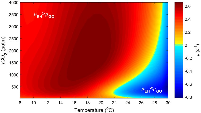
3542                                        N. A. Gafar and K. G. Schulz: Niche comparison of E. huxleyi and G. oceanica

hance vertical stratification of the water column, resulting in   as temperature, light and pCO2 , required for survival of
a shoaling of the surface mixed layer and increasing over-        a species assuming no other species are present (Leibold,
all light and decreasing nutrient availability in the euphotic    1995). However, species do not exist in a vacuum, and where
zone (Bopp et al., 2001; Rost and Riebesell, 2004; Lefeb-         the niche of a species overlaps with another species inter-
vre et al., 2012). While increased light intensity and temper-    actions such as competition for resources and predation can
atures often accelerate growth in phytoplankton, excessive        occur (Hutchinson, 1957; Leibold, 1995), resulting in the re-
levels of light and temperature can cause damage to the pho-      alised niche (Leibold, 1995; Zurell et al., 2016). Hence, it is
tosynthetic apparatus and reduce effectiveness of enzymes,        not only important to determine how environmental change
thus decreasing growth (Powles, 1984; Rhodes et al., 1995;        shapes the fundamental niche of individual species but also
Crafts-Brandner and Salvucci, 2000; Zondervan et al., 2002;       consider the impact of niche overlap of different species in
Helm et al., 2007; Pörtner and Farrell, 2008). Meanwhile,         shaping the realised niches and hence community composi-
reduced nutrient availability could diminish overall produc-      tion.
tivity.                                                              In the present study, we therefore compare species-specific
   Coccolithophores play an important role in the marine car-     sensitivities and responses to combined light, temperature
bon cycle through the precipitation of calcium carbonate, via     and carbonate chemistry changes of two of the most abun-
calcification and the formation and settling of coccolith ag-     dant coccolithophores (Emiliania huxleyi and Gephyrocapsa
gregates, as well as inorganic carbon fixation by photosyn-       oceanica). For that purpose, E. huxleyi was grown at 12
thesis (Rost and Riebesell, 2004; Broecker and Clark, 2009;       pCO2 levels and five light intensities, and growth, photosyn-
Poulton et al., 2007, 2010). The coccolithophores Emilia-         thetic carbon fixation and calcification rates were measured
nia huxleyi and Gephyrocapsa oceanica are considered the          in response. These data were then combined with a previ-
most common species in present-day coccolithophore com-           ously published dataset on temperature and CO2 interaction
munities. E. huxleyi is a ubiquitous coccolithophore hav-         (Sett et al., 2014) and fitted to an analytical equation de-
ing been observed from polar to equatorial regions, from          scribing the combined effects of changing carbonate chem-
nutrient-poor ocean gyres to nutrient-rich upwelling systems      istry speciation, light and temperature. The resulting projec-
and from the bright sea surface down to 200 m depth (McIn-        tions are then compared to those previously published for G.
tyre and Bé, 1967; Winter et al., 1994; Hagino and Okada,         oceanica (Gafar et al., 2018) in an attempt to assess their
2006; Boeckel and Baumann, 2008; Mohan et al., 2008;              individual success and potential realised niche in a chang-
Henderiks et al., 2012). The wide tolerance of E. huxleyi         ing ocean. Finally, we compare satellite-derived particulate
to different environmental conditions is believed to be, at       inorganic carbon estimates with a recently proposed met-
least partially, explained by the existence of several envi-      ric for coccolithophore success on the community level, i.e.
ronmentally selected ecotypes and morphotypes within the          the temperature-, light- and carbonate-chemistry-speciation-
species (Paasche, 2001; Cook et al., 2011). G. oceanica is        dependent calcium carbonate potential (Gafar et al., 2018).
also found in most oceanographic regions (McIntyre and Bé,
1967; Okada and Honjo, 1975; Roth and Coulbourn, 1982;
Knappertsbusch, 1993; Eynaud et al., 1999; Andruleit et al.,      2     Methods
2003; Saavedra-Pellitero et al., 2014), however with a ten-
dency towards warmer waters with very few specimens ob-           2.1    Experimental setup
served below 13 ◦ C (McIntyre and Bé, 1967; Eynaud et al.,
1999; Hagino et al., 2005). It is well established that ris-      To accurately identify optimal conditions, tipping points and
ing pCO2 will have significant effects on coccolithophorid        sensitivities of rates in response to changing CO2 , light and
growth, calcification and photosynthetic carbon fixation rates    temperature, a broad range of experimental conditions are re-
(Riebesell et al., 2000; Bach et al., 2011; Raven and Craw-       quired. Hence, monospecific cultures of the coccolithophore
furd, 2012). Furthermore, it has been shown that the re-          E. huxleyi (strain PML B92/11 morphotype A isolated from
sponse to rising pCO2 of both G. oceanica and E. huxleyi is       Bergen, Norway) were grown in artificial seawater (ASW) at
strongly influenced by light intensity and temperature (Zon-      20 ◦ C and a salinity of 35 across a pCO2 (partial pressure
dervan et al., 2002; Schneider, 2004; De Bodt et al., 2010;       of CO2 ) gradient from ∼ 25 to 7000 µatm. Light intensities
Sett et al., 2014; Zhang et al., 2015). However, to which de-     were set to 50, 400 and 600 µmol photons m−2 s−1 of photo-
gree species-specific responses may shape individual distri-      synthetically active radiation (PAR) on a 16:8 h light–dark
bution and abundance in the future ocean is far less clear.       cycle in a Panasonic versatile environmental test chamber
   This is because the distribution and abundance of a species    (MLR-352-PE). An additional set of cultures was also in-
is controlled by several factors. Firstly, each species has       cubated at 1200 µmol photons m−2 s−1 under a Philips SON-
a specific range of environmental conditions under which          T HPS 600W light in a water bath set to 20 ◦ C. Light inten-
they can successfully grow and reproduce called the fun-          sities at each bottle position for all experiments were mea-
damental niche. The fundamental niche describes the multi-        sured using a LI-193 spherical sensor (LI-COR). Cells were
dimensional combination of environmental conditions, such         pre-acclimated to experimental conditions for 8–12 genera-

Biogeosciences, 15, 3541–3560, 2018                                                   www.biogeosciences.net/15/3541/2018/
N. A. Gafar and K. G. Schulz: Niche comparison of E. huxleyi and G. oceanica                                                3543

tions. To account for differences in growth rate between the      tions to measured final DIC and double the particulate inor-
extreme high/low CO2 treatments and the intermediate CO2          ganic carbon build-up during incubations to measured final
treatments, initial cell densities were chosen between 20 and     TA concentrations. Carbonate chemistry speciation for each
80 cells mL−1 . Treatments were run using a dilute-batch cul-     treatment was calculated from mean TA, mean DIC, mea-
ture setup, mixed daily and harvested before dissolved inor-      sured temperature, salinity and [PO3−
                                                                                                      4 ] using the program
ganic carbon (DIC) consumption exceeded 10 %.                     CO2SYS (Lewis et al., 1998), the dissociation constants for
                                                                  carbonic acid determined by Lueker et al. (2000), KS for sul-
2.2   Media                                                       furic acid determined by Dickson et al. (1990) and KB for
                                                                  boric acid following Uppström (1974).
ASW with a salinity of 35 was prepared according to Kester
et al. (1967). ASW was enriched with f/8 trace metals             2.4   Particulate organic and inorganic carbon
(ethylenediaminetetraacetic acid (EDTA)-bound Fe, Cu, Mo,
Zn, Co, Mn) and vitamins (thiamine, biotin, cyanocobal-           Sampling started approximately 2 h after the onset of the
amin) according to Guillard (1975), 64 µmol kg−1 nitrate          light period and lasted no longer than 3 h. Duplicate sam-
(NO−                −1 phosphate (PO3− ), 10 nmol kg−1 SeO        ples for total and particulate organic carbon (TPC and POC)
     3 ), 4 µmol kg                   4                    2
and 1 mL kg    −1  of coastal seawater (collected at Shelly       were filtered (−200 mbar) onto GF/F filters (Whatmann, pre-
Beach, Ballina, NSW, Australia) to prevent possible limita-       combusted at 500 ◦ C for 4 h) and stored in glass petri dishes
tion by trace elements during culturing which had not been        (precombusted at 500 ◦ C for 4 h) at −20 ◦ C until analysis.
added to the artificial seawater mix. ASW medium was ster-        POC filters were placed in a desiccator above fuming (37 %)
ile filtered (0.2 µm pore size, Whatman™ Polycap 75 AS)           HCl for 2 h to remove all particulate inorganic carbon (PIC).
directly into autoclaved acclimation (0.5 L) or experimen-        All filters were dried overnight at 60 ◦ C and analysed for car-
tal (2 L) polycarbonate bottles (Nalgene® ), leaving a small      bon content and corresponding isotopic signature according
headspace for the adjustment of carbonate chemistry condi-        to Sharp (1974) on an elemental analyser (Flash EA, Thermo
tions.                                                            Fisher) coupled to an isotope ratio mass spectrometer (IRMS,
                                                                  Delta V plus, Thermo Fisher). PIC was calculated by sub-
2.3   Carbonate chemistry manipulation, measurements              tracting measured POC from TPC.
      and calculation
                                                                  2.5   Growth
Carbonate chemistry, i.e. total alkalinity (TA) and DIC, for
                                                                  Cell densities were measured every 3–4 days after the
each treatment was adjusted through calculated additions of
                                                                  commencement of the experiment using a flow cytome-
hydrochloric acid (certified 3.571 mol L−1 HCl, Merck) and
                                                                  ter (Becton Dickinson FACSCalibur) on high flow settings
Na2 CO3 (Sigma-Aldrich, TraceSELECT® quality, dried for
                                                                  (58 µL min−1 ) for 2 min per measurement. Living cells were
2 h at 240 ◦ C). Samples for TA and DIC measurements were
                                                                  detected by their red autofluorescence in relation to their or-
taken at the end of the experiment. TA samples were filtered
                                                                  ange fluorescence in scatter plots (FL3 vs. FL2). At both the
through GF/F filters, stored in the dark at 4 ◦ C and processed
                                                                  extreme low and high CO2 treatments, carbonate chemistry
within 7 days (Dickson et al., 2007; SOP 1). TA samples
                                                                  at the end of the pre-incubation phase can significantly de-
were measured by potentiometric titration using a Metrohm
                                                                  viate from initial and hence experimental treatment condi-
Titrino Plus automatic titrator with 0.05 mol kg−1 HCl as the
                                                                  tions due to enhanced air/water CO2 gas exchange during
titrant, adjusted to an ionic strength of 0.72 mol kg−1 with
                                                                  regular cell abundance monitoring. As a result, at some ex-
NaCl (Dickson et al., 2007; SOP 3b).
                                                                  treme CO2 levels, there was an initial lag phase, and there-
   DIC samples were sterile filtered by gentle pressure filtra-
                                                                  fore growth rates were calculated from densities only during
tion with a peristaltic pump (0.2 µm pore size polycarbonate,
                                                                  the exponential part of the growth phase. After disregarding
Sartorius) into glass stoppered 100 mL bottles (Schott Du-
                                                                  lag-phase measurements, the majority of treatments had only
ran) with overflow of at least 50 % of bottle volume similar
                                                                  two to three data points in the exponential phase. As a result,
to Bockmon and Dickson (2014), sealed without headspace
                                                                  specific growth rates were calculated as
and stored in the dark at 4 ◦ C until processing within 7 days.
To determine DIC, 2 mL of sample was analysed on a Mar-                 ln(Cf ) − ln(C0 )
ianda AIRICA system by acidification with 10 % phosphoric         µ=                      ,                                   (1)
                                                                                d
acid to convert all DIC into CO2 , followed by extraction with
N2 (5.0) and concomitant CO2 analysis with an IR detector         where Cf represents cell densities at time of sampling, C0
(LI-COR LI-7000 CO2 / H2 O analyser). Both TA and DIC             represents cell densities at the beginning of the exponential
measurements were calibrated against certified reference ma-      growth phase, and d is the duration of the exponential phase
terials (batches 139, 141 and 150) following Dickson (2010).      in days. Calcification and photosynthetic rates were calcu-
Initial DIC and TA concentrations were estimated by adding        lated by multiplying cellular PIC and POC quotas with re-
measured total particulate carbon build-up during incuba-         spective growth rates.

www.biogeosciences.net/15/3541/2018/                                                     Biogeosciences, 15, 3541–3560, 2018
3544                                          N. A. Gafar and K. G. Schulz: Niche comparison of E. huxleyi and G. oceanica
                                                                                                              √
2.6    Fitting procedure                                             square root transformed with light (I ) = PFD, where PFD
                                                                     is the photon flux density (µmol photons m−2 s−1 ) of an in-
Coccolithophore metabolic rate (MR) responses of growth,             cubation. To accommodate for known temperature inhibition
calcification and photosynthetic carbon fixation to combined         below 2 and above 30 ◦ C (Rhodes et al., 1995; van Rijssel
changes in temperature, light and carbonate chemistry speci-         and Gieskes, 2002; Helm et al., 2007; Zhang et al., 2014) at
ation can be described as follows (Gafar et al., 2018):              a much narrower experimental range (10–20 ◦ C), the upper
                                                                     and lower limits for E. huxleyi growth were added into the
MR(T , I, S, H )                                                     equation with a general transform of T = (Tt −2)×(30−Tt ),
                            k1 SIT                                   where Tt is the temperature of an incubation. To accurately
=                                                          , (2)     express the onset of high temperature inhibition, the trans-
      k2 HT + k3 SHT + k4 I + k5 SI + SIT + k6 SHI2 T 2
                                                                     form was further modified
                                                                                         √        with a square root transform to
where          k1       (pg       C          cell−1 d−1        or    give T = (Tt −2)× (30 − Tt ). This transform produces rea-
  −1
d ),            k2         (µmol photons m−2 s−1 ),            k3    sonable results when compared to the Eppley temperature en-
(kg mol−1 µmol photons m−2 s−1 ), k4 (mol kg−1 ◦ C), k5              velope curve and the Norberg model (see Gafar et al., 2018).
(◦ C), k6 (kg mol−1 µmol photons−1 m2 s ◦ C−1 ) are fit coeffi-
cients, and MR (T , I , S, H ) is the metabolic rate of photo-       2.8   Physiological rate response parameter estimations
synthesis, calcification or growth dependent on temperature                to changes in carbonate chemistry, temperature
(T ), light intensity (I ), substrate (S = [CO2 ] + [HCO−                  and light
                                                              3 ])
and [H+ ] (H ). Inputs to the equation consisted of calculated
CO2 , HCO−             + (H in total scale) concentrations,          Equation (2) was used to assess the combined effects of car-
             3 and H
as well as measured metabolic rates, and light (I ) and              bonate chemistry, temperature and light on growth, calcifi-
temperature (T ) levels of all treatments (please see below          cation and photosynthetic carbon fixation rates, with a focus
for information on temperature and light transforms).                on general physiological features, such as limitation and in-
   Data from this study (Tables S1, S2) and Sett et al. (2014)       hibition, as well as how much variability could be explained.
were fitted to Eq. (2) using the non-linear regression fit pro-      For growth, photosynthetic carbon fixation and calcification
cedure nlinfit in MATLAB (MathWorks). The reason only                rates of optimum CO2 concentrations for maximum produc-
these studies were chosen, from the multitude of E. hux-             tion rates (Vmax ) and half-saturation values were calculated
leyi datasets, is because (1) they use the same strain (PML          at each experimental light and temperature level. K 12 values
B92/11), (2) they have the same nutrient conditions, and             consisted of K 12 CO sat which is the CO2 concentration (at
                                                                                           2
(3) they use the same carbonate chemistry manipulation               certain T and I) at which rates are saturated to half the max-
methods. Nevertheless, the two chosen studies provided light         imum, and K 21 CO inhib, which is the CO2 concentration (at
                                                                                         2
(six levels) and temperature (three levels) interactions over a      certain T and I ) at which high proton concentrations reduce
broad carbonate chemistry speciation range. It is noted that         physiological rates to half the maximum. Fitting results (R 2 ,
in both studies the carbonate chemistry system is coupled,           fit coefficients, p values, F values and degrees of freedom),
meaning that a change in CO2 results in a change in pH. This         as well as Vmax , K 12 and CO2 optima are presented in Ta-
method reflects the changes in carbonate chemistry specia-           bles 1, 2 and 3. Species-specific differences in response to
tion due to ongoing ocean acidification (Bach et al., 2011,          changing carbonate chemistry, temperature and light were as-
2013). However, some studies have examined the effects of            sessed by comparing the above fit to that recently produced
decoupled carbonate chemistry where CO2 is changed at a              for Gephyrocapsa oceanica (Gafar et al., 2018).
constant pH. This approach is used to tease apart the inde-
pendent effects of H+ and CO2 on physiological responses             2.9   Niche comparison
(see Bach et al., 2013). While Eq. (2) can also be used to ex-
plain responses under decoupled carbonate chemistry condi-           To examine the potential of ongoing ocean change to influ-
tions (see Gafar et al., 2018 for details), the fit obtained here    ence realised niches, and hence individual success, ranges
is only valid for coupled CO2 /pH changes as no data from de-        for light and temperature where both Emiliania huxleyi and
coupled experiments (i.e. Bach et al., 2011) have been used.         Gephyrocapsa oceanica might be expected to coexist were
The reason for this is that Bach et al. (2011) does not contain      selected (i.e. 50–1000 µmol photons m−2 s−1 and 8–30 ◦ C).
data of temperature, light and carbonate chemistry interac-          E. huxleyi and G. oceanica were chosen for comparison as
tions.                                                               they are currently the only two species with response data
                                                                     over a range of carbonate chemistry, temperature and light
2.7    Temperature and light transformations                         conditions. Growth rates were selected as the point of com-
                                                                     parison because they can be used as a measure of relative
To reduce skew and to better accommodate certain features            abundance and therefore dominance of a species, and be-
(i.e. light and temperature inhibition and limitation), both         cause growth rates largely control carbon fixation rates. To
temperature and light data were transformed. Light data were         assess competitive ability, and the potential realised niche,

Biogeosciences, 15, 3541–3560, 2018                                                      www.biogeosciences.net/15/3541/2018/
N. A. Gafar and K. G. Schulz: Niche comparison of E. huxleyi and G. oceanica                                                                  3545

Table 1. Fit coefficients (k1 to k6 ), R 2 , F values, degrees of freedom and p values obtained for calcification (pg C cell−1 d−1 ), photosynthetic
carbon fixation (pg C cell−1 d−1 ) and growth rates (d−1 ) from Eq. (2) fitted to data from this study and Sett et al. (2014). For calcification
and photosynthetic carbon fixation rates, the unit for v is pg C cell−1 d−1 , while for growth rates, the unit for v is d−1 .

                                                                       Calcification      Photosynthesis               Growth
                    k1 (pg C cell−1 d−1 or d−1 )                            −11.98                −17.68                −0.71
                    k2 (µmol photons m−2 s−1 )                         −1.75 × 10⁶           −4.63 × 10⁶          −9.34 × 10⁵
                    k3 (kg mol−1 µmol photons m−2 s−1 )                 6.43 × 10⁷            1.39 × 10⁹           3.10 × 10⁸
                    k4 (mol kg−1 ◦ C)                                        −0.22                 −0.23        −7.28 × 10⁻²
                    k5 (◦ C)                                                  28.14                 26.72              −38.72
                    k6 (kg mol−1 µmol photons−1 m2 s ◦ C−1 )           −3.09 × 10³            4.40 × 10³          −2.70 × 10³
                    R 2 (p value)                                  0.7957 (< 0.001)      0.7302 (< 0.001)     0.8460 (< 0.001)
                    F value (degrees of freedom)                      389.51 (100)          273.52 (100)         552.74 (100)

Table 2. Optimum CO2 concentrations, CO2 K 12 concentrations and maximum rates (Vmax ) at 10, 15 and 20 ◦ C from Eq. (2) fit to CO2
light data at 20 ◦ C in this paper, and E. huxleyi CO2 data from Sett et al. (2014) at 10, 15 and 20 ◦ C and 150 µmol photons m−2 s−1 light
intensity. Note that the CO2 working range for the equation for this species was 0–250 µmol kg−1 . Values exceeding this range were reported
as > 250 µmol kg−1 .

                                       CO2                                      10 ◦ C     15 ◦ C    20 ◦ C
                                       CO2 optima (µmol kg−1 )
                                       Calcification                            16.94      12.91      11.50
                                       Photosynthesis                           20.34      15.42      13.91
                                       Growth rate                              29.06      20.78      18.36
                                       Vmax
                                       Calcification (pg C cell−1 d−1 )          6.37       8.94       9.69
                                       Photosynthesis (pg C cell−1 d−1 )         8.55      11.52      12.22
                                       Growth rate (d−1 )                        0.59       1.08       1.38

                                       K 21 CO inhib (µmol kg−1 )
                                              2
                                       Calcification                           118.47     75.04      62.94
                                       Photosynthesis                           > 250    119.54     100.51
                                       Growth rate                              > 250     > 250     192.74

                                       K 21 CO sat (µmol kg−1 )
                                              2
                                       Calcification                             1.66       1.56       1.48
                                       Photosynthesis                            1.65       1.50       1.42
                                       Growth rate                               0.85       1.19       1.40

the difference in growth rates between the species was visu-                be a suitable proxy for species dominance. It is noted that
alised using contour plots.                                                 E. huxleyi has been found to produce excess coccoliths to-
   The effect of temperature on growth rates and hence po-                  wards the end of blooms when inorganic nutrients become
tential dominance was then compared to phytoplankton com-                   limiting for cellular growth (Balch et al., 1992; Holligan
munity data from global surface sediment samples above the                  et al., 1993; Paasche, 1998), which would result in an over-
lysocline (McIntyre and Bé, 1967; Chen and Shieh, 1982;                     estimate of E. huxleyi dominance in our study. Nevertheless,
Roth and Coulbourn, 1982; Knappertsbusch, 1993; Andruleit                   given that the coccoliths’ ratio varies orders of magnitude in
and Rogalla, 2002; Boeckel et al., 2006; Fernando et al.,                   modern marine sediments, none of our general conclusions
2007; Saavedra-Pellitero et al., 2014). As E. huxleyi and                   should be affected. Temperature for each sampling site was
G. oceanica have similar average numbers of coccoliths                      retrieved from the National Oceanic and Atmospheric Ad-
per cells, 28 and 21, respectively (Samtleben and Schroder,                 ministration (NOAA) 1◦ resolution annual temperature cli-
1992; Knappertsbusch, 1993; Baumann et al., 2000; Boeckel                   matology (Boyer et al., 2013).
and Baumann, 2008; Patil et al., 2014), the abundance ratio
of E. huxleyi to G. oceanica coccoliths was here assumed to

www.biogeosciences.net/15/3541/2018/                                                                   Biogeosciences, 15, 3541–3560, 2018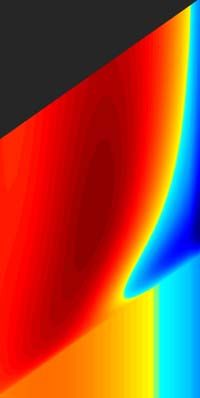
3546                                             N. A. Gafar and K. G. Schulz: Niche comparison of E. huxleyi and G. oceanica

Table 3. Optimum CO2 concentrations, CO2 K 12 concentrations and maximum rates (Vmax ) at 50–1200 µmol photons m−2 s−1 from Eq. (2)
fit to CO2 data at 50, 400, 600 and 1200 µmol photons m−2 s−1 and 20 ◦ C in this paper and E. huxleyi CO2 data from Sett et al. (2014)
at 150 µmol photons m−2 s−1 light intensity and 10, 15 and 20 ◦ C. Note that the CO2 working range for the equation for this species was
0–250 µmol kg−1 . Values exceeding this range were reported as > 250 µmol kg−1 .

                      CO2                                  50 PAR   150 PAR     400 PAR     600 PAR     1200 PAR
                      CO2 optima (µmol kg−1 )
                      Calcification                          8.39      11.67       15.21       16.75        19.14
                      Photosynthesis                         9.92      14.47       21.44       26.47        52.12
                      Growth rate                           14.97       19.1       21.26       21.32        20.23
                      Vmax
                      Calcification (pg C cell−1 d−1 )       7.64      10.05       12.47       13.48        15.04
                      Photosynthesis (pg C cell−1 d−1 )      9.16      12.78       17.27       19.82        27.24
                      Growth rate (d−1 )                     1.19       1.43        1.58        1.61         1.62

                      K 12 CO inhib (µmol kg−1 )
                             2
                      Calcification                         47.38      63.01       80.19       87.68        99.10
                      Photosynthesis                        73.04     104.90      182.32       > 250        > 250
                      Growth rate                          157.71     208.62      206.04      192.60       163.64

                      K 12 CO sat (µmol kg−1 )
                             2
                      Calcification                          1.00       1.53        2.13        2.39         2.81
                      Photosynthesis                         0.90       1.49        2.38        2.96         4.99
                      Growth rate                            1.08       1.46        1.69        1.73         1.72

2.10   Global calcium carbonate production potential                  a week by a coccolithophore community (with a set start-
                                                                      ing cell count) for a certain environmental condition, calcu-
While our fit equation has previously explained variability in        lated from Eq. (2) derived growth rates and inorganic carbon
lab experiments quite well (Gafar et al., 2018), natural sys-         quotas. Inorganic carbon quotas are calculated as the quo-
tems are much more complex, with the interactions of dozens           tient of calcification and growth rates. As CCPP is calculated
of variables including temperature, light, nutrients, predation       from calcification and growth rates, it accounts for the indi-
and competition all influencing productivity (Behrenfeld,             vidual effects of temperature, light and carbonate chemistry
2014). As such, we wanted to examine how projections of               on growth rates and on carbon production. It was for these
productivity using our relatively simple equation compared            reasons that CCPP was the metric chosen for comparison.
to coccolithophorid productivity patterns observed in natural            Provided values for temperature, light, substrate
systems. Productivity can be defined in a few ways; tradi-            (CO2 + HCO−     3 ) and hydrogen ion concentrations (H)
tionally, changes in cellular calcification rates, in response        for the surface mixed layer, coccolithophore CaCO3 produc-
to ocean change, have been used as indicator for the poten-           tion potential can be projected for the world oceans. CCPP
tial success of coccolithophores in the future ocean. How-            can then be cautiously evaluated against and compared
ever, the exponential nature of phytoplankton growth ampli-           to satellite-derived global particulate inorganic carbon
fies even small differences in cellular growth rates, when ap-        concentration estimates (PICs ). As inorganic nutrients are
plied on the community level. For instance, a phytoplankton           a critical factor influencing phytoplankton abundance, and
bloom occurring over 1 week at a growth rate of 1.0 d−1 and           especially bloom formation, in the ocean (Browning et al.,
a starting cell density of 50 cells mL−1 would lead to a peak         2017), nitrate concentrations were also included in the
density of about 55 000 cells mL−1 . This is in stark contrast        analysis (for details, see below). As a result, climatological
to conditions where growth is only 10 % lower as peak cell            datasets consisted of World Ocean Atlas (WOA) 2013
densities, and hence biomass and PIC standing stock, will             v2 nitrate concentrations at 1◦ resolution (Boyer et al.,
only be half.                                                         2013); SeaWiFS mixed layer depth (MLD 2◦ resolution)
   Recently, a new metric was proposed, the CaCO3 produc-             from de Boyer Montégut et al. (2004); surface photosyn-
tion potential (CCPP), which (1) should be a better represen-         thetically available radiation (PAR µmol photons m−2 s−1
tation of potential coccolithophore success on the commu-             9 km resolution) from the Moderate Resolution Imaging
nity level and (2) can be tested against modern observations          Spectroradiometer (MODIS)-Aqua (NASA Goddard Space
of surface ocean CaCO3 distribution (Gafar et al., 2018).             Flight Center, 2014b); diffuse attenuation coefficients at
CCPP is defined as the amount of CaCO3 produced within                490 nm (9 km resolution) from Pascal (2013); and NOAA

Biogeosciences, 15, 3541–3560, 2018                                                         www.biogeosciences.net/15/3541/2018/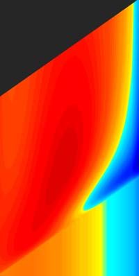
N. A. Gafar and K. G. Schulz: Niche comparison of E. huxleyi and G. oceanica                                                3547

dissolved inorganic carbon, pCO2 , pH (total scale), [CO2−
                                                        3 ],       0.25 mL−1 for G. oceanica alone and 0.25 mL−1 for each
temperature and salinity (4 × 5◦ resolution) from Takahashi        species when combined. To allow comparison, CCPP and
et al. (2014). A 9 km resolution climatology for particulate       PICs were both converted to units of µmol PIC L−1 . All
inorganic carbon (PICs ) concentration (mol PIC m−3 ) was          data were then averaged for austral summer/boreal win-
also retrieved from MODIS-Aqua (NASA Goddard Space                 ter (December–February) and austral winter/boreal summer
Flight Center, 2014a). Once acquired, all datasets were            (June–August). Austral summer/boreal winter and austral
interpolated to a 1◦ resolution.                                   winter/boreal summer were chosen as they provide promi-
   Hydrogen ion concentrations were calculated as 10−pH ,          nent differences between minimum and maximum PIC,
CO2 , after conversion of pCO2 to f CO2 as described in            while spring and autumn do not. A direct comparison be-
CO2SYS (Lewis et al., 1998), as [f CO2 ] × K0 (with K0             tween PICs and CCPP was achieved by splitting results
being the temperature- and salinity-dependent
                                               Henry’scon-       into major ocean biogeographical provinces following Gregg
                                            2−                     and Casey (2007) with the single change of adjusting the
stant), HCO−        −
           3 as [HCO3 ] = DIC − [CO2 ] + [CO3 ] and                Antarctic and the north ocean regions to start at 45◦ as in
substrate (S) as the sum of CO2 and HCO−                           Longhurst (2007) rather than 40◦ (see Sect. 4.5). For each
                                          3 concentrations.
Mean mixed layer nitrate concentrations were calculated by         major province, the total amount of PICs and CCPP for
determining concentrations for each depth and averaging            all comparable grid cells was calculated for austral sum-
from the surface to the mixed layer depth for each grid cell.      mer/boreal winter and austral winter/boreal summer. For
Mean mixed layer irradiance was calculated in 1 m depth in-        comparison, values for each basin and season were then con-
crements for each grid cell as                                     verted into percentages of annual global (global summer plus
                                                                   global winter) PICs or CCPP production. Agreement be-
     MLD
     X                                                             tween the satellite and CCPP estimates was then assessed
I=         = exp−kd (i) × I0 ,                              (3)
                                                                   using a linear correlation. While three CCPP scenarios are
     i=1
                                                                   presented above, only the results with the highest correlation
where I is the average PAR (µmol photons m−2 s−1 ), kd is the      to satellite PIC are shown and discussed below.
attenuation coefficient (m−1 ), MLD denotes the mixed layer
depth in metres, and I0 is the incident PAR at the surface
(µmol photons m−2 s−1 ).                                           3     Results
   Global coverage of oceanic nutrient concentrations is of-
ten limited to only a few macronutrients (nitrate, silicate,       The fit equation (Eq. 2) was able to explain up to
phosphate). However, concentrations of these nutrients are         85 % of growth, 80 % of calcification and 73 % of pho-
often strongly correlated (e.g. phosphate and nitrate in Boyer     tosynthetic rate variability in E. huxleyi across a broad
et al., 2013). To ensure there were sufficient nutrients to sup-   range of carbonate chemistry (25–4000 µatm), light (50–
port the level of production estimated by CCPP, we opted to        1200 µmol photons m−2 s−1 ) and temperature (10–20 ◦ C)
use a single nutrient, i.e. nitrate, in combination with a sim-    conditions (Table 1).
ple scaling metric. We first assumed a Redfieldian ratio of
106 : 16 C : N to determine the maximum POC production             3.1    E. huxleyi responses to changing carbonate
possible from the amount of available nitrate. We then calcu-             chemistry: CO2 and H+
lated the amount of PIC which would be co-produced based
                                                                   Based on fits of Eq. (2), growth, calcification and photosyn-
on a mean PIC : POC. The average PIC : POC of E. huxleyi
                                                                   thetic carbon fixation rates all had a similar optimum curve
and G. oceanica was calculated as the average of all treat-
                                                                   response to the broad changes in carbonate chemistry spe-
ments between 300 and 1000 µatm from Sett et al. (2014),
                                                                   ciation (Fig. 1) regardless of temperature and light intensi-
Zhang et al. (2015) and this study. Based on these averages
                                                                   ties. Growth, calcification and photosynthetic carbon fixa-
(PIC : POC of 0.8 and 1.35 for E. huxleyi and G. oceanica,
                                                                   tion rates required similar CO2 concentrations, with differ-
respectively), and assuming Redfieldian production, a corre-
                                                                   ences of less than 3 µmol kg−1 under comparable tempera-
sponding PIC : PON of 5.3 and 8.94 was calculated. Hence,
                                                                   ture and light conditions, to stimulate rates to half the maxi-
maximum CaCO3 production potential (CCPPmax ) in a grid
                                                                   mum, K 12 CO sat (Tables 2, 3). Optimum CO2 concentrations
cell would be 5.3 and 8.94 times the nitrate concentration for                  2

E. huxleyi and G. oceanica, respectively. If estimated CCPP        for calcification (8.4–19.1 µmol kg−1 ) were slightly lower
for a cell exceeded CCPPmax , and therefore the nitrate re-        than for photosynthesis (9.9–52.1 µmol kg−1 ) or growth (15–
quired to produce that much PIC, then it was replaced with         29.1 µmol kg−1 Tables 2, 3). At CO2 concentrations be-
the CCPPmax value. If CCPP was less than Cmax , then no            yond the optimum, a much higher sensitivity to increas-
further changes were applied.                                      ing [H+ ], i.e. K 21 CO inhib, was observed for calcifica-
                                                                                           2
   To ensure that mean global CCPP and mean global PICs            tion (47.4–118.5 µmol kg−1 ) than for photosynthesis (73.0–
would be of the same magnitude, starting cell counts for           250 µmol kg−1 ) or growth rates (157.7–250 µmol kg−1 ; Ta-
CCPP calculations were set at 1 mL−1 for E. huxleyi alone,         bles 2, 3 and Figs. 1, 2).

www.biogeosciences.net/15/3541/2018/                                                      Biogeosciences, 15, 3541–3560, 2018
3548 N. A. Gafar and K. G. Schulz: Niche comparison of E. huxleyi and G. oceanica
15 20
(a) 50 PAR (a)
150 PAR
(pg C cell-1 d-1 )
PIC production
(pg C cell-1 d-1 )
PIC production
15 400 PAR
10 600 PAR
10 1200 PAR
5 5
0
0 0 50 100 150
0 50 100 150 200 250 (b)
15
(b) 30
POC production
(pg C cell-1 d-1 )
POC production
(pg C cell-1 d-1 )
10 20
10
5
0
0 50 100 150
0 2
0 50 100 150 200 250 (c)
2
(c) 1.5
μ (d -1 )
1.5
1
μ (d -1 )
1
0.5
0.5 0
0 50 100 150
-1
0 CO2 (μmol kg )
0 50 100 150 200 250
CO2 (μmol kg-1 ) Figure 2. Fitted (solid lines) and measured (symbols) (a) PIC and
(b) POC production and (c) growth rates of E. huxleyi in response to
Figure 1. (a) Fitted PIC, (b) POC production and (c) growth rates changes in CO2 concentration at six different light intensities using
(solid lines) of E. huxleyi in response to changes in carbonate chem- Eq. (2) and fit coefficients from Table 1. Symbols represent rate
istry at 10, 15 and 20 ◦ C using Eq. (2) and fit coefficients from Ta- measurements from this paper at a constant temperature (20 ◦ C) and
ble 1. Symbols represent rate measurements from Sett et al. (2014) 50, 150, 400, 600 and 1200 µmol photons m−2 s−1 . Shaded areas
at 10, 15 and 20 ◦ C and 150 µmol photons m−2 s−1 . Shaded areas represent modern ocean CO2 concentrations of 8.5–30 µmol kg−1
represent modern ocean CO2 concentrations of 8.5–30 µmol kg−1 based on data from Takahashi et al. (2014).
based on data from Takahashi et al. (2014).
3.3 E. huxleyi responses to light
3.2 E. huxleyi responses to temperature Light intensities affected all physiological rates, with the
greatest effect generally being observed at CO2 concen-
trations at or above the optimum (Fig. 2). Between 50
The effect of temperature on rates was dependent upon CO2 , and 1200 µmol photons m−2 s−1 , calcification rates doubled,
with the greatest effect observed at optimum CO2 concen- photosynthetic rates tripled and growth rates increased
trations (Fig. 1). Increasing temperature increased maximum around 36 % (Fig. 2, Table 3). Both optimum CO2 and CO2
growth rates (Vmax ) up to 2-fold, photosynthetic rates up to concentrations at which rates were half saturated (K 12 CO
2
43 % and calcification rates up to 52 % (Fig. 1, Table 2) un- sat) increased slightly with increasing light intensity (Ta-
der optimal CO2 concentrations. CO2 half-saturation con- ble 3). CO2 concentrations required to inhibit rates to half of
centrations (K 12 CO sat) were insensitive to temperature (Ta- the maximum (K 12 CO inhib) for calcification and photosyn-
2 2
ble 2). However, under increasing temperatures, CO2 con- thesis increased with increasing light intensity, while those
centrations for both optimal growth and for inhibition of rates for growth increased from 50 to 150 µmol photons m−2 s−1
to half the maximum (K 12 CO inhib) decreased (Table 2). before decreasing with further increases in light (Table 3).
2
Biogeosciences, 15, 3541–3560, 2018 www.biogeosciences.net/15/3541/2018/N. A. Gafar and K. G. Schulz: Niche comparison of E. huxleyi and G. oceanica 3549
4 Discussion H+ (Ca2+ + HCO− 3 CaCO3 + H+ ), potentially decreas-
2−
ing [CO3 ] in the coccolith-producing vesicle and hence
4.1 Responses to changing carbonate chemistry: CO2 the CaCO3 saturation state (Bach et al., 2015). Further-
and H+ more, increased [H+ ] has been found to result in declines in
[HCO− 3 ] uptake, the primary carbon source for calcification
Rates of photosynthesis, calcification and growth in coc- (Kottmeier et al., 2016).
colithophores are strongly influenced by CO2 (Bach et al.,
2011; Sett et al., 2014; Zhang et al., 2015). Increasing CO2 4.2 Responses to temperature
concentrations resulted in enhanced rates up to an optimum
level beyond which they then declined again. This pattern in Temperature was observed to have few modulating effects
growth, photosynthetic carbon fixation and calcification rates on CO2 responses in E. huxleyi. Changes in temperature pro-
has been observed previously for several coccolithophore duced little (< 1 µmol kg−1 ) change in CO2 substrate half-
species (Sett et al., 2014; Bach et al., 2015). The availability saturation (K 12 CO sat) levels, at least within the measured
2
of substrate (CO2 and HCO− range (Fig. 1, Table 2). CO2 requirements for optimum rates
3 ) was suggested as the factor
influencing the increase in rates on the left side of the opti- tended to slightly decrease with warming temperatures. Simi-
mum, while the proton concentration ([H+ ]) was the factor lar results were observed for G. oceanica (Gafar et al., 2018).
most likely driving declines to the right side of the optimum This indicates that while overall rates change, carbon uptake
(Bach et al., 2011, 2015). mechanisms appear to scale to maintain internal substrate
Of the two species, E. huxleyi has a higher CO2 optimum concentrations and thus cellular requirements regardless of
than G. oceanica (Tables 2, 3 and S3; Gafar et al., 2018) for temperature conditions.
all rates and under most conditions. This could suggest that In contrast, the inhibition of rates by rising [H+ ], i.e.
1
E. huxleyi has a slightly higher substrate requirement than G. K 2 CO inhib, was more sensitive to temperature. The CO2
2
oceanica. However, considering that G. oceanica has both a concentration at which rates were reduced to half the max-
larger cell size and higher carbon quotas per cell, the oppo- imum increased with decreasing temperatures (Table 2).
site would be expected (Sett et al., 2014; Bach et al., 2015). These results were also observed for G. oceanica which had a
An explanation for achieving maximum rates only at higher lower sensitivity to increasing [H+ ] at the lowest tested tem-
CO2 concentrations in E. huxleyi, in comparison to G. ocean- perature (Gafar et al., 2018). This also agrees with De Bodt
ica despite a lower inorganic carbon demand, might be a less et al. (2010) in which a greater decline in calcification rate
efficient or capable carbon uptake/concentrating mechanism. was observed with increasing CO2 at 18 ◦ C than at 13 ◦ C.
Alternatively, a decreased sensitivity to high [H+ ] in E. hux- These results indicate that at least some coccolithophores
leyi, in comparison to G. oceanica (see below), would lead to may be less sensitive to high CO2 levels at lower tempera-
a shift in the optimum towards higher CO2 as well and might tures. As a result, both G. oceanica and E. huxleyi may be-
be a more likely explanation. come more vulnerable to the negative effects of ocean acidifi-
Of the three rates, calcification in E. huxleyi had both the cation as ocean temperatures increase due to climate change.
lowest CO2 requirement and the highest sensitivity to in-
creasing [H+ ] (Tables 3 and 2). This is a pattern previously 4.3 Responses to light
observed for G. oceanica under varying temperature and
The sensitivity of all rates in E. huxleyi to changing car-
light conditions (Gafar et al., 2018; see also Table S3 in the
bonate chemistry, in particular increasing [H+ ], was clearly
Supplement). As evidenced by higher K 12 CO inhib values
2 modulated by light intensity (Fig. 2), agreeing with earlier
for all processes, E. huxleyi also appears less sensitive to the
findings (Zondervan et al., 2002; Feng et al., 2008; Gao
inhibiting effects of increasing [H+ ] than G. oceanica (i.e.
et al., 2009; Rokitta and Rost, 2012; Zhang et al., 2015).
K 12 CO inhib is 47–250 µmol kg−1 versus 25–99 µmol kg−1
2 CO2 half saturation (K 21 CO sat) for all rates was insensitive
for G. oceanica depending on light intensities or K 21 CO 2
to increasing light intensities (Table S3). This agrees with
2
inhib is 62–250 µmol kg−1 versus 25–130 µmol kg−1 for G. results for G. oceanica which also displayed little change
oceanica depending on temperature) (Tables 2, 3, S3; Ga- in CO2 half-saturation concentrations with increasing light
far et al., 2018). This also supports earlier results in a model (Table S3). Increasing light intensity induced increases in
analysis by Bach et al. (2015) where E. huxleyi reacted less CO2 optima in all rates; however, these changes were small
sensitively to higher CO2 (and [H+ ]) than G. oceanica. (< 10 µmol kg−1 ) for calcification and growth rates. This con-
A lower sensitivity of rates to changes in carbonate chem- trasts with G. oceanica for which a distinct decrease in
istry speciation, in particular calcification rates, could be ex- optimal CO2 concentrations for growth rates with increas-
plained by the lower degree of calcification in E. huxleyi ing light intensities was observed (Table S3). However, G.
(PIC : POC ratios 0.24–1.38) when compared to G. oceanica oceanica projections are based on a dataset with only three
(PIC : POC ratios 0.84–2.44) (Sett et al., 2014). Higher rates CO2 concentrations (∼ 16, 31, 45 µmol kg−1 ). As such, it is
of calcification result in greater production of intracellular difficult to determine how robust the estimates of CO2 op-
www.biogeosciences.net/15/3541/2018/ Biogeosciences, 15, 3541–3560, 20183550 N. A. Gafar and K. G. Schulz: Niche comparison of E. huxleyi and G. oceanica
tima and half-saturation requirements may be for this species 4.4.1 Fundamental niche
(Zhang et al., 2015).
In E. huxleyi, the relationship between H+ sensitivity and Experimentally, E. huxleyi has been found to grow in a range
light intensity was the same for the three rates. Calcification of ∼ 6 to 2500 µmol photons m−2 s−1 with high light result-
and photosynthetic carbon fixation and growth rates were ing in no inhibition of maximum rates in some strains and
most sensitive to H+ at the lowest (50 µmol photons m−2 s−1 ) up to 20 % reduction in others (Balch et al., 1992; van Blei-
and growth rates were also slightly more sensitive at the jswijk et al., 1994; Nielsen, 1995; Nanninga and Tyrrell,
highest (1200 µmol photons m−2 s−1 ) light intensities (Ta- 1996; van Rijssel and Gieskes, 2002). In contrast, G. ocean-
ble 3). This result is in part due to an underestimation of ica is more sensitive in a similar experimental range of ∼ 6–
growth rates by the fitting equation under high CO2 con- 2400 µmol photons m−2 s−1 with maximum rates inhibited
ditions at 50 µmol photons m−2 s−1 light (Fig. 2). However, by up to 38 % at high light intensities (Larsen, 2012). Light
it may be that sub-optimal light intensities add additional intensities below 6 µmol photons m−2 s−1 for E. huxleyi and
stress to the cells resulting in them having less resources with G. oceanica resulted in no growth for both species (van Blei-
which to handle the stress of increasing high [H+ ]. Hence, jswijk et al., 1994; van Rijssel and Gieskes, 2002; Larsen,
rates are lower but also appear more sensitive to changing 2012). So, while G. oceanica is more sensitive to high light,
carbonate chemistry. These findings agree with findings by the potential upper light limit for growth in both species is
Rokitta and Rost (2012) where a diploid E. huxleyi strain beyond naturally occurring maxima. Within this light range,
became insensitive to the effects of rising CO2 (380 vs. both species show a similar increase in projected absolute
1000 µatm) when light intensities were increased from 50 growth rates of 0–1.57 (d−1 ) for E. huxleyi and 0–1.51 (d−1 )
to 300 µmol photons m−2 s−1 . However, this differs from G. for G. oceanica (based on Fig. 4).
oceanica which, with rising light intensities, had no change E. huxleyi has been successfully cultured at pCO2 levels
in sensitivity for calcification rates, a decrease in sensitivity between ∼ 20 and 5600 µatm, while G. oceanica has been
for photosynthesis and an increase in sensitivity for growth successfully cultured at pCO2 levels of ∼ 20–3400 µatm
rates (Table S3). Again, although this could be indicative of (Sett et al., 2014). Again, the upper tolerance limit for growth
species-specific differences in sensitivity, it may also be a re- in both is not known and well above what is expected for
sult of the low number of CO2 treatments used in the light most ocean systems. Responses in projected growth rates
data of G. oceanica (see Zhang et al., 2015). with rising CO2 differ between the two species, with G.
oceanica rates dropping to 50 % of maximum at f CO2 levels
4.4 E. huxleyi and G. oceanica a niche comparison above ∼ 1760 µatm while E. huxleyi drops to 50 % of max-
imum at ∼ 5950 µatm. In terms of temperature, E. huxleyi
In the future ocean CO2 , temperature and light availability has a broader niche of 3–29 ◦ C in comparison to G. ocean-
are all expected to change (Rost and Riebesell, 2004; IPCC, ica at 10–32 ◦ C. Within this temperature niche, both species
2013b). Levels of f CO2 are expected to reach as high as again show a similar change in absolute growth rates of 0–
985 µatm by the end of the century with concomitant rise in 1.40 (d−1 ) for G. oceanica and 0–1.43 (d−1 ) for E. huxleyi
global ocean temperature of up to 4.8 ◦ C (RCP8.5 scenario, (based on Fig. 5).
IPCC, 2013a, b). Light intensities in the surface ocean are It should be noted, however, that although niche ranges
also expected to increase as a result of mixed layer depth and maximum rates are similar for both species, different re-
shoaling (Rost and Riebesell, 2004). By calculating and com- quirements (K 12 sat) and sensitivities K 12 inhib) will lead
paring growth rates for E. huxleyi and G. oceanica over a to different actual rates at a specific environmental condi-
range of environmental conditions, it is possible to differ- tion. This becomes evident when examining the temperature,
entiate between the fundamental (physiological) niche of a light and CO2 niches to find a combination of conditions at
species and its potentially realised niche when in competi- which the growth rate for each species is at its maximum.
tion with others. For this purpose, light, temperature and CO2 For E. huxleyi, maximum growth rates of 1.62 (d−1 ) are
ranges were restricted to those where both species would be projected at ∼ 970 µmol photons m−2 s−1 light, ∼ 640 µatm
expected to co-occur, i.e. 20–1000 µmol photons m−2 s−1 , 8– CO2 and 20.2 ◦ C. In contrast, the conditions for optimal
30 ◦ C and 25–4000 µatm, respectively. The calculated differ- growth rates of 1.52 (d−1 ) for G. oceanica are achieved
ence in growth rates in response to CO2 and temperature does at ∼ 500 µmol photons m−2 s−1 light, ∼ 430 µatm CO2 and
not significantly change with light intensity (Figs. 3 and 4). It 24.4 ◦ C. Differences in sensitivity and therefore performance
should be noted, however, that light intensity might modify under certain conditions will influence the potentially re-
observed growth rate differences for other strains of the same alised niche of the species. For example, E. huxleyi is pro-
species than used here as they can possess different sensitiv- jected to reach higher growth rates than G. oceanica under
ities and requirements (i.e. Langer et al., 2009; Müller et al., a broader range of temperature, light and CO2 conditions
2015). (Figs. 3, 4 and 5), supporting the notion that E. huxleyi is
rather a generalist.
Biogeosciences, 15, 3541–3560, 2018 www.biogeosciences.net/15/3541/2018/N. A. Gafar and K. G. Schulz: Niche comparison of E. huxleyi and G. oceanica 3551
0.6
4000 0.4
0.2
3000
fCO2 (μatm)
μ (d-1)
0
2000
-0.2
30
1000 -0.4
19 -0.6
25
50 -0.8
150
600 8 Temperature (o C)
1000
PFD (μmol photons m -2 s-1 )
Figure 3. Predicted difference in growth rates between E. huxleyi and G. oceanica across a temperature range of 8–30 ◦ C and a f CO2
range of 25–4000 µatm at 50, 150, 600 and 1000 µmol photons m−2 s−1 of PAR based on Eq. (2). Note that the response to varying CO2 or
temperature is not significantly influenced by light intensity. Note the positive values indicate E. huxleyi dominance while negative values
indicate G. oceanica dominance.
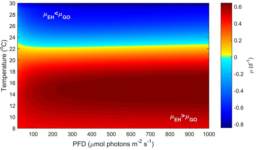
Figure 4. Predicted difference in growth rates between G. oceanica and E. huxleyi across a light range of 50–1000 µmol photons m−2 s−1
and a temperature range of 8–30 ◦ C at 400 µatm f CO2 based on Eq. (2).
4.4.2 Potentially realised niche are based on single-strain laboratory experiments, there is ev-
idence that such differences in temperature sensitivity may
Temperature and CO2 both have substantial effects on the also hold true in the modern ocean. For example, data gath-
potentially realised niche of E. huxleyi and G. oceanica ered from multiple phytoplankton monitoring cruises indi-
(Figs. 4 and 5). In contrast, light intensity has very little ef- cate that while both species are found at higher temperatures,
fect (Fig. 3). E. huxleyi appears able to exceed growth rates G. oceanica largely vanishes from the assemblage at temper-
of G. oceanica at temperatures below 22 ◦ C under most CO2 atures below 13 ◦ C (McIntyre and Bé, 1967; Eynaud et al.,
and light conditions (Figs. 4 and 5). A similar difference 1999; Hagino et al., 2005). However, phytoplankton moni-
in temperature preferences has also been observed in New toring cruises can be seasonally biased and represent a single
Zealand isolates of Gephyrocapsa oceanica and Emiliania point in time.
huxleyi with G. oceanica and E. huxleyi growing in the range Another way to relate our niche comparison to today’s
of 10–25 and 5–25 ◦ C at optimum temperatures of 22 and oceans is through surface sediments. Surface sediment sam-
20 ◦ C, respectively (Rhodes et al., 1995). While these results
www.biogeosciences.net/15/3541/2018/ Biogeosciences, 15, 3541–3560, 20183552 N. A. Gafar and K. G. Schulz: Niche comparison of E. huxleyi and G. oceanica
Figure 5. Predicted difference in growth rates between E. huxleyi and G. oceanica across a temperature range of 8–30 ◦ C and a f CO2 range
of 25–4000 µatm at 150 µmol photons m−2 s−1 of light based on Eq. (2).
10
8
6
log(EHGO ratio)
4
2
0
Pacific
-2 Atlantic A
Atlantic B
Indian
-4 Mediterranean
South China
-6
0 5 10 15 20 25 30
Temperature o C
Figure 6. Log ratio of E. huxleyi to G. oceanica coccoliths versus temperature in the global oceans. Symbols and colours represent different
ocean basins with data taken from McIntyre and Bé (1967), Chen and Shieh (1982), Roth and Coulbourn (1982), Knappertsbusch (1993),
Andruleit and Rogalla (2002), Boeckel et al. (2006), Fernando et al. (2007) and Saavedra-Pellitero et al. (2014). Symbols denote samples
from different oceanic regions with Atlantic B specifically representing samples from Boeckel et al. (2006) which appear influenced by
upwelling of nutrients (see Sect. 4.4.2), while Atlantic A refers to samples from the Atlantic ocean from all other studies. The line at zero
indicates a shift in dominance from E. huxleyi (> 0) to G. oceanica (< 0). The grey line represents a linear regression through the entire dataset
with p < 0.05 and F of 156.05 with 95 % prediction bounds for new observations. For details, see Sect. 2.9.
ples represent an integrated signal of the composition of a Boeckel et al. (2006) do not follow the general temperature
phytoplankton community over time and can therefore be a trend observed in other ocean basins (Fig. 6). In this loca-
more suitable proxy of species dominance in a certain lo- tion, it appears that G. oceanica abundance is driven more
cation. Global surface sediment data on G. oceanica and E. by increasing nutrient concentrations than by temperature.
huxleyi coccolith abundance indicate that the dominance of It seems oceanic upwelling in this region is driving a dif-
these two species is influenced by temperature, particularly ferent relationship between E. huxleyi and G. oceanica than
in the Pacific Ocean (Fig. 6). It is noted, however, that sam- observed in other areas. Globally, the data suggest that dom-
ples from the south-equatorial to equatorial Atlantic Ocean in inance switches from E. huxleyi to G. oceanica at tempera-
Biogeosciences, 15, 3541–3560, 2018 www.biogeosciences.net/15/3541/2018/N. A. Gafar and K. G. Schulz: Niche comparison of E. huxleyi and G. oceanica 3553
tures above 25 ◦ C which is similar to our projections. While tition for macro- or micronutrients (Zondervan, 2007; Mon-
both species have a similar upper limit to their fundamen- teiro et al., 2016; Browning et al., 2017). Thus, a potential
tal thermal niche (i.e. Rhodes et al., 1995), it would appear for high CaCO3 production is not necessarily realised when
that the higher minimum temperature of G. oceanica, com- exposed to different top-down and bottom-up pressures.
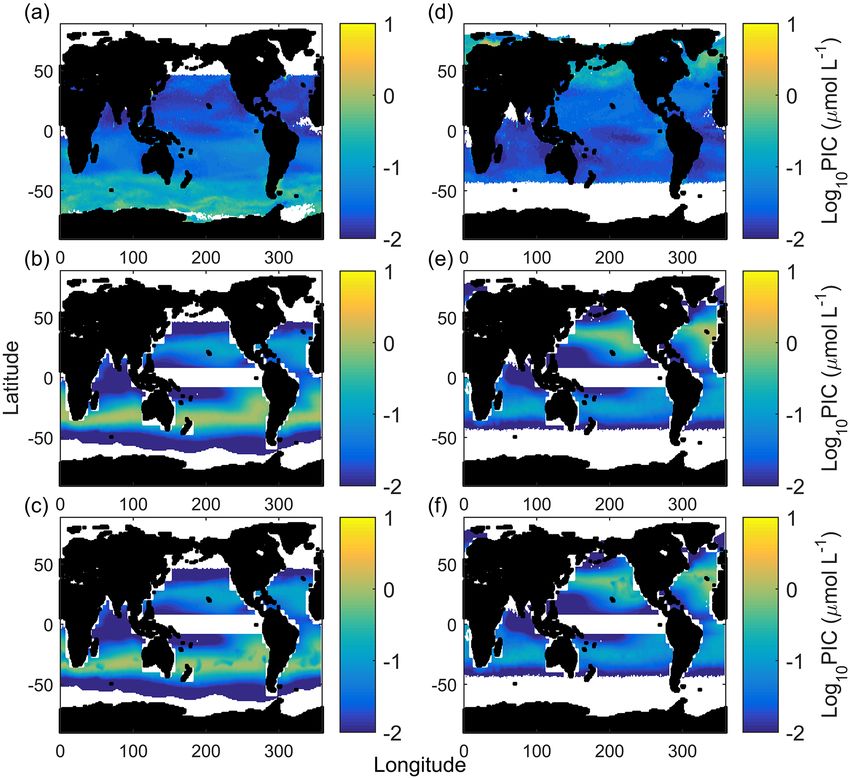
bined with its greater tolerance for high temperatures, re- Calculated CCPP of E. huxleyi alone (Fig. 7) for the
stricts its realised niche to the upper end of the temperature global ocean visually reproduces the midlatitude produc-
range (Figs. 4 and 6). tion belts, however at lower latitudes than satellite PIC es-
CO2 level also influences the relative growth rates of timates. This agrees with the NEMO and OCCAM mod-
E. huxleyi and G. oceanica. Under present-day levels of els of coccolithophore dominance (Sinha et al., 2010) and
∼ 400 µatm, E. huxleyi would dominate at temperatures up the chlorophyll a NASA Ocean Biogeochemical Model
to 22 ◦ C (Fig. 5). However, at higher and lower CO2 levels, (NOBM) model for the Southern Hemisphere and central
E. huxleyi begins to outgrow G. oceanica at progressively North Atlantic provinces (Gregg and Casey, 2007). CCPP
higher temperatures. At the same time, combined warming in also estimates seasonal changes with higher productivity dur-
a future ocean would partially mitigate the higher CO2 sen- ing summer in both hemispheres (see Fig. 7a and d vs. b and
sitivity of G. oceanica (Fig. 5). Nevertheless, over the natu- e). This pattern is driven mainly by temperature, which in-
rally observed temperature range, G. oceanica' s niche would fluences the latitudinal location of the bands, and light in-
be expected to decrease towards higher CO2 levels. tensity, which influences whether the northern or southern
This comparison only considers the responses of single band of productivity is stronger in a season. Nutrients are an
strains of E. huxleyi and G. oceanica. Considering multiple essential, and in the ocean often limiting, requirement for bi-
strains, from diverse ocean regions, would aid our study in ological productivity (Kattner et al., 2004; Browning et al.,
describing the fundamental and realised niches for a species 2017). As such, it would be expected that nutrients should
in more general terms. However, even though our realised also be strongly influencing seasonal patterns of PIC produc-
niche projections are based on only one strain for each tion. However, with the starting cell concentrations for the
species, they do generally agree with experimental observa- CCPP calculations chosen here, there was sufficient nitrate
tions of other strains and with planktonic and sediment obser- to support the projected production in most ocean regions
vations of each species as a whole. This indicates that the dif- (Fig. 7c and f). High temperatures drove relatively low pro-
ferences in requirements and sensitivities of the two species ductivity in the equatorial regions in agreement with satellite
as described here are large enough to be revealed by choosing PIC. Similar low levels of coccolithophores are estimated in
only one representative for each species. Another considera- Sinha et al. (2010) in the equatorial Pacific and Atlantic with
tion to be made is the fact that coccolithophore communities the mixed phytoplankton functional group dominating with
can be made up of dozens of species (McIntyre and Bé, 1967; or without coccolithophores due to low iron and moderate
Winter and Siesser, 1994), all of which are likely to have dif- phosphate concentrations, and in Gregg and Casey (2007)
ferent preferences for and sensitivities to changes in f CO2 , for the equatorial Indian and Atlantic provinces. CCPP un-
temperature and light. Shifts in plankton community struc- derestimates production at cold high latitudes, in particular
ture, as a result of different species and group preferences, in the Southern Ocean, when compared to the satellite. Simi-
in response to environmental change have already been ob- lar low levels of coccolithophores have been projected in the
served in the past (Beaugrand et al., 2013; Rivero-Calle et al., Southern Ocean in Gregg and Casey (2007) (very low coc-
2015), while simulations also suggest shifts in plankton com- colithophore chlorophyll a), Krumhardt et al. (2017) (growth
munity under future climate conditions (Dutkiewicz et al., rates at or close to zero which equates to low to zero CCPP)
2015). Community structure shifts and changes in coccol- and Sinha et al. (2010) (high nutrients resulting in coccol-
ithophore species composition are likely to alter ocean bio- ithophores being dominated by diatoms). For the Southern
geochemistry with implications for ocean-atmosphere CO2 Ocean, it has been suggested that satellite PIC concentra-
partitioning. tions in subantarctic waters are overestimated by a factor of
2–3 while those in Antarctic waters may be even more so
4.5 Global calcium carbonate production potential (Holligan et al., 2010; Balch et al., 2011; Trull et al., 2018).
The fact that three other global estimates, based on different
The CCPP is based on cellular CaCO3 quotas and growth sets of environmental parameters, all estimate very little PIC
rates calculated for a given set of temperature, light and car- productivity in the Southern Ocean seems to support this the-
bonate chemistry conditions (see Sect. 2.10). Here, we test ory. However, there are also specifically cold-adapted strains
how this measure for productivity compares to estimated of Emiliania huxleyi found at high latitudes which at least
surface ocean CaCO3 content observed by satellite imag- partially could explain discrepancies between the mentioned
ing (PICs ). At this point, it is important to remember that model projections and satellite-derived PIC concentrations
CCPP does not account for top-down controls such as graz- (see also below).
ing or viral attack (Holligan et al., 1993; Wilson et al., 2002; In austral winter/boreal summer, CCPP (for E. huxleyi)
Behrenfeld, 2014), and bottom-up controls such as compe- and satellite PIC estimates closely match (R 2 of 0.73, F of
www.biogeosciences.net/15/3541/2018/ Biogeosciences, 15, 3541–3560, 2018You can also read