Impact of tidal dynamics on diel vertical migration of zooplankton in Hudson Bay - Ocean Sciences
←
→
Page content transcription
If your browser does not render page correctly, please read the page content below
Ocean Sci., 16, 337–353, 2020
https://doi.org/10.5194/os-16-337-2020
© Author(s) 2020. This work is distributed under
the Creative Commons Attribution 4.0 License.

Impact of tidal dynamics on diel vertical migration of
zooplankton in Hudson Bay
Vladislav Y. Petrusevich1 , Igor A. Dmitrenko1 , Andrea Niemi2 , Sergey A. Kirillov1 , Christina Michelle Kamula1 ,
Zou Zou A. Kuzyk1 , David G. Barber1 , and Jens K. Ehn1
1 University   of Manitoba, Centre for Earth Observation Science, Winnipeg, Canada
2 Fisheries   and Oceans Canada, Winnipeg, Manitoba, Canada

Correspondence: Vladislav Y. Petrusevich (vlad.petrusevich@umanitoba.ca)

Received: 27 September 2019 – Discussion started: 7 October 2019
Revised: 30 January 2020 – Accepted: 7 February 2020 – Published: 17 March 2020

Abstract. Hudson Bay is a large seasonally ice-covered           1   Introduction
Canadian inland sea connected to the Arctic Ocean and North
Atlantic through Foxe Basin and Hudson Strait. This study
investigates zooplankton distribution, dynamics, and factors     The diel vertical migration (DVM) of zooplankton is a syn-
controlling them during open-water and ice cover periods         chronized movement of individuals through the water col-
(from September 2016 to October 2017) in Hudson Bay. A           umn and is considered to be the largest daily synchronized
mooring equipped with two acoustic Doppler current profil-       migration of biomass in the ocean (Brierley, 2014). This
ers (ADCPs) and a sediment trap was deployed in Septem-          migration is majorly controlled by two biological factors:
ber 2016 in Hudson Bay ∼ 190 km northeast from the port          (1) predator avoidance by staying away from the illuminated
of Churchill. The backscatter intensity and vertical veloc-      surface layer during the day and thus reducing the light-
ity time series showed a pattern typical for zooplankton diel    dependent mortality risk (Hays, 2003; Ringelberg, 2010;
vertical migration (DVM). The sediment trap collected five       Torgersen, 2003) and (2) optimization of feeding, with the
zooplankton taxa including two calanoid copepods (Calanus        assumption that algal biomass is greater in the surface layer
glacialis and Pseudocalanus spp.), a pelagic sea snail (Li-      during evening hours and zooplankton rise to feed on it in the
macina helicina), a gelatinous arrow worm (Parasagitta ele-      evening (Lampert, 1989). There are three general DVM pat-
gans), and an amphipod (Themisto libellula). From the ac-        terns: (1) the most common one is nocturnal when zooplank-
quired acoustic data we observed the interaction of DVM          ton ascend around sunset and remain at upper depths during
with multiple factors including lunar light, tides, and water    the night, descending around sunrise and remaining at depth
and sea ice dynamics. Solar illuminance was the major factor     during the day (Cisewski et al., 2010; Cohen and Forward,
determining migration pattern, but unlike at some other po-      2002). (2) Then there is a reverse pattern when zooplankton
lar and subpolar regions, moonlight had little effect on DVM,    ascend at dawn and descend at dusk (Heywood, 1996; Pas-
while tidal dynamics are important. The presented data con-      cual et al., 2017). And finally, (3) there is a twilight DVM
stitute the first-ever observed DVM in Hudson Bay during         pattern when zooplankton ascend at sunset, descend around
winter and its interaction with the tidal dynamics.              midnight, ascend again, and finally descend at sunset (Cohen
                                                                 and Forward, 2005; Valle-Levinson et al., 2014). This pat-
                                                                 tern is sometimes called midnight sink. DVM of zooplank-
                                                                 ton is an important process of the carbon and nitrogen cycle
                                                                 in marine systems because it effectively acts as a biological
                                                                 pump, transporting carbon and nitrogen vertically below the
                                                                 mixed layer by respiration and excretion (Darnis et al., 2017;
                                                                 Doney and Steinberg, 2013; Falk-Petersen et al., 2008). The
                                                                 following research question needs to be addressed: what sets

Published by Copernicus Publications on behalf of the European Geosciences Union.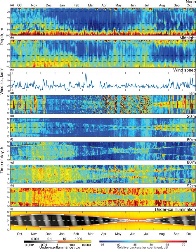
338                             V. Y. Petrusevich et al.: Impact of tidal dynamics on diel vertical migration of zooplankton

the timing of this synchronized movement in the Arctic envi-           In this study, factors controlling zooplankton distribution
ronment? Earlier studies of DVM in the Arctic were focused          during the open-water and ice-covered periods are investi-
on the period of midnight sun or the transition period from         gated using ADCP data together with sediment trap samples
midnight sun to a day–night cycle (Blachowiak-Samolyk et            for the first time in Hudson Bay. The main objectives are to
al., 2006; Cottier et al., 2006; Falk-Petersen et al., 2008;        (1) examine DVM during open-water and ice-covered sea-
Fortier et al., 2001; Kosobokova, 1978; Rabindranath et al.,        sons in Hudson Bay in 2016–2017, (2) identify zooplank-
2010). Recent studies based on acoustic backscatter data and        ton species involved in DVM, and (3) describe the DVM re-
zooplankton sampling showed the presence of synchronized            sponse to solar and lunar light, tides, and water and sea ice
DVM behavior continuing throughout the Arctic winter, dur-          dynamics.
ing both open and ice-covered waters (Båtnes et al., 2015;
Benoit et al., 2010; Berge et al., 2009, 2012, 2015a, b; Co-
hen et al., 2015; Last et al., 2016; Petrusevich et al., 2016;      2   Study area
Wallace et al., 2010). It was proposed that (Berge et al., 2014;
Hobbs et al., 2018; Last et al., 2016; Petrusevich et al., 2016),   Hudson Bay (Fig. 1a) is a large (with an area about
during polar night, DVM is regulated by diel variations in          831 000 km2 ) seasonally ice-covered shallow inland sea with
solar and lunar illumination, which are at intensities far be-      an average depth of 125 m and maximum depth below 300 m
low the threshold of human perception. Another reason for           (Burt et al., 2016; Ingram and Prinseberg, 1998; Macdon-
increasing interest in studying DVM patterns in various geo-        ald and Kuzyk, 2011; Petrusevich et al., 2018; St-Laurent et
physical and geographical environments and their seasonal           al., 2008; Straneo and Saucier, 2008). The seabed is charac-
changes in response to changing oceanographic conditions is         terized by fluted tills, postglacial infills, moraines, and sub-
that they could help inform us about physical oceanographic         glacial channels eroded to bedrock, resulting in bottom depth
processes. Furthermore, DVM patterns can be significantly           varying from 200 m to ∼ 10 m (Josenhans and Zevenhuizen,
modified by water column stratification (Berge et al., 2014)        1990). The tides are mostly lunar semidiurnal (M2 ) with an
and water dynamics, such as polynya-induced estuarine-like          amplitude of about 3 m at the entrance to Hudson Bay from
circulation (Petrusevich et al., 2016), tidal currents (Hill,       Hudson Strait (Prinsenberg and Freeman, 1986; St-Laurent et
1991, 1994; Valle-Levinson et al., 2014), and upwelling and         al., 2008) and about 1.5 m in Churchill (Prinsenberg, 1987;
downwelling (Dmitrenko et al., 2019; Wang et al., 2015).            Saucier et al., 2004; Ray, 2016) (Fig. 1). The marine water
   In the Arctic Ocean, the DVM process can be difficult            masses flow into Hudson Bay through two gateways: (1) the
to measure. However, there has been recent success in us-           Gulf of Boothia to Fury and Hecla Strait through Foxe Basin
ing data obtained by an acoustic Doppler current profiler           and (2) Baffin Bay to Hudson Strait (Fig. 1a). Measurements
(ADCP), which is a modern oceanographic instrument com-             of alkalinity and nutrient ratios suggest that the water masses
monly used to measure the vertical profile of current veloci-       within Hudson Bay are dominated by Pacific-origin waters
ties. Because the velocity profiling by an ADCP is based on         from the Arctic Ocean (Burt et al., 2016; Jones et al., 2003),
processing the measured intensity of acoustic pings backscat-       and the phytoplankton and zooplankton assemblages resem-
tered by suspended particles in the water column, further           ble those in the Arctic Ocean (Estrada et al., 2012; Runge and
processing of the measured acoustic backscatter to volume           Ingram, 1991). Freshwater inputs to Hudson Bay are very
backscatter strength (Deines, 1999) has been successful in          large, including river runoff from the largest watershed in
quantifying zooplankton abundance (Bozzano et al., 2014;            Canada, together with seasonal inputs of sea ice melt. The
Brierley et al., 2006; Cisewski et al., 2010; Cisewski and          freshwater inputs together produce strong stratification at the
Strass, 2016; Fielding et al., 2004; Guerra et al., 2019; Hobbs     surface in summer (Ferland et al., 2011). Fall storms and
et al., 2018; Last et al., 2016; Lemon et al., 2008; Petruse-       cooling, followed by brine rejection from sea ice formation
vich et al., 2016; Potiris et al., 2018, etc.). ADCP backscatter    during winter produces a winter surface mixed layer varying
data, validated using a time series of zooplankton samples          from ∼ 40 to > 90 m deep throughout Hudson Bay (Prinsen-
collected from sediment traps, provide a particularly useful        berg, 1987; Saucier et al., 2004).
tool for better understanding the effects of physical oceano-          Hudson Bay is ice-covered during 7–9 months a year, with
graphic processes on zooplankton DVM, changes in zoo-               ice formation typically starting in the northwest part of the
plankton community composition throughout the year, and             bay in late October (Hochheim and Barber, 2014). The mean
marine ecosystem function and carbon cycling (Berge et al.,         maximum ice thickness ranges from 1.2 m in the northwest to
2009; Willis et al., 2006, 2008).                                   1.7 m in the east (Landy et al., 2017). Around Churchill, the
   In this study, we are focused on zooplankton organisms           ice usually starts forming in October–November and breaks
with sizes from 500 µm and up. This group of zooplankton            up in May–June (Gagnon and Gough, 2005, 2006). Since
is primarily detected by ADCP backscatter (Cisewski and             1996 the open-water season has, on average, increased by 3.1
Strass, 2016; Pinot and Jansá, 2001) and allows for compari-        (±0.6) weeks in Hudson Bay, with mean shifts in dates for
son with previous studies on zooplankton caught by sediment         freeze-up and breakup of 1.6 (±0.3) and 1.5 (±0.4) weeks
traps (see Forbes et al., 1992; Pospelova et al., 2010).            accordingly (Hochheim and Barber, 2014).

Ocean Sci., 16, 337–353, 2020                                                                   www.ocean-sci.net/16/337/2020/
V. Y. Petrusevich et al.: Impact of tidal dynamics on diel vertical migration of zooplankton                                    339

Figure 1. (a) A bathymetric map of the Hudson Bay region and the location of the mooring (AN01). The inset map shows Hudson Bay on a
map of Canada. (b) Schematic illustration of the mooring AN01 setup.

   There have been few studies on zooplankton community             the port of Churchill (59◦ 58.1560 N 91◦ 57.1440 W) on
composition in Hudson Bay. Among the macrozooplankton               26 September 2016 and recovered on 30 October 2017.
species found in Hudson Bay, Parasagitta elegans is the most        The mooring setup consisted of (i) one upward-looking
abundant species, followed by Aglantha digitale as the sec-         five-beam Signature 500 ADCP by Nortek placed at
ond most abundant (Estrada et al., 2012). The mesoplankton          38 m of depth, (ii) an upward-looking four-beam 300 kHz
community in Hudson Bay is dominated by small copepods:             Workhorse Sentinel ADCP by RD Instruments placed
Oithona similis, Oncaea borealis, and Microcalanus (Estrada         at 106 m of depth, and (iii) one Gurney Instruments
et al., 2012). Zooplankton diversity is generally low at high       “Baker-type” sequential sediment trap (Baker and Milburn,
latitudes (Conover and Huntley, 1991). Typically, salinity          1983) at 85 m with a collection area of 0.032 m2 . Sev-
gradients and freshwater discharge play an important role           eral conductivity–temperature, conductivity–temperature–
in determining species diversity (Witman et al., 2008). Sea-        turbidity, and temperature–turbidity sensors were also de-
sonality in food availability is another significant challenging    ployed at various depths on the mooring, but the data ob-
factor for zooplankton in high latitudes (Bandara et al., 2016;     tained by these sensors were not analyzed in this study.
Carmack and Wassmann, 2006; Varpe, 2012).                              The velocity and acoustic backscatter (ABS) intensity
                                                                    were measured by a Teledyne RD Instruments (RDI) ADCP
                                                                    between 8 and 100 m at 2 m depth intervals, with a 15 min en-
3     Data collection and methods                                   semble time interval and 15 pings per ensemble. The ADCP
                                                                    velocity measurement precision and resolution were ±0.5 %
3.1    Mooring configuration and setup
                                                                    and ±0.1 cm s−1 , respectively. The accuracy of the ADCP
A bottom-anchored oceanographic mooring (Fig. 1b) was               vertical velocity measurements are not validated; however,
deployed at 109 m of depth ∼ 190 km northeast from                  the RDI reports that the vertical velocity is more accurate, by

www.ocean-sci.net/16/337/2020/                                                                     Ocean Sci., 16, 337–353, 2020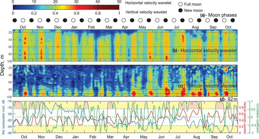
340 V. Y. Petrusevich et al.: Impact of tidal dynamics on diel vertical migration of zooplankton
at least a factor of 2, than the horizontal velocity (Wood and high albedo at visible wavelengths for snow-covered or white
Gartner, 2010). The compass accuracy was ±2◦ , and com- ice surfaces.
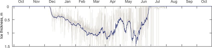
pass readings were corrected by adding magnetic declination. The thickness of (Fig. 2) ice at the mooring location was
The sediment trap was programmed to start a collec- estimated from the ice draft evaluated from the distance to the
tion at 4 October 2016 at 00:00 CST with intervals of 35 d ice–ocean interface measured by the Nortek ADCP (Banks
for each vial collected. Prior to boarding the vessel, sedi- et al., 2006; Björk et al., 2008; Shcherbina et al., 2005; Vis-
ment trap preservative density solution was prepared at the beck and Fischer, 1995). The draft was further transformed to
Churchill Northern Studies Centre (CNSC). To prepare the the ice thickness by multiplying by a factor of 1.115 for the
solution, 10 L of seawater was collected from the Churchill density difference between seawater and sea ice (Bourke and
port wharf and filtered through 0.7 µm Whatman GF/F fil- Paquette, 1989). The acoustic-derived thicknesses were cor-
ters. The salinity of the filtered seawater was adjusted from rected for ADCP tilt, sea surface height, atmospheric pres-
26.7 to 37 psu with 88.065 g of ultraclean sea salt. Borax sure (Krishfield et al., 2014), and the speed of sound. The
(44.4 g) was slowly added to 0.45 L of 37 % formaldehyde, extreme outliers were excluded, and the mean daily ice thick-
placed on a magnetic stir plate overnight to dissolve, and de- nesses were calculated for further analysis (Fig. 2).
canted into 8.55 L of filtered seawater. Approximately 1 h be- The Environment and Climate Change Canada weather
fore deployment of the sediment traps, pre-acid-cleaned vials station at Churchill airport (YYQ), located ∼ 190 km south-
were placed inside the preprogrammed sampling carrousel west from the mooring location, provided wind data for most
and filled to the surface with the preservative solution. The of the time of mooring deployment, except for the period
trap was assembled and kept upright prior to and during de- of 27 March–7 April 2017. The daily mean wind speed
ployment. During deployment, the different species of zoo- magnitude was used to compile the wind speed time series
plankton were captured by the sediment trap (Fig. 6). (Fig. 3c).
On recovery of the mooring, sediment trap samples were
3.2 Data collection and post-processing photographed, poured into acid-cleaned 250 mL amber glass
bottles, and stored in the dark at approximately 4 ◦ C during
ADCPs, unlike echo sounders (Lemon et al., 2012, 2001), are transport to the Centre for Earth Observation Science, Uni-
limited in deriving accurate quantitative estimates of biomass versity of Manitoba. Samples were poured through a 500 µm
due to calibration difficulties because their acoustic beams NITEX mesh sieve to separate the larger zooplankton frac-
are narrow and inclined from the vertical (Brierley et al., tion. The 500 µm mesh was selected to maintain consistency
1998; Lemon et al., 2008; Sato et al., 2013; Vestheim et al., and allow for comparison with previous studies (see Forbes
2014). But with the application of beam geometry correc- et al., 1992; Pospelova et al., 2010). Because of this, smaller
tion, ADCPs are commonly used for qualitative studies, as species, nauplii, eggs, and fecal pellets were largely missed
they can provide information on zooplankton presence and from the > 500 µm fraction. However, the > 500 µm organ-
behavior (Hobbs et al., 2018; Last et al., 2016; Petrusevich et isms represent the group of zooplankton primarily detected
al., 2016). To correct for the ADCP beam geometry, we de- as ADCP backscatter (Cisewski and Strass, 2016; Pinot and
rived the volume backscatter strength (VBS) Sv in decibels Jansá, 2001). Zooplankton taxonomy identification was con-
(dB) from echo intensity following the procedure described ducted at the Freshwater Institute (DFO) to the lowest taxo-
by Deines (1999). The issue of acoustic signal scattering by nomic level possible, enumerated, and measured. The entire
bubbles, waves, and sea ice was addressed by removing the sample was scanned for large and rare organisms and then the
top 8 m readings from all backscatter and velocity data. sample was split, with a Motoda box splitter, and a minimum
The total sky illumination for day and night was mod- of 300 organisms were counted for each sample.
eled using the skylight.m function from the astronomy
package for MATLAB (Ofek, 2014) and a simple exponen-
tial decay radiative transfer model for estimating under-ice
4 Results
illumination (Grenfell and Maykut, 1977; Perovich, 1996).
Transmittance through the sea ice was calculated following
4.1 Ice thickness and under-ice illumination
Eq. (1):
T (z) = (1 − α)e−kt z , (1) At the mooring location, the ice started rapidly forming in the
second week of December. By mid-December the thickness
where α is the surface albedo, κt is the bulk extinction coeffi- reached 0.4 m and gradually grew until the middle of March
cient of the sea ice cover, and z is the ice thickness. The val- up to 1 m (Fig. 2). Afterwards, the ice thickness at the moor-
ues of the coefficients used in the exponential decay model ing location varied due to seasonal factors, e.g., polynyas, sea
were adjusted for the first-year sea ice: α = 0.8 and κt = 1.2. ice melting, etc.
We did not have any data for snow cover available, so the Modeled under-ice illumination time series, as well as the
presence of snow cover was omitted in the transmittance volume backscatter strength and vertical velocity time series,
model. However, an albedo of 0.8 was used to simulate the were presented in the form of actograms (Figs. 3d–g and
Ocean Sci., 16, 337–353, 2020 www.ocean-sci.net/16/337/2020/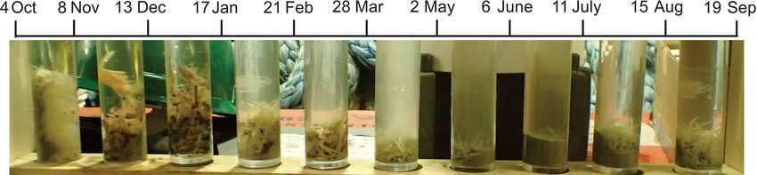
V. Y. Petrusevich et al.: Impact of tidal dynamics on diel vertical migration of zooplankton 341
Figure 2. ADCP-measured ice thickness at the mooring location (AN01) during winter 2016–2017. Gray and blue lines represent the filtered
and daily averaged ice thicknesses, respectively.
4). An actogram, being a common method of data display VBS was calculated for depths of 8, 20, 60, 80, and 92 m
in chronobiological research, has recently been used for dis- and is shown as actograms in Fig. 3d–h. Overall, VBS ac-
playing zooplankton DVM (Hobbs et al., 2018; Last et al., tograms show a similar shape as that of the under-ice solar
2016; Petrusevich et al., 2016; Tran et al., 2016). illumination actogram (Fig. 3i). This resemblance in shape is
The actogram of the modeled under-ice illumination outlined by reduced VBS at 8 and 20 m actograms (Fig. 3d–
(Figs. 3i and 4e) shows continuous daily maximums at noon, e) and enhanced at 60, 80, and 92 m actograms (Fig. 3f–
with minimum values of 2000 lx around the winter solstice h) during dawn and dusk. Reduced under-ice illumination
and maximum values of 10 000 lx in the middle of summer. from December to March corresponded with reduced VBS
Maximum under-ice lunar illumination was around 0.1 lx through the whole water column, followed by increased illu-
during a full moon under sea ice about 0.5 m thick. mination during ice breakup and open-water periods (April
to October) and an increase in VBS within all five depth
bins. Like the noon and midnight VBS time series, there
4.2 Volume backscatter strength (VBS) is a relatively higher signal at 60, 80, and 92 m of depth in
November–January during the night.
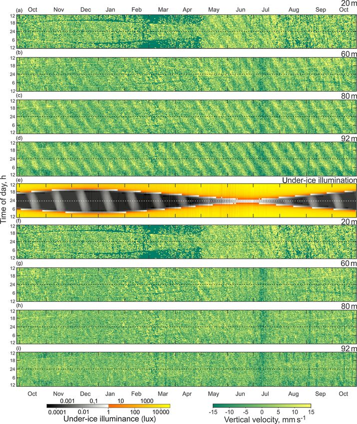
To analyze the depth-dependent behavior of scatterers in- The VBS actograms (Fig. 3d–h) show the presence of ver-
volved in diurnal vertical migration, we computed the vol- tical bands of higher VBS with 14 d periodicity at multiple
ume backscatter strength (VBS) time series at noon (Fig. 3a) depths. In the upper 8 and 20 m (Fig. 3d–e), these bands
and at midnight (Fig. 3b). The mean difference between spread through the night period, while at 80 and 92 m ac-
noontime and midnight VBS was ∼ 9±1 dB at the 96–100 m tograms the bands spread throughout the whole day, with
depth layer and −3 dB ± 1 at the 10–28 m layer. Running different values of VBS during the day and night. In the
an F -statistic test returned statistical significance with 95 % 8 m actogram (Fig. 3d) there are also nonperiodic bands of
confidence for the VBS difference below 58 m and above high backscatter that span from 1 to 5 d in duration. These
48 m. Noontime series show persistent maximum backscat- bands spread throughout the whole day and correspond to
ter strength near the bottom below 92 m of depth, which is the periods of wind speed increasing to strong wind, gale,
consistent with DVM. Some scatter stayed at noon at the 60– and storm values (30 km h−1 and up) during the ice-free sea-
80 m layer during October–January and at 70–80 m in June– son (Fig. 3c).
July. Figure 3c shows daily mean wind speed measured at
The near-bottom maximum for the midnight time series of Churchill airport (YYQ). There were several observed pe-
VBS is significantly lower compared to that for noon. Mid- riods of mean wind speed higher than 30 km h−1 , which
night time series during October–February and May–July corresponds to strong wind (37–61 km h−1 ) and gale (62–
showed a wider spread of scatterers over the depth. During 87 km h−1 ) wind speed values, with maximum wind gusting
winter months (December–February), the thickness of this up to 77 km h−1 . Normally these storm events lasted from 1
layer of midnight bottom scatterers gradually decreased with to 6 d.
the growth of sea ice. There are periods of higher VBS at the
bottom layer with the same periodicity of 14 d as the super- 4.3 Vertical velocity actograms
position maxima of the M2 and S2 tidal components (spring
tide) throughout the whole time series. There was a seasonal The vertical velocity actograms were calculated for the same
variation of these periodic VBS maxima: they increased dur- depths as VBS actograms (Fig. 4a–d). Positive velocities are
ing summer–fall and decreased in winter. It should be noted associated with the upward movement of particles. The sea-
that during November–January there were higher values of sonal shape of vertical velocity actograms is similar to the
backscatter below 80 m of depth. shape of under-ice illumination (Figs. 3c and 4e) and VBS
www.ocean-sci.net/16/337/2020/ Ocean Sci., 16, 337–353, 2020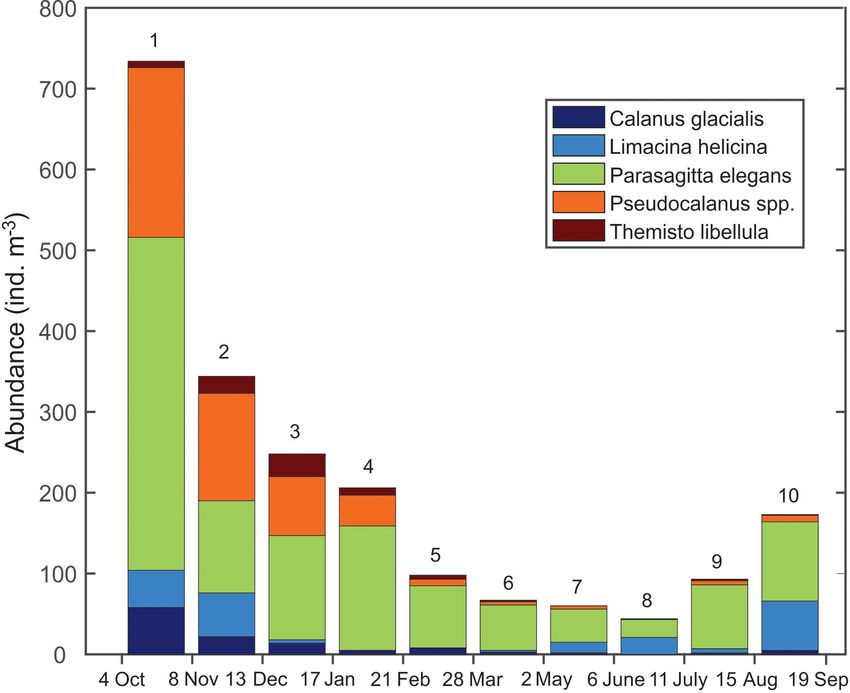
342                              V. Y. Petrusevich et al.: Impact of tidal dynamics on diel vertical migration of zooplankton

Figure 3. Time series (October 2016 to October 2017) of the (a) ADCP acoustic volume backscatter coefficient at noon and (b) at midnight,
(c) daily mean wind speed measured at Churchill airport (YYQ), and (d)–(i) actograms of ADCP acoustic backscatter at five depth levels:
(d) 8 m, (e) 20 m, (f) 60 m, (g) 80 m, and (h) 92 m, as well as (i) modeled under-ice illuminance. Dashed horizontal lines represent astronom-
ical midnight. The diurnal signal is presented at the vertical axis, while the long-term changes in diurnal behavior are presented along the
horizontal axis.

Ocean Sci., 16, 337–353, 2020                                                                           www.ocean-sci.net/16/337/2020/
V. Y. Petrusevich et al.: Impact of tidal dynamics on diel vertical migration of zooplankton                                                  343

Figure 4. Actograms of (a–d) ADCP-measured vertical velocity (mm s−1 ) at four depth levels: (a) 20 m, (b) 60 m, (c) 80 m, and (d) 92 m.
(e) Modeled under-ice illuminance and (f–i) residual vertical velocity (mm s−1 , tidal signal subtracted) at four depth levels: (f) 20 m, (g) 60 m,
(h) 80 m, and (i) 92 m. Positive and negative values correspond to the upward and downward net flux. Dashed horizontal lines represent
astronomical midnight.

www.ocean-sci.net/16/337/2020/                                                                                Ocean Sci., 16, 337–353, 2020
344                            V. Y. Petrusevich et al.: Impact of tidal dynamics on diel vertical migration of zooplankton

actograms (Fig. 3d–g). The change in vertical speed associ-       ing two calanoid copepods (Calanus glacialis and Pseu-
ated with spring tide is present on the vertical velocity ac-     docalanus spp.), a pelagic sea snail (Limacina helicina), a
tograms in the form of slanted strips of 14 d periodicity, with   gelatinous arrow worm (Parasagitta elegans), and an amphi-
amplitude increasing with depth and reaching maximum val-         pod (Themisto libellula) (Table 1, Fig. 7). The abundance of
ues in the range of 10–15 mm s−1 .                                organisms in the trap was generally lowest from March to
   The vertical velocity actograms were post-processed            July with the exception of juvenile (2 mm length) T. libellula
(Fig. 4f–i) to remove the semidiurnal tidal components (M2        in bottle 6.
and S2 ) from the vertical velocity data, which would other-
wise create a tidal background signal in the form of slanted
strips of 14 d periodicity on the actograms (Fig. 4a–d). A        5     Discussion
tidal harmonic analysis was performed for the vertical veloc-
ity time series using T_Tide toolbox for MATLAB (Pawlow-          5.1    Zooplankton species associated with DVM in
icz et al., 2002). There was a small distinguishable diurnal             Hudson Bay
variation of vertical velocity in the 20 and 60 m actograms
(Fig. 4f and g) during the period of the full moon in Octo-       The presence of seasonal ice cover acts as a barrier to us-
ber, November, and December resembling the slanted shape          ing traditional zooplankton sampling techniques. But using
of lunar illumination on the under-ice illumination actogram      both moored and ice-tethered ADCPs in high latitudes has
(Fig. 4e).                                                        been successful for studying zooplankton presence, behavior,
                                                                  and particularly DVM patterns (Darnis et al., 2017; Hobbs
4.4   Wavelet analysis                                            et al., 2018; Petrusevich et al., 2016; Wallace et al., 2010).
                                                                  Even though acoustic backscatter from the single-frequency
Time series of the wavelet power spectrum for the semidiur-       ADCP does not provide any information on the identity of
nal tidal currents were computed to account for their spring–     zooplankton species involved in DVM, signal strength can
neap and seasonal variability. Wavelets for horizontal and        provide an indication of zooplankton presence provided there
vertical velocities (Fig. 5b and c) show absolute maximum         is information on the zooplankton species. Sound is effec-
values during spring tides, which is consistent with the full     tively scattered by objects of the size of the wavelength. For
moon and new moon phases (Fig. 5a). The power spectrum            300 kHz ADCP, it is about 5 mm. It is known that zooplank-
range for horizontal velocities was in general over 1 order of    ton species with a body size less than the wavelength by an
magnitude higher than for vertical velocity, which is consis-     order of magnitude (in our case 0.5–5 mm) are capable of
tent with the fact that horizontal tidal currents tend to be at   creating strong backscatter when there is a sufficient abun-
least an order of magnitude larger than vertical ones. There      dance of them in the water column (Cisewski and Strass,
is a spatial difference between the horizontal and vertical ve-   2016; Pinot and Jansá, 2001). The backscatter strength of
locity power spectrum. The horizontal velocity wavelet has        zooplankton species also depends on their acoustic proper-
maximums that spread through the whole water column dur-          ties, such as shape, internal structure, orientation in the wa-
ing the ice-free season and below 30 m of depth in the pres-      ter column, and body composition, which causes a differ-
ence of ice cover (December–April). The vertical velocity         ence between the speed of sound in their bodies and the sur-
spectrum during October–April has maximums mostly con-            rounding seawater (Stanton et al., 1994, 1998a, b). For ex-
centrated below 70 m of depth. There is a seasonal varia-         ample, the species with hard shells (like Limacina helicina)
tion for the vertical velocity wavelet, with May–June wavelet     and gaseous enclosures scatter sound stronger than gelati-
maximums starting to spread through the whole water col-          nous ones (Lavery et al., 2007; Warren and Wiebe, 2008). It
umn.                                                              should be mentioned that 300 kHz ADCP can be effectively
   For the analysis of ADCP-measured current velocities, we       used for suspended sediment transport monitoring (Venditti
used wavelet transformation to derive the time-dependent          et al., 2016), but here are some general considerations that
behavior of horizontal and vertical current velocities at         need to be taken into account: 300 kHz ADCPs are used for
the semidiurnal tidal frequency band that dominates the           suspended sediment monitoring, mostly in rivers with high
backscatter spectrum. In this study, we used the generalized      sediment loads (hundreds of milligrams per liter). Our moor-
Morse wavelet (with parameters β = 100 and γ = 3) and             ing was located ∼ 190 km northeast from the Churchill River,
jWavelet toolbox (part of jLab toolbox) for signal process-       which does not create a significant plume of sediment into
ing (Lilly, 2017, 2019; Lilly and Gascard, 2006; Lilly and        the system. The mooring turbidity sensor located at 41 m of
Olhede, 2009).                                                    depth did not record values higher than 34 FTU, which cor-
                                                                  responds to TSS of ∼ 30 mg L−1 , with an average turbidity
4.5   Sediment trap zooplankton                                   of 7 FTU; this corresponds to TSS ∼ 5 mg L−1 . At 100 m of
                                                                  depth, we do not expect high levels of sediment from resus-
Zooplankton > 500 µm captured in the sediment trap sam-           pension. Also taking into consideration the fact that sound is
ples (Fig. 6) were dominated (> 98 %) by five taxa includ-        effectively scattered by objects of the size of the wavelength

Ocean Sci., 16, 337–353, 2020                                                                 www.ocean-sci.net/16/337/2020/
V. Y. Petrusevich et al.: Impact of tidal dynamics on diel vertical migration of zooplankton 345 Figure 5. Time series of (a) lunar phases for 2016–2017. : Full moon. •: New moon. (b, c) The absolute value of the wavelet power spectrum for the time series of horizontal velocity (b) and vertical velocity (c) computed for the semidiurnal frequency band (12 h) as a function of depth. (d) The correlation coefficient (green line) between time series of VBS (blue line) and the vertical velocity wavelet (red line) at 92 m of depth. Yellow shading identifies the correlation coefficient levels exceeding ±0.53, which are statistically significant for the 95 % confidence level. Pink shading identifies the events during which this statistically significant correlation was observed. Figure 6. Contents of the sediment trap for 10 intervals of 35 d. and that the mean particle size detected by 300 kHz ADCP et al., 2016) and Baffin Bay (LeBlanc et al., 2019). How- is in the range of 0.5 to 5 mm (Jourdin et al., 2014), sporadic ever, there is little known for Hudson Bay. It is expected that smaller scatterers, like sediment and phytoplankton, can ef- Hudson Bay Arctic cod behave similarly, with adult aggre- fectively be eliminated as potential scatterers. This allows us gations near the bottom in deep waters and young (year 1–2) to consider zooplankton to be the main scatterers in our case. and larval stages in surface aggregations. The young cod are Fish also can be detected with the ADCP used. It should ice-associated during the winter period, i.e., no migration to be noted though that large mesopelagic fishes are rare in depth. As such, any backscatter associated with near-surface the Canadian Arctic (Berge et al., 2015b). Arctic cod (Bore- young cod would have been removed as part of the removal ogadus saida) is the dominant pelagic fish in the Canadian of the top 8 m of backscatter during post-processing. Arctic Arctic (e.g., Benoit et al., 2008; LeBlanc et al., 2019), and cod do not school. So, its presence in the proximity of the therefore the acoustic signals related to fish are generally mooring will be more sporadic, and acoustic backscatter will assumed to be only Arctic cod. The distribution of Arctic be significantly less than the backscatter from much more cod is known for regions such as the Beaufort Sea (Geoffroy abundant zooplankton. www.ocean-sci.net/16/337/2020/ Ocean Sci., 16, 337–353, 2020
346                              V. Y. Petrusevich et al.: Impact of tidal dynamics on diel vertical migration of zooplankton

Table 1. Abundance (ind. m−3 ) and length (mm) of the dominant zooplankton (> 500 µm) in each bottle of the sediment trap at AN01 from
October 2016 to August 2017. Note: T. libellula juveniles and adults are presented separately for bottle 6; adult abundance and length are in
parentheses.

                   Trap bottle     Collection interval   Calanus      Limacina     Parasagitta    Pseudocalanus      Themisto
                                             (dd/mm)     glacialis     Helicina       elegans               spp.      libellula
              1      Abundance           04/10–08/11            58            46          412                210             8
                     Length                              3.2 ± 0.4     1.0 ± 0.5      23 ± 1.8          1.0 ± 0.2    8.3 ± 1.1
              2      Abundance           08/11–13/12            22            54          114                133            21
                     Length                              3.3 ± 0.5     1.0 ± 0.3      23 ± 2.0          1.2 ± 0.2     20 ± 1.3
              3      Abundance           13/12–17/01            14            4           129                  73           28
                     Length                              3.5 ± 0.7   0.8 ± 0.04       24 ± 1.6          1.1 ± 0.2     21 ± 1.6
              4      Abundance           17/01–21/02             5             0          154                  38            9
                     Length                              3.4 ± 0.2                    24 ± 2.0          1.0 ± 0.3     20 ± 1.7
              5      Abundance           21/02–28/03             8             0            77                  8            5
                     Length                              3.3 ± 0.4                    24 ± 2.1          1.3 ± 0.0     27 ± 4.8
              6      Abundance           28/03–02/05             3             2            56                  4      191 (2)
                     Length                              3.4 ± 0.2     1.1 ± 0.1      25 ± 1.9          0.8 ± 0.2       2 (22)
              7      Abundance           02/05–06/06             2            13            41                  4            0
                     Length                              3.8 ± 0.4     1.2 ± 0.0      26 ± 3.0          0.9 ± 0.1
              8      Abundance           06/06–11/07             0            21            22                  1            0
                     Length                                            1.6 ± 0.3      27 ± 1.9                1.3
              9      Abundance           11/07–15/08             2             5            79                  5            2
                     Length                              3.6 ± 0.1     1.5 ± 0.5      26 ± 2.5          1.1 ± 0.2     11 ± 3.5
              10     Abundance           15/08–19/09             5            61            98                  8            1
                     Length                              3.4 ± 0.8     1.1 ± 0.0      24 ± 2.2          1.1 ± 0.1           15

                                                                            The trap samples reflect the presence of > 500 µm zoo-
                                                                         plankton in the water column during the annual cycle. How-
                                                                         ever, the absence of a species from the trap samples (e.g.,
                                                                         L. helicina in January–March) does not confirm its absence
                                                                         from the water column. The most abundant species from
                                                                         the zooplankton trap catch (Parasagitta elegans, Pseudo-
                                                                         calanus, and L. helicina) had lengths of 20–30, 0.6–1.4,
                                                                         and 0.4–2 mm, respectively. Less abundant species from the
                                                                         trap (Calanus glacialis and Themisto libellula) had lengths
                                                                         of 2.8–4.2 and 7.2–31.8 mm, respectively. P. elegans and
                                                                         T. libellula lengths are in the range of ADCP wavelength
                                                                         and should thus effectively act as scatterers. Lengths of
                                                                         C. glacialis, Pseudocalanus, and L. helicina are less than
                                                                         the wavelength by an order of magnitude. However, their
                                                                         abundance in the water column during the open-water sea-
                                                                         son (Estrada et al., 2012) is high enough (> 1000 ind m3 ) to
                                                                         expect a backscatter signal. L. helicina’s hard shell should
                                                                         be another contributing factor to backscatter strength. There-
                                                                         fore, we assume that all the species identified in the sediment
Figure 7. Abundance (ind. m−3 ) of the dominant zooplankton (>           trap could act as acoustic scatterers contributing to the VBS
500 µm) in each bottle of the sediment trap at AN01 from Octo-           signal analyzed in this study.
ber 2016 to August 2017.
                                                                            The zooplankton caught in our sediment trap provide gen-
                                                                         eral information on the zooplankton community composition

Ocean Sci., 16, 337–353, 2020                                                                          www.ocean-sci.net/16/337/2020/
V. Y. Petrusevich et al.: Impact of tidal dynamics on diel vertical migration of zooplankton 347
and its change over the course of the year near the moor- gions where DVM was observed. In those locations, DVM
ing location. Sediment trap samples may not quantitatively during the winter was primarily controlled by twilight and
reflect zooplankton composition in the water column due the lunar light (Last et al., 2016; Petrusevich et al., 2016).
to species-specific collection efficiencies. Comparisons be- In this study, DVM was generally controlled by solar illumi-
tween net and trap samples from Franklin Bay indicate that nation throughout the whole year, which is evident from the
the abundance of L. helicina and some species of copepods shape of the VBS (Fig. 3d–h) and vertical velocity actograms
could be estimated from sediment traps, whereas the abun- (Fig. 4). The actograms are nearly symmetric around astro-
dance of other key species, such as C. hyperboreus, could not nomic midnight (dashed horizontal line, Figs. 3 and 4) and
be accurately estimated from sediment trap samples (Makabe the winter and summer solstice. During dawn and dusk, there
et al., 2016). was reduced VBS on the 8 and 20 m actograms (Fig. 3d–
The ADCP analysis indicates that zooplankton in Hud- e) and enhanced VBS on the 60, 80, and 92 m actograms
son Bay undergo both seasonal and diel migration. This is (Fig. 3f–h). These dawn and dusk absences and enhance-
similar to measured seasonal migration by copepod species ments can be interpreted as an indication of zooplankton
in the southern Arctic Ocean and in Rijpfjorden in Svalbard swimming behavior during these periods, following a noc-
(Falk-Petersen et al., 2008). Seasonal migration is occurring turnal DVM pattern. The increased backscatter at dawn and
in Hudson Bay despite shallower overwintering waters than dusk on the 60 and 80 m actograms was observed regardless
in Svalbard and the Beaufort Sea. The observed diel migra- of the presence of ice cover.
tion in Hudson Bay is similar to other Arctic locations (Berge The noontime VBS time series showed consistent max-
et al., 2014, 2015b; Hobbs et al., 2018; Last et al., 2016; imum backscatter strength below 92 m of depth (Fig. 3a).
Petrusevich et al., 2016), suggesting that DVM is an impor- Compared to the midnight time series (Fig. 3b), it is clear
tant consideration for carbon–nitrogen transfer within the rel- that the backscatter was associated with DVM rather than
atively shallow Hudson Bay system. sediment resuspension caused by the lunar semidiurnal M2
Zooplankton species identified from the sediment trap sug- tide with a period of 12 h 25 min. The midnight VBS time
gest that multiple species could be involved in the DVM. The series (Fig. 3b) and VBS actograms (Fig. 3d–h) confirm that
identification of individual species involved in DVM is not the zooplankton were aggregated in the upper water column
currently possible and is challenged by issues such as the at midnight, likely feeding.
overlapping of signals. Comparison between acoustic and net Seasonal variations in zooplankton migration and distribu-
data in Kongsfjorden, Svalbard, led to the conclusion that tion in the water column were observed throughout the entire
the acoustic backscatter signal from numerically dominant time series. The sediment trap at 85 m of depth may have cap-
Calanus copepods is typically overwhelmed by the signal tured zooplankton species migrating vertically and possibly
from larger and less abundant zooplankton species, such as also individuals sinking to the bottom (Fig. 6). The strong
Themisto (Berge et al., 2014). Large copepods (like Calanus VBS of −70 dB during noon at the 90–100 m depth layer
spp.) and chaetognaths (P. elegans) were observed perform- (Fig. 3a), compared with −80 dB at midnight (Fig. 3b), sug-
ing diel migrations in Kongsfjorden (Darnis et al., 2017). gests that noontime DVM-associated zooplankton biomass
While our sediment trap showed the prevalence of gelatinous was primarily located at the bottom layer through the an-
zooplankton species (Fig. 7 – P. elegans), the detection of nual cycle. From October to the middle of January, however,
their migration by ADCP backscattering could be underesti- there was a layer of VBS in the range of −80 to −75 dB
mated because gelatinous species are weak scatterers. at 60–80 m of depth, which can be interpreted as some of
Regardless, there is a pump of carbon–nitrogen occurring the zooplankton staying at that depth instead of migrating
within Hudson Bay based on zooplankton DVM, and sea- all the way down to the bottom for daytime or to the sur-
sonal differences (discussed in the next section) could im- face at night. The 60–80 m aggregation of zooplankton from
pact this vertical transport of elements. The collected acous- October to January corresponds to the first three sampling
tic data at hand are not valid to quantify zooplankton biomass bottles of the sediment trap when the highest abundance of
involved in DVM. However, we can use them to document zooplankton was observed with the abundance of dominant
and better understand important aspects of DVM, such as species per 35 d sampling period, decreasing from 720 down
links between its seasonal cycle and the dynamics of sea to 250 ind. m−3 (Fig. 7). From the middle of January to early
ice cover and under-ice illuminance, as well as the effects May, most of the zooplankton biomass at midnight did not
of windstorms and tides on DVM patterns. migrate above 60 m of depth. From May to July zooplank-
ton returned to the vertical migration pattern observed when
5.2 DVM seasonal cycle, sea ice cover, and under-ice zooplankton remain near the bottom at noon and migrate to
illuminance the surface at night. In July, some zooplankton stayed in the
surface layer at noon. This corresponds to the beginning of
The mooring site is located 6◦ south of the Arctic Circle and the ice-free season (Fig. 2) when long periods of daylight and
polar twilight zone. Hudson Bay is located more south than the abundance of phytoplankton disrupts DVM. Once the sea
other seasonally sea-ice-covered Arctic and sub-Arctic re- ice was completely gone in early August, there was a change
www.ocean-sci.net/16/337/2020/ Ocean Sci., 16, 337–353, 2020348 V. Y. Petrusevich et al.: Impact of tidal dynamics on diel vertical migration of zooplankton
in zooplankton distribution in the water column. During mid- new moon phases (Fig. 5a). For the 92 m depth, the 14 d run-
night, some zooplankton remained at the bottom, while oth- ning correlation (Fig. 5d, green line) between midnight VBS
ers migrated to the surface layer, likely feeding during the (blue line) and the vertical velocity wavelet (red line) was
short night and moving back down to the bottom for the light calculated. Correlations exceeding ±0.53 are statistically
time. This suggests that different zooplankton scatter species significant at the 95 % confidence level (Fig. 5d, yellow shad-
and/or size classes are responding differently to both solar ing). Pink shading identifies events during which this statis-
cues and ice cover. tically significant positive correlation was observed. Nega-
In certain cases vertical velocity actograms can be used to tive correlations are artificial and have no physical meaning.
estimate swimming direction and velocity (Petrusevich et al., The periods of low correlation were from the end of Novem-
2016), for example when actograms are averaged for layers ber to mid-January, mid-February to mid-March, April to
several meters deep for the estimation of swimming direc- mid-June, and the first half of September. A statistically sig-
tion and when individual profiles are averaged over a period nificant positive correlation suggests a relationship between
of a few days for velocity estimation. This method works VBS and tidal forcing.
well when there is no tidal signal to be subtracted from the In the presence of background stratification, the barotropic
vertical velocity data; otherwise, it makes computation rather tide interacts with sloping bottom topography in the proxim-
complicated. ity of the mooring location (Fig. 1), which is typical for Hud-
son Bay (Petrusevich et al., 2018). This interaction generates
5.3 Masking of DVM signal in the upper layer by the vertical divergence and convergence of tidal flow, result-
storms ing in the depth-dependent behavior of the vertical velocity
at a tidal frequency defined here as the baroclinic tide. The
The 8 m depth actogram (Fig. 3d) shows several bands of seasonal character of the baroclinic tide can also be affected
higher VBS of different durations that are not observed at by density stratification. During May–October 2017 the ver-
the deeper layers. These bands spread throughout the en- tical velocity wavelet maximums were amplified (Fig. 5c).
tire 24 h day for a duration of one to several days. These During this period there were DVM disruptions throughout
bands (Fig. 3d) nicely correspond to daily mean wind speed the water column that are clearly evident on VBS actograms
exceeding 25 km h−1 (Fig. 3c) during most of the ice- (Fig. 3d–g) and noon VBS time series (Fig. 3a).
free season (October–mid December 2016 and September– Zooplankton normally avoid expending additional energy
October 2017). Irregular spots of higher VBS can be re- to cross such an interface, which is a horizontal interface
lated to the bubbling generated by the wind forcing. In con- with a strong velocity gradient, thereby resulting in a weak-
trast, during the ice-covered season, periods of high winds ened or absent a DVM signal (Petrusevich et al., 2016). Sim-
were not associated with higher VBS. For example, on 7– ilar observations of disrupted zooplankton vertical migra-
10 March 2017, the daily mean wind was 66 km h−1 , but tion have been linked to upwelling and downwelling events
there were no bands of higher VBS on the 8 m actogram (Dmitrenko et al., 2019). The same considerations can be
(Fig. 3d), indicating that ice cover partly protected the wa- applied to this study when water dynamics are impacted by
ter column from wind stress. Irregular spots of higher VBS vertical currents generated by baroclinic tides and enhanced
(Fig. 3d) during the ice-covered period (February–March) during spring tide. During spring tide, zooplankton showed
could be attributed to frazil ice formation. With the onset of a weakened DVM to avoid moving against the vertically di-
spring melt (May–July), there is also more noise-type VBS verging and converging tidal flow, as follows from the VBS
that could be attributed to the release of ice-rafted sediment actograms. This disruption can be moon-controlled as re-
during the melting of the sea ice. The large amount of sedi- ported by Hobbs et al. (2018), Last et al. (2016), and Petru-
ment present in the May–July sediment trap bottles (Fig. 6) sevich et al. (2016). However, in this study, the lunar origin
provides proof for the presence of sinking sediment during of this disruption is attributed to tidal dynamics rather than
this period. moonlight because disruptions occurred during the full moon
An alternative explanation of higher VBS at 8 m of depth and new moon phases.
is a different feeding pattern for nonvisual predators like
chaetognaths (including P. elegans). While mature species
are known to perform DVM, in some cases juvenile individu-
als were found near the surface during the daytime (Brodeur 6 Conclusion
and Terazaki, 1999).
A 1-year-long acoustic backscatter and vertical velocity time
5.4 Disruption of DVM by the spring tide series, obtained using a 300 kHz ADCP on a mooring de-
ployed from September 2016 to October 2017 in southeast
Time series of the wavelet power spectrum for horizontal and Hudson Bay (∼ 190 km northeast from the port of Churchill),
vertical velocities (Fig. 5b, c) show absolute maximum val- revealed a distinct diurnal pattern consistent with zooplank-
ues during spring tides, which correspond to full moon and ton diel vertical migration (DVM).
Ocean Sci., 16, 337–353, 2020 www.ocean-sci.net/16/337/2020/V. Y. Petrusevich et al.: Impact of tidal dynamics on diel vertical migration of zooplankton 349
In this study, we were able to determine the presence of Competing interests. The authors declare that they have no conflict
multiple zooplankton species that could have been involved of interest.
in DVM from samples collected by the sediment trap. The
sediment trap was programmed to collect settling material
over a complete annual cycle (35 d interval and averaging Special issue statement. This article is part of the special
period), and consequently the collection was not timed to issue “Developments in the science and history of tides
shorter tidal cycles. This limited the identification of specific (OS/ACP/HGSS/NPG/SE inter-journal SI)”. It is not associ-
ated with a conference.
species whose DVM was detected by the 300 kHz ADCP and
altered by M2 tidal water dynamics. Using shorter sediment
trap time intervals and/or the in situ sampling required for the
Acknowledgements. We would like to give special thanks to
identification of the zooplankton species involved in DVM Alexis Burt of Fisheries and Oceans Canada for processing zoo-
will be incorporated in future mooring deployments. plankton taxa. We would like to thank Captain Neil J. MacDonald,
The major factors determining the observed DVM pattern Chief Officer Kevin Jones, the crew of the CCGS Henry Larsen, the
were as follows. Canadian Coast Guard, technician Sylvan Blondeau of Laval Uni-
versity, and Christopher Peck of the University of Manitoba for their
– Illuminance. Unlike other ice-covered and ice-free Arc- assistance with successful mooring retrieval, as well Nathalie Théri-
tic and sub-Arctic locations such as Svalbard and north- ault for coordinating BaySys field logistics.
east Greenland (Last et al., 2016; Petrusevich et al.,
2016), DVM in Hudson Bay is controlled by solar illu-
Financial support. This research has been supported by the Natural
mination throughout the whole year, not by moonlight.
Sciences and Engineering Council of Canada (NSERC) Collabora-
tive Research and Development project: BaySys (grant no. CRDPJ
470028-14). Funding for this work, including field studies, was pro-
– Tidal dynamics. The tide in Hudson Bay is mostly lunar vided by NSERC, Manitoba Hydro, the Canada Excellence Re-
semidiurnal (M2 ) with an amplitude of a few meters. search Chair (CERC) program, and the Canada Research Chairs
The area in the proximity of the mooring has variable (CRC) program.
bottom topography (Fig. 1). The barotropic tide inter-
acts with bottom topography, generating tidal flow di-
verging and converging vertically. It seems that zoo- Review statement. This paper was edited by Mattias Green and re-
plankton tend to avoid expending additional energy viewed by three anonymous referees.
swimming against the vertical flow. This response of
zooplankton is consistent with the zooplankton ten-
dency to stay away from the layers with enhanced water
dynamics and to adjust their DVM accordingly.
References
– Storm-induced disruptions. When daily mean wind Baker, E. T. and Milburn, H. B.: An instrument system for the
speed exceeded 25 km h−1 during most of the ice-free investigation of particle fluxes, Cont. Shelf Res., 1, 425–435,
https://doi.org/10.1016/0278-4343(83)90006-7, 1983.
season in the surface layer, there were observed irregu-
Bandara, K., Varpe, Ø., J. E. S., Wallenschus, J., Berge, J., and
lar spots of higher VBS related to the bubbling gener-
Eiane, K.: Seasonal vertical strategies in a high-Arctic coastal
ated by the wind forcing. zooplankton community, Mar. Ecol. Prog. Ser., 555, 49–64,
https://doi.org/10.3354/meps11831, 2016.
Banks, C. J., Brandon, M. A., and Garthwaite, P. H.: Mea-
Code and data availability. The backscatter and velocity data are surement of Sea-ice draft using upward-looking ADCP on an
archived in the Centre for Earth Observation Science (University autonomous underwater vehicle, Ann. Glaciol., 44, 211–216,
of Manitoba) and are restricted for open access in accordance with https://doi.org/10.3189/172756406781811871, 2006.
University of Manitoba policy for 2 years after observations are Båtnes, A. S., Miljeteig, C., Berge, J., Greenacre, M., and Johnsen,
completed. The MATLAB code used for data processing is avail- G.: Quantifying the light sensitivity of Calanus spp. during the
able from Vladislav Y. Petrusevich upon request. polar night: potential for orchestrated migrations conducted by
ambient light from the sun, moon, or aurora borealis?, Po-
lar Biol., 38, 51–65, https://doi.org/10.1007/s00300-013-1415-4,
Author contributions. VYP prepared the paper with contributions 2015.
from all coauthors (IAD, AN, SAK, CMK, ZZAK, DGB, and JKE). Benoit, D., Simard, Y., and Fortier, L.: Hydroacoustic detection of
VYP, SAK, and CMK deployed and retrieved the mooring in Hud- large winter aggregations of Arctic cod (Boreogadus saida) at
son Bay. AN processed and presented zooplankton data from the depth in ice-covered Franklin Bay (Beaufort Sea), J. Geophys.
sediment trap. VYP processed and presented acoustic data from the Res., 113, C06S90, https://doi.org/10.1029/2007JC004276,
ADCP. SAK processed and provided data for the ice draft. 2008.
www.ocean-sci.net/16/337/2020/ Ocean Sci., 16, 337–353, 2020350 V. Y. Petrusevich et al.: Impact of tidal dynamics on diel vertical migration of zooplankton
Benoit, D., Simard, Y., Gagné, J., Geoffroy, M., and Fortier, L.: for biomass estimation, Deep-Sea Res. Pt. I, 45, 1555–1573,
From polar night to midnight sun: photoperiod, seal predation, https://doi.org/10.1016/S0967-0637(98)00012-0, 1998.
and the diel vertical migrations of polar cod (Boreogadus saida) Brierley, A. S., Saunders, R. A., Bone, D. G., Murphy, E. J., En-
under landfast ice in the Arctic Ocean, Polar Biol., 33, 1505– derlein, P., Conti, S. G., and Demer, D. A.: Use of moored
1520, https://doi.org/10.1007/s00300-010-0840-x, 2010. acoustic instruments to measure short-term variability in abun-
Berge, J., Cottier, F., Last, K. S., Varpe, Ø., Leu, E., Søreide, J., dance of Antarctic krill, Limnol. Oceanogr. Methods, 4, 18–29,
Eiane, K., Falk-Petersen, S., Willis, K., Nygård, H., Vogedes, D., https://doi.org/10.4319/lom.2006.4.18, 2006.
Griffiths, C., Johnsen, G., Lorentzen, D., and Brierley, A. S.: Diel Brodeur, R. D. and Terazaki, M.: Springtime abundance of chaetog-
vertical migration of Arctic zooplankton during the polar night, naths in the shelf region of the northern Gulf of Alaska, with ob-
Biol. Lett., 5, 69–72, https://doi.org/10.1098/rsbl.2008.0484, servations on the vertical distribution and feeding of Sagitta ele-
2009. gans, Fish. Oceanogr., 8, 93–103, https://doi.org/10.1046/j.1365-
Berge, J., Båtnes, A. S., Johnsen, G., Blackwell, S. M., and Mo- 2419.1999.00099.x, 1999.
line, M. A.: Bioluminescence in the high Arctic during the polar Burt, W. J., Thomas, H., Miller, L. A., Granskog, M. A., Papakyri-
night, Mar. Biol., 159, 231–237, https://doi.org/10.1007/s00227- akou, T. N., and Pengelly, L.: Inorganic carbon cycling and bio-
011-1798-0, 2012. geochemical processes in an Arctic inland sea (Hudson Bay),
Berge, J., Cottier, F., Varpe, O., Renaud, P. E., Falk-Petersen, Biogeosciences, 13, 4659–4671, https://doi.org/10.5194/bg-13-
S., Kwasniewski, S., Griffiths, C., Søreide, J. E., Johnsen, G., 4659-2016, 2016.
Aubert, A., Bjærke, O., Hovinen, J., Jung-Madsen, S., Tveit, M., Carmack, E. and Wassmann, P.: Food webs and physical-
and Majaneva, S.: Arctic complexity: a case study on diel verti- biological coupling on pan-Arctic shelves: Unifying concepts
cal migration of zooplankton., J. Plankton Res., 36, 1279–1297, and comprehensive perspectives, Prog. Oceanogr., 71, 446–477,
https://doi.org/10.1093/plankt/fbu059, 2014. https://doi.org/10.1016/j.pocean.2006.10.004, 2006.
Berge, J., Daase, M., Renaud, P. E., Ambrose, W. G., Darnis, G., Cisewski, B. and Strass, V. H.: Acoustic insights into the zooplank-
Last, K. S., Leu, E., Cohen, J. H., Johnsen, G., Moline, M. A., ton dynamics of the eastern Weddell Sea, Prog. Oceanogr., 144,
Cottier, F., Varpe, Ø., Shunatova, N., Bałazy, P., Morata, N., 62–92, https://doi.org/10.1016/j.pocean.2016.03.005, 2016.
Massabuau, J.-C., Falk-Petersen, S., Kosobokova, K., Hoppe, C. Cisewski, B., Strass, V. H., Rhein, M., and Krägefsky, S.:
J. M., W˛esławski, J. M., Kukliński, P., Legeżyńska, J., Nikishina, Seasonal variation of diel vertical migration of zoo-
D., Cusa, M., K˛edra, M., Włodarska-Kowalczuk, M., Vogedes, plankton from ADCP backscatter time series data in the
D., Camus, L., Tran, D., Michaud, E., Gabrielsen, T. M., Gra- Lazarev Sea, Antarctica, Deep-Sea Res. Pt. I, 57, 78–94,
novitch, A., Gonchar, A., Krapp, R., and Callesen, T. A.: Un- https://doi.org/10.1016/j.dsr.2009.10.005, 2010.
expected Levels of Biological Activity during the Polar Night Cohen, J. H. and Forward, R. B.: Spectral sensitivity of verti-
Offer New Perspectives on a Warming Arctic, Curr. Biol., 25, cally migrating marine copepods, Biol. Bull., 203, 307–314,
2555–2561, https://doi.org/10.1016/j.cub.2015.08.024, 2015b. https://doi.org/10.2307/1543573, 2002.
Berge, J., Renaud, P. E., Darnis, G., Cottier, F., Last, K., Gabrielsen, Cohen, J. H. and Forward, R. B.: Diel vertical migration of the
T. M., Johnsen, G., Seuthe, L., Weslawski, J. M., Leu, E., Moline, marine copepod Calanopia americana. I. Twilight DVM and its
M., Nahrgang, J., Søreide, J. E., Varpe, Ø., Lønne, O. J., Daase, relationship to the diel light cycle, Mar. Biol., 147, 387–398,
M., and Falk-Petersen, S.: In the dark: A review of ecosystem https://doi.org/10.1007/s00227-005-1569-x, 2005.
processes during the Arctic polar night, Prog. Oceanogr., 139, Cohen, J. H., Berge, J., Moline, M. A., Sørensen, A. J., Last,
258–271, https://doi.org/10.1016/j.pocean.2015.08.005, 2015a. K., Falk-Petersen, S., Renaud, P. E., Leu, E. S., Grenvald,
Björk, G., Nohr, C., Gustafsson, B. G., and Lindberg, A. E. B.: Ice J., Cottier, F., Cronin, H., Menze, S., Norgren, P., Varpe,
dynamics in the Bothnian Bay inferred from ADCP measure- Ø., Daase, M., Darnis, G., and Johnsen, G.: Is Ambient
ments, Tellus A, 60, 178–188, https://doi.org/10.1111/j.1600- Light during the High Arctic Polar Night Sufficient to Act
0870.2007.00282.x, 2008. as a Visual Cue for Zooplankton?, PLoS One, 10, e0126247,
Blachowiak-Samolyk, K., Kwasniewski, S., Richardson, K., https://doi.org/10.1371/journal.pone.0126247, 2015.
Dmoch, K., Hansen, E., Hop, H., Falk-Petersen, S., and Mourit- Conover, R. J. and Huntley, M.: Copepods in ice-covered seas –
sen, L. T.: Arctic zooplankton do not perform diel vertical mi- Distribution, adaptations to seasonally limited food, metabolism,
gration (DVM) during periods of midnight sun, Mar. Ecol. Prog. growth patterns and life cycle strategies in polar seas, J. Mar.
Ser., 308, 101–116, https://doi.org/10.3354/meps308101, 2006. Syst., 2, 1–41, https://doi.org/10.1016/0924-7963(91)90011-I,
Bourke, R. H. and Paquette, R. G.: Estimating the thick- 1991.
ness of sea ice, J. Geophys. Res.-Ocean., 94, 919–923, Cottier, F. R., Tarling, G. A., Wold, A., and Falk-Petersen, S.: Un-
https://doi.org/10.1029/JC094iC01p00919, 1989. synchronized and synchronized vertical migration of zooplank-
Bozzano, R., Fanelli, E., Pensieri, S., Picco, P., and Schiano, M. E.: ton in a high arctic fjord, Limnol. Oceanogr., 51, 2586–2599,
Temporal variations of zooplankton biomass in the Ligurian Sea https://doi.org/10.4319/lo.2006.51.6.2586, 2006.
inferred from long time series of ADCP data, Ocean Sci., 10, Darnis, G., Hobbs, L., Geoffroy, M., Grenvald, J. C., Renaud,
93–105, https://doi.org/10.5194/os-10-93-2014, 2014. P. E., Berge, J., Cottier, F., Kristiansen, S., Daase, M., E.
Brierley, A. S.: Diel vertical migration, Curr. Biol., 24, R1074– Søreide, J., Wold, A., Morata, N., and Gabrielsen, T.: From po-
R1076, https://doi.org/10.1016/j.cub.2014.08.054, 2014. lar night to midnight sun: Diel vertical migration, metabolism
Brierley, A. S., Brandon, M. A., and Watkins, J. L.: An as- and biogeochemical role of zooplankton in a high Arctic fjord
sessment of the utility of an acoustic Doppler current profiler (Kongsfjorden, Svalbard), Limnol. Oceanogr., 62, 1586–1605,
https://doi.org/10.1002/lno.10519, 2017.
Ocean Sci., 16, 337–353, 2020 www.ocean-sci.net/16/337/2020/You can also read