Modelling glacier change in the Everest region, Nepal Himalaya
←
→
Page content transcription
If your browser does not render page correctly, please read the page content below
The Cryosphere, 9, 1105–1128, 2015
www.the-cryosphere.net/9/1105/2015/
doi:10.5194/tc-9-1105-2015
© Author(s) 2015. CC Attribution 3.0 License.

Modelling glacier change in the Everest region, Nepal Himalaya
J. M. Shea1 , W. W. Immerzeel1,2 , P. Wagnon1,3 , C. Vincent4 , and S. Bajracharya1
1 International
              Centre for Integrated Mountain Development, Kathmandu, Nepal
2 Department of Physical Geography, Utrecht University, Utrecht, the Netherlands
3 IRD/UJF – Grenoble 1/CNRS/G-INP, LTHE UMR 5564, LGGE UMR 5183, Grenoble, 38402, France
4 UJF – Grenoble 1/CNRS, Laboratoire de Glaciologie et Géophysique de l’Environnement (LGGE) UMR 5183,

Grenoble, 38041, France

Correspondence to: J. M. Shea (joseph.shea@icimod.org)

Received: 1 September 2014 – Published in The Cryosphere Discuss.: 17 October 2014
Revised: 7 April 2015 – Accepted: 8 April 2015 – Published: 27 May 2015

Abstract. In this study, we apply a glacier mass balance and      monsoon-affected portions of the Himalayas, meltwater from
ice redistribution model to examine the sensitivity of glaciers   seasonal snowpacks and glaciers provides an important
in the Everest region of Nepal to climate change. High-           source of streamflow during pre- and post-monsoon seasons,
resolution temperature and precipitation fields derived from      while rainfall-induced runoff during the monsoon dominates
gridded station data, and bias-corrected with independent         the overall hydrologic cycle (Immerzeel et al., 2013). Against
station observations, are used to drive the historical model      this backdrop, changes in glacier area and volume are ex-
from 1961 to 2007. The model is calibrated against geode-         pected to have large impacts on the availability of water dur-
tically derived estimates of net glacier mass change from         ing the dry seasons (Immerzeel et al., 2010), which will im-
1992 to 2008, termini position of four large glaciers at the      pact agriculture, hydropower generation, and local water re-
end of the calibration period, average velocities observed on     sources availability. In the current study, our main objectives
selected debris-covered glaciers, and total glacierized area.     are to calibrate and test a model of glacier mass balance and
We integrate field-based observations of glacier mass bal-        redistribution, and to present scenarios of catchment-scale
ance and ice thickness with remotely sensed observations of       future glacier evolution in the Everest region.
decadal glacier change to validate the model. Between 1961
and 2007, the mean modelled volume change over the Dudh           1.1   Study area and climate
Koshi basin is −6.4 ± 1.5 km3 , a decrease of 15.6 % from
the original estimated ice volume in 1961. Modelled glacier       The ICIMOD (2011) inventory indicates that the Dudh Koshi
area change between 1961 and 2007 is −101.0 ± 11.4 km2 , a        basin in central Nepal contains a total glacierized area of ap-
decrease of approximately 20 % from the initial extent. The       proximately 410 km2 (Fig. 1). The region contains some of
modelled glacier sensitivity to future climate change is high.    the world’s highest mountain peaks, including Sagarmatha
Application of temperature and precipitation anomalies from       (Mount Everest), Cho Oyu, Makalu, Lhotse, and Nuptse. The
warm/dry and wet/cold end-members of the CMIP5 RCP4.5             Dudh Koshi River is a major contributor to the Koshi River,
and RCP8.5 ensemble results in sustained mass loss from           which contains nearly one-quarter of Nepal’s exploitable hy-
glaciers in the Everest region through the 21st century.          droelectric potential. Approximately 110 km2 , or 25 % of the
                                                                  total glacierized area, is classified as debris-covered (Fig. 2),
                                                                  with surface melt rates that are typically lower than those ob-
                                                                  served on clean glaciers due to the insulating effect of the
1   Introduction                                                  debris (Reid and Brock, 2010; Lejeune et al., 2013).
                                                                     The climate of the region is characterized by pronounced
High-elevation snow and ice cover play pivotal roles in           seasonality of both temperature and precipitation. At 5000 m
Himalayan hydrologic systems (e.g. Viviroli et al., 2007;         (see analysis below), mean daily temperatures range between
Immerzeel et al., 2010; Racoviteanu et al., 2013). In the         −7 and +10 ◦ C, with minimum and maximum daily temper-

Published by Copernicus Publications on behalf of the European Geosciences Union.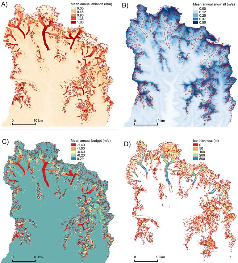
1106                                                                              J. M. Shea et al.: Everest region glacier change

Figure 1. (a) Dudh Koshi basin, eastern Nepal, with current glacier extents in blue (ICIMOD, 2011), EVK2CNR stations (red), GPR profile
sites (yellow). Extents of glacierized (blue) and non-glacierized (orange) regions used for model calibration are also shown. Coordinate
system is UTM 45N. Inset map (b) shows the Dudh Koshi basin in relation to the APHRODITE subset (shaded), and the locations of places
named in the text (A – Annapurna, L – Langtang, K – Kathmandu). Panels (c) and (d) give the location of the transverse GPR surveys (thick
red lines) at Changri Nup and Mera glaciers, respectively.

atures ranging between −25 and +10 ◦ C. During the mon-                1.2   Himalayan glaciology
soon period (June–September), temperatures at 5000 m are
greater than 0 ◦ C and variability is low. The majority of an-         The current status of glaciers varies across the Hindu Kush
nual precipitation (approximately 77 %, derived from grid-             Himalayan (HKH) region. Most areas have seen pronounced
ded climate fields, see below) falls between 1 June and                glacier retreat and downwasting in recent years (Bolch et al.,
30 September during the summer monsoon (Wagnon et al.,                 2012; Kääb et al., 2012; Yao et al., 2012), though some
2013). An additional 14 % of precipitation occurs during the           areas, such as the Karakoram and Pamir ranges, have ex-
pre-monsoon period (March–May), with little or no precipi-             perienced equilibrium or even slight mass gain (Gardelle
tation during the post-monsoon and winter seasons. The in-             et al., 2012, 2013; Jacob et al., 2012). In the Everest region
teraction between moisture advected from the Indian Ocean              (Fig. 1), Gardelle et al. (2013) find an average annual rate
during the monsoon and the two-step topography of the Dudh             of mass loss of −0.26 ± 0.13 m w.e. yr−1 between 2000 and
Koshi region (foothills, main ranges) results in two spatial           2011, while Nuimura et al. (2012) estimate mass loss rates of
maxima of precipitation (Bookhagen and Burbank, 2006).                 −0.40 ± 0.25 m w.e. yr−1 between 1992 and 2008. Between
                                                                       2003 and 2009, thinning rates of −0.40 m yr−1 were esti-
                                                                       mated from ICEsat data (Gardner et al., 2013), which is sim-
                                                                       ilar to the 1962–2002 average thinning rate of −0.33 m yr−1

The Cryosphere, 9, 1105–1128, 2015                                                           www.the-cryosphere.net/9/1105/2015/
J. M. Shea et al.: Everest region glacier change                                                                                       1107

                        7800                                             Table 1. EVK2CNR meteorological stations used to validate down-
                                               Clean ice
                                                                         scaled APHRODITE temperature and precipitation fields.
                        7600                   Debris-covered ice
                        7400
                                                                               Site       Latitude (◦ )   Longitude (◦ )   Elevation (m)
                        7200
                        7000                                                   Lukla       27.69556         86.72306           2660
                        6800                                                   Namche      27.80239         86.71456           3570
                        6600                                                   Pheriche    27.89536         86.81875           4260
                                                                               Pyramid     27.95903         86.81322           5035
                        6400
                        6200
        Elevation (m)

                        6000
                        5800                                             cally extend to lower elevations, and are thus more sensitive
                        5600                                             to temperature changes than those in dry climates (Oerle-
                                                                         mans and Fortuin, 1992). Himalayan glaciers, and glaciers
                        5400
                                                                         of the Dudh Koshi in particular, present a unique chal-
                        5200
                                                                         lenge as observations of temperature and precipitation at high
                        5000
                                                                         elevations are scarce. Regionally, the climate varies from
                        4800                                             monsoon-dominated southern slopes to relatively dry lee-
                        4600                                             ward high-elevation regions. Accordingly, equilibrium line
                        4400                                             altitudes (ELAs) in the region vary both spatially and tempo-
                        4200                                             rally but generally range from 5200 m in the south to 5800 m
                        4000                                             in northern portions of the basin (Williams, 1983; Asahi,
                               0   10 20    30 40 50 60             70   2010; Wagnon et al., 2013). Nearly 80 % of the glacierized
                                           Area (km2 )                   area in the Dudh Koshi basin lies between 5000 and 6000 m
                                                                         (Fig. 2), and the region is expected to be sensitive to climatic
Figure 2. Area of clean and debris-covered glaciers by elevation,
Dudh Koshi basin, Nepal. Extracted from SRTM 90 m DEM and
                                                                         changes.
glacier inventory from ICIMOD (2011)
                                                                         1.3    Historical and projected climate trends

                                                                         Analyses of climate trends in the region are limited, pri-
calculated for glaciers in the Khumbu region (Bolch et al.,              marily due to the lack of long-term records (Shrestha and
2008a, b). Areal extents of glaciers in Sagarmatha National              Aryal, 2011). Available studies indicate that the mean an-
Park decreased 5 % during the second half of the 20th cen-               nual temperatures have increased in the region, and partic-
tury (Bolch et al., 2008b; Salerno et al., 2008; Thakuri et al.,         ularly at high elevations (Shrestha et al., 1999; Rangwala
2014). These estimates do not distinguish between debris-                et al., 2009; Ohmura, 2012; Rangwala and Miller, 2012). Re-
covered and clean-ice glaciers.                                          ported mean annual temperature trends range between 0.025
   One consequence of glacier retreat in the Himalayas is                and 0.06 ◦ C yr−1 for the periods 1971 to 2009 and 1977
the formation of proglacial lakes, which may pose a risk                 to 1994, respectively (Shrestha and Aryal, 2011; Qi et al.,
to downstream communities. Terminus retreat at Lumding                   2013). Changes in temperature are particularly important for
and Imja glaciers, measured at −42 and −34 m yr−1 , re-                  monsoon-type glaciers, which are sensitive to the elevation
spectively, between 1976 and 2000 increased to −74 m yr−1                of the rain/snow threshold during the monsoon season (Bolch
at both glaciers between 2000 and 2007 (Bajracharya and                  et al., 2012). Results from the CMIP5 (Climate Modelling In-
Mool, 2010). Rapid terminus retreat results in the growth of             tercomparison Project) ensemble suggest that temperatures
proglacial lakes which are dammed by lateral and terminal                in the region will increase between 1.3 and 2.4 ◦ C over the
moraines (Bolch et al., 2008b; Benn et al., 2012; Thomp-                 period 1961–1990 to 2021–2050 (Lutz et al., 2013), which
son et al., 2012). The failure of moraine dams in the Koshi              correspond to rates of 0.021 to 0.040 ◦ C yr−1 .
River basin has led to 15 recorded glacier lake outburst flood              Precipitation amounts, timing, and phase will affect
(GLOF) events since 1965, with flows up to 100 times greater             glacier responses on both annual and decadal timescales. In
than average annual flow (Chen et al., 2013), and the fre-               the greater Himalayas, trends in precipitation totals appear
quency of GLOFs in the Himalayas is believed to have in-                 to be mixed and relatively weak (Mirza et al., 1998; Gau-
creased since the 1940s (Richardson and Reynolds, 2000).                 tam et al., 2010; Dimri and Dash, 2012; Qi et al., 2013),
Changes in glacier extents and volumes in response to cli-               though the observational network is composed mostly of
mate change thus have important impacts not only on water                low-elevation valley stations that may not reflect changes in
resources availability but also on geophysical hazards.                  snowfall amounts at higher elevations. General circulation
   The climate sensitivity of a glacier depends primarily on             model projections suggest both increased monsoon precip-
its mass balance amplitude. Glaciers in wetter climates typi-            itation (Kripalani et al., 2007) and delayed monsoon onset

www.the-cryosphere.net/9/1105/2015/                                                               The Cryosphere, 9, 1105–1128, 2015
1108 J. M. Shea et al.: Everest region glacier change
Figure 3. (a) Vertical temperature gradients (γT ) by day of year (DOY) for all years (black) calculated from APHRODITE (1961–2007)
temperature fields and resampled SRTM data, with period mean in grey, (b) daily standard deviation (σ ) of γT , and (c) mean daily coeffi-
cient of determination (R 2 ) calculated from the linear regression of resampled SRTM elevations and APRHODITE cell temperatures. All
temperature/elevation regressions are significant.
(Ashfaq et al., 2009; Mölg et al., 2012) in the 21st century, One- and two-dimensional models of glacier dynamics
while the change in total annual precipitation is mixed. In the have been applied previously to the Khumbu Glacier (Naito
Himalayas, the CMIP5 ensemble shows projected changes et al., 2000) and the East Rongbuk Glacier (Zhang et al.,
in precipitation between −8 to +15 % (Lutz et al., 2013; 2013), respectively. However, these and higher-order mod-
Palazzi et al., 2013). els of glacier dynamics are severely limited by input data
availability (e.g. bed topography, ice temperatures, basal wa-
1.4 Models of glacier change ter pressure) and uncertainties in key model parameters,
and have not been applied at catchment scales in the re-
In spite of the recent observed changes in glaciers in the gion. Debris-covered glaciers, which compose 25 % of to-
Everest region, the reported climatic trends, the expected tal glacierized area, present additional modelling challenges,
glacier sensitivity to climatic change, and the importance of and validation is also limited by the availability of data. Rel-
glacier water resources in the region, few studies have at- atively coarse methods of simulating future glacier change
tempted to model the historical or future response of these (e.g. Stahl et al., 2008) can be improved by applying mod-
glaciers to climate change (Immerzeel et al., 2012, 2013). els that can reasonably simulate key glaciological parameters
Empirical mass balance and snowmelt and ice melt mod- (thickness, velocity, and mass redistribution).
els have been developed from field observations (Ageta and The main objective of this study is to apply a glacier
Higuchi, 1984; Ageta and Kadota, 1992; Nakawo et al., mass balance and redistribution model to the Dudh Koshi
1999) and reanalysis products (Fujita and Nuimura, 2011; River basin, Nepal. To accomplish this, we (1) develop down-
Rasmussen, 2013), and such approaches have been used to scaling routines for temperature and precipitation; (2) cali-
quantify glacier contributions to streamflow (Racoviteanu brate and test the model with available field and remotely
et al., 2013; Nepal et al., 2013). Projections of higher ELAs sensed observations; and (3) explore the modelled sensitiv-
in the region (Fujita and Nuimura, 2011) and volume area- ity of glaciers in the Everest region to future climate change
scaling approaches (Shi and Liu, 2000; Cogley, 2011) indi- with a suite of temperature and precipitation changes from
cate continued mass wastage in the future, yet impact studies the CMIP5 ensemble.
on the response of glaciers to climate change require mod-
els that link mass balance processes with representations of
glacier dynamics.
The Cryosphere, 9, 1105–1128, 2015 www.the-cryosphere.net/9/1105/2015/J. M. Shea et al.: Everest region glacier change 1109
2.1.1 Temperature
8
Downscaled temperature fields at daily 90 m resolution are
Temperature bias (°C)
6 computed as
TZ = γT Z + T0 − CDOY , (1)
4 where γT is the daily vertical temperature gradient (Fig. 3)
Lukla
Namche derived from the 0.25◦ APRHODITE temperatures and
2 Pheriche SRTM elevations, T0 is the daily temperature intercept, and
Pyramid CDOY is a bias correction based on the day of year (Fig. 4).
0 Mean The bias-correction factor is computed from the mean
smoothed daily temperature difference between observed and estimated
mean daily temperatures at four stations operated by the
50 100 150 200 250 300 350 Italian Everest-K2-National Research Centre (EVK2CNR;
Day of year Fig. 1, Table 1), and it ranges from 3 to 6 ◦ C. The EVK2CNR
stations are independent of the APHRODITE product.
Figure 4. Average daily temperature bias (estimated – observed)
for four EVK2CNR sites (2003–2007), their arithmetic mean, and a 2.1.2 Precipitation
smoothed function used as a daily bias correction.
To calculate high-resolution daily precipitation fields from
the APHRODITE subset, we prescribe daily precipitation–
2 Data and methods elevation functions from the 0.25◦ APHRODITE precipita-
tion fields and resampled SRTM data. For each day, we cal-
2.1 Daily climate fields
culate the mean precipitation in 500 m elevation bins (P 500 )
There are few observations of temperature and precipitation and prescribe a fitted linear interpolation function to estimate
in the basin, and no temperature records longer than 15 years precipitation on the 90 m SRTM DEM (Fig. 5).
are available. To generate high-resolution fields of tempera- As APHRODITE fields are based on interpolated station
ture (T ) and precipitation (P ) as inputs to the model, we use data (Yatagai et al., 2012), there is a large uncertainty in
data from the APHRODITE (Asian Precipitation – Highly- the precipitation at high elevations. Independent tests of the
Resolved Observational Data Integration Towards Evalua- precipitation downscaling approach were conducted by com-
tion of Water Resources) project (Yatagai et al., 2009, 2012). paring precipitation observations from the EVK2CNR sta-
APHRODITE products have been previously used to test re- tions with precipitation estimated using the station eleva-
gional climate model simulations in northern India (Math- tion and the daily precipitation–elevation functions (Fig. 6).
ison et al., 2013) and the western Himalaya (Dimri et al., As EVK2CNR stations are not capable of measuring solid
2013), and to compare precipitation data sets in the Hi- precipitation (Wagnon et al., 2013), we only examine days
malayan region (Palazzi et al., 2013). For this study, we use where only liquid precipitation (T > 0) is expected.
APHRODITE T fields (V1204R1) that are based on daily While orographic forcing of moist air masses typically
station anomalies from climatological means, interpolated on produces increased precipitation with elevation, in very high-
0.05◦ grids and then resampled to 0.25◦ fields, and we refer elevation regions (i.e. those greater than 4000 m) both ob-
to Yatagai et al. (2012) for more details. The APHRODITE P servations and models indicate that precipitation totals will
fields (V1101) are based on a similar technique using precip- decrease above a certain elevation (Harper and Humphrey,
itation ratios but incorporate a weighted interpolation scheme 2003; Mölg et al., 2009). This is due in part to the drying ef-
based on topographical considerations (Yatagai et al., 2012). fect from upwind orographic forcing but is also related to the
To generate high-resolution fields of T and P for the low column-averaged water vapour content indicated by the
glacier mass balance model, we extract a 196 (14 × 14) grid Clausius–Clapeyron relation. Given that there are no precipi-
cell subset of the daily APHRODITE T and P fields that tation observations at elevations above 5300 m, and available
covers the Koshi basin (Fig. 1). Approximate elevations for evidence suggests that precipitation will likely decrease at
each 0.25◦ grid cell are extracted from a resampled gap-filled high elevations, we scale estimated precipitation using a cor-
Shuttle Radar Topography Mission (SRTM V4; Farr et al., rection factor pcor :
2007) digital elevation model (DEM). Based on this subset P (Z), Z < Zc
we derive relations between elevation and temperature and P (Z) = P (Z)pcor , Zc ≤ Z < Zm (2)
precipitation respectively at coarse resolution. We then use 0, Z ≥ Zm ,
these relations in combination with the 90 m SRTM DEM to where pcor decreases from 1 at the height of a calibrated
produce high-resolution daily climate fields. threshold elevation (Zc ; Table 2) to 0 at Zm , set here to
7500 m:
www.the-cryosphere.net/9/1105/2015/ The Cryosphere, 9, 1105–1128, 20151110 J. M. Shea et al.: Everest region glacier change
10 25
A) pre-monsoon B) monsoon
Daily precipitation (mm)
Daily precipitation (mm)
8 20
6 15
4 10
2 5
0 0
0 1500 3000 4500 6000 0 1500 3000 4500 6000
10 Elevation (m) 10 Elevation (m)
C) post-monsoon Median D) winter
10th and 90th
Daily precipitation (mm)
Daily precipitation (mm)
8 8
6 6
4 4
2 2
0 0
0 1500 3000 4500 6000 0 1500 3000 4500 6000
Elevation (m) Elevation (m)
Figure 5. APHRODITE precipitation (1961–2007) binned by elevation for pre-monsoon (a), monsoon (b), post-monsoon (c), and winter
(d). Median, 10th percentile, and 90th percentile of daily precipitation are shown. Note different scale for panel (b).
dependence of ddf (Immerzeel et al., 2012). Initial values
pcor = 1 − (Z − Zc )/(Zm − Zc ). (3) for melt factors for snow, ice, and debris-covered glaciers
(Azam et al., 2014) are given in Table 2. The extent of debris-
Above 7500 m, we assume that precipitation amounts mi-
covered glaciers was extracted from the ICIMOD (2011)
nus wind erosion and sublimation (Wagnon et al., 2013) are
glacier inventory.
likely to be negligible. The total area above 7500 m repre-
To redistribute mass from accumulation to ablation ar-
sents only 1.2 % of the total basin area.
eas, we use a simplified flow model which assumes that
2.2 Glacier mass balance and redistribution basal sliding is the principal process for glacier movement
and neglects deformational flow. While cold-based glaciers
Following the methods of Immerzeel et al. (2012) and Im- have been observed on the Tibetan Plateau (Liu et al., 2009),
merzeel et al. (2013), daily accumulation and ablation be- warm-based glaciers and polythermal regimes have been
tween 1961 and 2007 are estimated from the gridded T and identified on the monsoon-influenced southern slopes of the
P fields. All calculations are based on the 90 m SRTM DEM. Himalayas (Mae et al., 1975; Ageta and Higuchi, 1984;
Daily accumulation is equal to the total precipitation when Kääb, 2005; Hewitt, 2007). Our assumption in this case is
T < 0 ◦ C, which is a conservative threshold with respect to a necessary simplification of the sliding and deformational
other studies that have used values of 1.5 or 2 ◦ C (Oerlemans components of ice flow, which have not yet been modelled at
and Fortuin, 1992), but this value has been used in previous the basin scale in the Himalayas.
Himalayan models (Immerzeel et al., 2012). Daily ablation Glacier motion is modelled as slow, viscous flow using
is estimated using a modified degree-day factor (ddfM ) that Weertman’s sliding law (Weertman, 1957), which describes
varies with DEM-derived aspect (θ ) and surface type: glacier movement as a combination of both pressure melting
and ice creep near the glacier bed. Glacier flow is assumed to
ddfM = ddf 1 − Rexp cos θ , (4) be proportional to the basal shear stress (τb , Pa):
2
where ddf is the initial melt factor (in mm ◦ C−1 d−1 ), and τb ≈ v 2 Ru n+1 . (5)
Rexp is a factor which quantifies the aspect (or exposure)
The Cryosphere, 9, 1105–1128, 2015 www.the-cryosphere.net/9/1105/2015/J. M. Shea et al.: Everest region glacier change 1111
6000 5000
Acc. predicted precipitation (mm)
Acc. predicted precipitation (mm)
A) Lukla, 2004 - 2007 B) Namche, 2003 - 2007
5000 4000
4000
3000
3000
2000
2000
1000 1000
0 0
0 1000 2000 3000 4000 5000 6000 0 1000 2000 3000 4000 5000
Acc. observed precipitation (mm) Acc. observed precipitation (mm)
7000 2000
Acc. predicted precipitation (mm)
Acc. predicted precipitation (mm)
6000 C) Pheriche, 2003 - 2007 D) Pyramid, 2003 - 2007
5000 1500
4000
1000
3000
2000 500
1000
0 0
0 1000200030004000500060007000 0 500 1000 1500 2000
Acc. observed precipitation (mm) Acc. observed precipitation (mm)
Figure 6. Accumulated observed and predicted precipitation at the EVK2CNR sites. Days where T < 0 or precipitation observations were
missing were excluded from the analyses.
Table 2. Fixed and calibrated model parameters, with initial values, range, and final calibrated values. Degree-day factors (ddf) varied within
1 standard deviation (SD) (Supplementary Information of Immerzeel et al., 2010).
Initial Calibrated
Parameter Description Units value Range value
ρ Ice density kg m−3 916.7 – –
g Gravitational acceleration m s−2 9.81 – –
τ0 Equilibrium shear stress N m−2 80 000 – –
ν Bedrock roughness unitless 0.1 – –
TS Snow/rain limit ◦C 0 – –
γT Daily vertical temperature gradient ◦ C m−1 variable – –
CDOY Temperature bias correction ◦C variable – –
Rexp Aspect dependence of ddf unitless 0.2 – –
βTH Threshold avalanching angle ◦ 50 – –
R Material roughness coefficient N m−2 s1/3 1.80 × 10⁹ ±5.00 × 10⁸ 1.51 × 10⁸
ddfC Clean ice melt factor mm ◦ C−1 d−1 8.63 ±1 SD 9.7
ddfD Debris-covered ice melt factor mm ◦ C−1 d−1 3.34 ±1 SD 4.6
ddfK Khumbu Glacier melt factor mm ◦ C−1 d−1 6.7 8.6
ddfS Snowmelt factor mm ◦ C−1 d−1 5.3 ±1 SD 5.4
ZC Height of precipitation maximum m a.s.l. 6000 ±500 6268
www.the-cryosphere.net/9/1105/2015/ The Cryosphere, 9, 1105–1128, 20151112 J. M. Shea et al.: Everest region glacier change
70
60
Slope of glacierized cells ( ◦ )
50
40
30
20
10
0
4400 4800 5200 5600 6000 6400 6800 7200 7600 8000 8400
Elevation (m)
Figure 7. Boxplots of the slope of glacierized pixels in the Dudh Koshi basin, grouped by 100 m elevation bands. The boundaries of each
box indicate the upper and lower quartiles, while the middle line of the box shows the median value. Whisker ends indicate the maximum
(minimum) values excluding outliers, which are defined as more (less) than 3/2 times the upper (lower) quartile. Slope values were extracted
from the SRTM 90 m DEM and glacier inventory from ICIMOD (2011).
Here, v (unitless) is a measure of bedrock roughness, R and Schulz, 2010). The approach assumes that all snow in
(Pa m−2 s) is a material roughness coefficient, u is the slid- a given cell is transported to the downstream cell with the
ing speed (m s−1 ) and n (unitless) is the creep constant of steepest slope whenever snow-holding depth and a minimum
Glen’s flow law, here assumed to equal 3 (Glen, 1955). The slope angle is exceeded. The snow-holding depth is deep in
roughness of the bedrock (v) is defined as the dimension of flat areas and shallow in steep areas and decreases exponen-
objects on the bedrock divided by the distance between them. tially with increasing slope angle.
Smaller values for v indicate more effective regelation. R Based on field observations and an analysis of the slopes
is a material roughness coefficient that controls the viscous of glacierized pixels in the catchment (Fig. 7), we assign
shearing (Fowler, 2010). Basal shear stress (τb ) is defined as a threshold avalanching angle (βTH ) of 50◦ . Change in ice
thickness at each time step is thus the net result of ice flow
τb = ρgH sin β, (6) through the cell, ablation, and accumulation from both pre-
cipitation and avalanching. Changes in glacier area and vol-
where ρ is ice density (kg m−3 ), g is gravitational ac-
ume are calculated at daily time steps, and pixels with a
celeration (m s−2 ), H is ice thickness (m), and β is sur-
snow water equivalent greater than 0.2 m w.e. are classified
face slope (◦ ). We assume that motion occurs only when
as glacier. The model does not assume steady-state condi-
basal shear stress exceeds the equilibrium shear stress (τ0 =
tions, and reported changes in volume and area thus represent
80 000 N m−2 ; Immerzeel et al., 2012), and combine Eqs. (5)
transient states within the model.
and (6) to derive the glacier velocity:
2 max(0, τb − τ0 ) 2.3 Model initialization
u n+1 = . (7)
v2R Initial ice thickness for each glacierized grid cell is derived
For each time step, glacier movement in each cell is thus from Eq. (6):
modelled as a function of slope, ice thickness, and assumed τ0
bedrock roughness. The total outgoing ice flux at each time H= , (8)
ρg sin β
step is then determined by the glacier velocity, the horizontal
resolution, and the estimated ice depth. Ice transported out of with a minimum prescribed slope of 1.5◦ . We use τ0 here,
a specific cell is distributed to all neighbouring downstream as the actual basal shear stress depends on the ice thick-
cells based on slope, with steeper cells receiving a greater ness. In the Dudh Koshi basin, Eq. (8) produces a total es-
share of the ice flux. timated glacier volume of 32.9 km3 , based on the ICIMOD
As avalanches can contribute significantly to glacier accu- (2011) glacier inventory and SRTM DEM. While volume–
mulation in steep mountainous terrain (Inoue, 1977; Scherler area scaling relations are uncertain (Frey et al., 2013), empir-
et al., 2011b), the model incorporates an avalanching com- ical relations from Huss and Farinotti (2012) and Radić and
ponent which redistributes accumulated snowfall (Bernhardt Hock (2010) applied to individual glaciers generate basin-
The Cryosphere, 9, 1105–1128, 2015 www.the-cryosphere.net/9/1105/2015/J. M. Shea et al.: Everest region glacier change 1113
wide volume estimates of 31.9 and 27.5 km3 , respectively, The glacier extent score denotes the relative deviation
which lends some support to the approach used here. from a perfect match of the four large glacier termini at the
From the initial ice thicknesses we estimate glacier thick- end of the calibration period (Fig. 1). There are eight test
nesses and extents in 1961 by driving the glacier mass bal- polygons in total that include ice-covered and adjacent ice-
ance and redistribution model with modified APHRODITE free areas. For example, if only 20 % of the glacier polygons
temperature fields. To simulate the observed climate in the in Fig. 1 are ice covered then the score equals 0.8. The mass
region prior to 1961, temperatures in the initialization run balance score is based on the relative offset from the catch-
are decreased by −0.025 ◦ C yr−1 (Shrestha and Aryal, 2011), ment mean mass balance of −0.40 m w.e. yr−1 over the pe-
for a total decrease of −1.2 ◦ C over the 47-year initialization riod 1992–2008:
period. Precipitation is left unchanged in the model initial-
ization, and we use uncalibrated model parameters (Table 2). SMB = |(Bm / − 0.4) − 1|. (9)
Mass change at the end of the 47-year initialization pe-
If the modelled mean mass balance (Bm ) equals
riod is close to zero, indicating that near-equilibrium con-
−0.20 m w.e. yr−1 , then the mass balance score (SMB )
ditions have been realized. Additional runs of the initializa-
is 0.5. The total ice area score is based on the departure
tion period, with temperatures fixed at −1.2 ◦ C, yield rela-
from the total glacierized area at the end of the simulation
tively small changes in glacier thickness (Fig. 8). However,
(410 km2 , ICIMOD, 2011). If the simulated ice extent is
it is possible that there are significant uncertainties in our es-
300 km2 , then the score is 0.27 ((410–300)/410). Finally the
timates of initial (1961) thicknesses and extents, given the
flow velocity score quantifies the deviation from a mean
forcings and parameter set used, and the lag in glacier geom-
glacier velocity of debris-covered tongues from 1992 to
etry responses to climate forcings.
2008 (10 m yr−1 ). For example, if the average simulated
2.4 Model calibration flow velocity is 2 m yr−1 , then the score is 0.8. The final
score used to select the optimal parameter set is a simple
From the modelled 1961 ice thicknesses and extents, the addition of the four scores.
model is calibrated with six parameters: degree-day factors
for clean ice (ddfC ), debris-covered ice (ddfI ), snow (ddfS ), 2.5 Model validation
and debris covered ice on the Khumbu Glacier (ddfK ), ma-
Temperature and precipitation fields developed for this study
terial roughness coefficient R, and elevation of the precip-
were tested independently using point observations of mean
itation maximum ZC (Table 2). Initial simulations showed
daily temperature and total daily precipitation at the four
anomalous flow velocities of the Khumbu Glacier, which
EVK2NCR sites. We calculate mean bias error (MBE) and
may be due to the assumption that basal sliding is the main
root mean square error (RMSE) to evaluate the skill of the
process of movement. This may not hold given the steep ice-
elevation-based downscaling.
fall above the glacier tongue and the large high-altitude ac-
To validate the calibrated glacier mass balance and redis-
cumulation area. We have corrected for this by calibrating a
tribution model, model outputs are compared against the fol-
specific melt factor for this glacier, though improved repre-
lowing independent data sets:
sentation of the glacier dynamics should reduce the need for
a separate ddfK . Twenty parameter sets (Table 3) were devel- – ice thickness profiles derived from ground-penetrating
oped by varying the six calibration factors within specified radar (GPR) at Mera Glacier (Wagnon et al., 2013) and
ranges (Table 2). Initial values for each parameter were se- Changri Nup Glacier (Vincent, unpublished data);
lected from published studies.
For each of the 20 runs (Table 4), we quantify the model – annual mass balance and glacier mass balance gradients
skill by scoring (a) modelled and observed glacier extents calculated from surface observations at Mera Glacier
at the termini of four large glaciers in the catchment (ICI- (Wagnon et al., 2013);
MOD, 2011), (b) the geodetically derived mean basin-wide
– decadal glacier extents (1990, 2000, 2010) extracted
glacier mass balance of −0.40 m w.e. yr−1 over the period
from Landsat imagery (Bajracharya et al., 2014b);
1992–2008 (Nuimura et al., 2012), (c) a mean velocity of
10 m yr−1 for debris-covered glaciers (Nakawo et al., 1999; – basin-wide mean annual mass balance from 2000 to
Quincey et al., 2009), and (d) the total glacierized area in 2011 (Gardelle et al., 2013), and from 1970 to 2007
2007 (410 km2 ; ICIMOD, 2011). These tests gauge the abil- (Bolch et al., 2011).
ity of the model to accurately reproduce key glacier param-
eters: extent, mass change, and velocity. Scores are derived
2.6 Glacier sensitivity to future climate change
from the difference between modelled and observed quanti-
ties, with a score of zero indicating a perfect match. Scores To examine the sensitivity of modelled glaciers to future cli-
for all four metrics are added to obtain an overall ranking of mate change, we drive the calibrated model with temperature
the 20 parameter sets and are weighted equally. and precipitation anomalies prescribed from eight CMIP5
www.the-cryosphere.net/9/1105/2015/ The Cryosphere, 9, 1105–1128, 20151114 J. M. Shea et al.: Everest region glacier change
100 6000
A B
80
5000
60
40 4000
20
Count
3000
0
−20 2000
−40
1000
−60
−80 0
−150 −100 −50 0 50 100 150
−100 Thickness difference (m)
Figure 8. (a) Differences in modelled ice thickness (in m) between the end of the first initialization run (47 years) and after an additional
94 years of simulation with dT = −1.2 ◦ C. (b) Histogram of differences in modelled ice thickness.
Table 3. Parameter sets used in the calibration procedure. Degree-day factors (ddfn ) are given in units of mm ◦ C−1 d−1 , R is unitless, and
ZC is in m. Mean (x) and standard deviation (σ ) are given at the bottom of the table.
Run ddfC ddfD ddfK ddfS R ZC
1 10.1 2.4 5.7 5.1 965538934 5948
2 9.8 3.7 6.8 4.6 862185519 5974
3 9.2 4.1 8.5 3.6 1326340408 5544
4 8.8 1.7 5.3 5.7 2115148902 6392
5 9.7 4.6 8.6 5.4 1507211339 6268
6 8.9 1.9 6.8 4.3 1757035837 5712
7 9.3 3.6 7.3 6.6 1602852068 5810
8 8.9 2 7 5.3 1891517886 7175
9 9.3 2.9 8.2 5.7 965461867 6663
10 8.1 3.1 9 5.8 1966902971 6339
11 9.3 4.1 7 5.1 2119160369 5804
12 10.1 3.3 6.4 4.7 1183544033 5774
13 10.2 2.2 5.7 5.1 2027971886 5960
14 9.3 5.2 6.6 6.4 1642592045 5887
15 8.5 3.2 6.7 3.9 1674708607 5466
16 8.1 4.3 4.2 5.5 1278943171 6877
17 10.2 3.5 5.4 5.6 1687134148 6314
18 10.7 2 6.2 5.3 1920883676 6270
19 7.6 2.9 7.2 4.6 2402645369 5586
20 10.8 3.5 6 6.4 1885850339 5673
x 9.3 3.2 6.7 5.2 1639181469 6072
σ 0.87 0.98 1.23 0.8 428282810 459
climate simulations that represent cold/warm and dry/wet climate change are examined through the mean and standard
end-members (Table 5; Immerzeel et al., 2013). Decadal T deviation of modelled ice areas and volumes derived from the
and P anomalies relative to 1961–1990 are extracted from eight CMIP5 models. As the model is empirically based and
the CMIP5 end-members. Temperature trends are strong in we assume only changes in T and P (all other state and in-
all CMIP5 simulations, with ensemble mean temperature in- put variables remain unchanged), we stress that the resulting
creases to 2100 as great as +8 ◦ C in late winter and early glacier change realizations are a reflection of the modelled
spring (January–April). Precipitation anomalies do not show sensitivity to climate change, as opposed to physically based
any significant trends and vary between 0.4 and 1.8 times projections.
the baseline period. Uncertainties in our scenarios of future
The Cryosphere, 9, 1105–1128, 2015 www.the-cryosphere.net/9/1105/2015/J. M. Shea et al.: Everest region glacier change 1115
Table 4. Scores (unitless) from the 20 calibration runs versus independent calibration data. Calibration targets were observed extents of four
large termini, basin-wide net mass balance of −0.40 m (Nuimura et al., 2012), total glacier area of 410 km2 in 2010 (ICIMOD, 2011), and
mean velocity of 10 m yr−1 on debris-covered tongues (Quincey et al., 2009). Mean and standard deviation (σ ) of scores are provided at the
bottom of the table, and scores for the selected run are in bold.
Run Terminus extents Ba Total area Velocity Total score
1 0.20 0.46 0.04 3.44 4.14
2 0.19 0.31 0.03 2.78 3.31
3 0.19 0.26 0.01 0.34 0.79
4 0.19 0.69 0.04 0.38 1.30
5 0.17 0.19 0.06 0.05 0.47
6 0.20 0.58 0.01 0.75 1.54
7 0.18 0.23 0.09 0.10 0.59
8 0.19 0.70 0.03 0.88 1.80
9 0.20 0.46 0.05 3.13 3.83
10 0.18 0.45 0.05 0.01 0.69
11 0.18 0.24 0.05 0.47 0.94
12 0.19 0.33 0.04 1.21 1.76
13 0.19 0.52 0.04 0.08 0.84
14 0.17 0.05 0.09 0.44 0.75
15 0.19 0.39 0.00 0.08 0.65
16 0.18 0.44 0.04 0.72 1.37
17 0.18 0.36 0.06 0.02 0.63
18 0.19 0.56 0.05 0.37 1.18
19 0.19 0.46 0.02 0.36 1.03
20 0.18 0.20 0.10 0.37 0.85
x 0.19 0.39 0.04 0.80 1.42
σ 0.01 0.18 0.03 0.87 0.90
Table 5. Projected mean annual temperature and precipitation changes from 1961–1990 to 2021–2050, extracted from RCP4.5 and RCP8.5
CMIP5 runs. See Supplementary Information from Immerzeel et al. (2013) for more information.
Scenario Description dP (%) dT (◦ C) Model Ensemble
RCP4.5 Dry, Cold −3.2 1.5 HADGEM2-CC r1i1p1
RCP4.5 Dry, Warm −2.3 2.4 MIROC-ESM r1i1p1
RCP4.5 Wet, Cold 12.4 1.3 MRI-CGCM3 r1i1p1
RCP4.5 Wet, Warm 12.1 2.4 IPSL-CM5A-LR r3i1p1
RCP8.5 Dry, Cold −3.6 1.7 HADGEM2-CC r1i1p1
RCP8.5 Dry, Warm −2.8 3.1 IPSL-CM5A-LR r2i1p1
RCP8.5 Wet, Cold 15.6 1.8 CSIRO-MK3-60 r1i1p1
RCP8.5 Wet, Warm 16.4 2.9 CAN-ESM2 r2i1p1
3 Results sults in a less negative moist adiabatic lapse rate. These find-
ings are consistent with temperature gradient observations
3.1 APHRODITE downscaling between −0.0046 ◦ C m−1 (monsoon) and −0.0064 ◦ C m−1
(pre-monsoon) in a nearby Himalayan catchment (Immerzeel
et al., 2014b). The standard deviation in calculated γT is low-
Daily vertical temperature gradients calculated from the est during the monsoon and greatest in the winter.
APHRODITE temperature fields and resampled SRTM range At all four EVK2CNR stations, daily temperatures esti-
from −0.010 to −0.004 ◦ C m−1 and are highly significant mated from APHRODITE vertical gradients are greater than
(Fig. 3). Calculated γT values are most negative in the pre- observed, with mean daily differences ranging from −1 to
monsoon (mid-April) and least negative during the active +8 ◦ C (Fig. 4). Micro-meteorological conditions may con-
phase of the summer monsoon (mid-June to late August). tribute to the larger biases observed at Pyramid (winter)
This is likely a function of the increased moisture advec- and Pheriche (summer). During the summer monsoon pe-
tion in the monsoon and pre-monsoon periods, which re-
www.the-cryosphere.net/9/1105/2015/ The Cryosphere, 9, 1105–1128, 20151116 J. M. Shea et al.: Everest region glacier change riod (mid-June to mid-September), the mean difference for uncertainties are the standard deviation in modelled values all stations is approximately 5 ◦ C. We develop a bias correc- from the 20 simulations. Modelled ice volumes from the 20 tion for the day of year (DOY) based on the mean tempera- calibration runs (Fig. 10) decrease from 41.0 km3 in 1961 to ture bias from the four stations, which ranges from 3.22 to between 31.6 and 37.1 km3 in 2007, with a 20-member mean 6.00 ◦ C. The largest bias coincides with the approximate on- of 34.5 ± 1.5 km3 at the end of the simulation period. The set of the summer monsoon (DOY 150, or 31 May). A pos- ensemble mean modelled glacierized area in the calibration sible mechanism for this is the pre-monsoon increase in hu- runs decreases from 499 km2 to 392 ± 11 km2 , with a final midity at lower elevations, which would be well-represented range of 374 to 397 km2 . in the gridded APHRODITE data but not at the higher eleva- Parameters for the calibrated model were chosen from tion EVK2CNR stations. The increased humidity would re- Run 5, which had the lowest additive score of the 20 pa- sult in a less negative derived temperature gradient, and thus rameter sets (Table 4). Run 5 generates glacier volume and greater errors at the high-elevation stations. The variability area totals that are lower but within 1 standard deviation of in calculated temperature gradients is sharply reduced at on- the model mean (Fig. 10). The selected parameter set con- set of the monsoon, which supports this hypothesis. Bias- tains degree-day factors (Table 2) that are all slightly higher corrected estimates of daily temperature (Fig. 9) have root than those observed by Azam et al. (2014) at Chhota Shi- mean squared errors (RMSE) of 1.21 to 2.07 ◦ C and mean gri Glacier but are similar to values obtained for snow and bias errors (MBE) of −0.87 to 0.63 ◦ C. ice by Singh et al. (2000) at Dokriani Glacier, Garhwal Hi- Based on the calculated daily temperature gradients, in- malaya. The value of the material roughness coefficient in tercepts, and the bias correction, we estimate the height of the selected parameter set lies between the values used pre- the 0 ◦ C isotherm (ZT =0 ) for the period 1961–2007 to exam- viously in Baltoro (Pakistan) and Langtang (Nepal, Fig. 1) ine melt potential and snow-line elevations. Mean monthly catchments (Immerzeel et al., 2013, Supplementary Informa- values of ZT =0 range from 3200 m (January) to 5800 m tion). (July), though it can reach elevations of over 6500 m on Spatially distributed output from the calibrated model occasion. This corresponds to meteorological observations (Run 5), 1961–2007, is summarized in Fig. 11. Mean an- from Langtang Valley, Nepal (Shea et al., 2015), and from nual ablation (Fig. 11a) ranges from 0 to 4.00 m w.e. yr−1 , the Khumbu Valley (http://www.the-cryosphere-discuss.net/ though most modelled values are less than 1.80 m w.e. yr−1 . 7/C1879/2013/tcd-7-C1879-2013.pdf). Debris-covered termini, despite having lower degree-day fac- Daily precipitation–elevation functions (Fig. 5) exhibit tors, are nevertheless subjected to large melt rates due to strong decreases in precipitation above 4000 m, particularly their relatively low elevation and consequently higher tem- in the monsoon and pre-monsoon periods. Absolute precip- peratures. Our model generates maximum melt rates at the itation totals are greatest during the monsoon period, but transition between debris-covered and clean glacier ice, at el- large precipitation events can still occur in the post-monsoon evations of approximately 5000 m (Fig. 2). This is consistent period (October–November). As often observed in high- with geodetic observations of mass change in the catchment elevation environments, daily precipitation totals observed at (e.g. Bolch et al., 2008b). Maximum mean annual snowfall the EVK2CNR stations are not well captured by the down- (Fig. 11b) amounts of up to 0.50 m w.e. yr−1 are observed scaling process (Fig. 6). This is likely due to the difficulties in at 6268 m (the calibrated value of ZC , Table 2), but due to estimating precipitation in complex terrain (Immerzeel et al., the precipitation scaling function (Eq. 2) the highest peaks 2012; Pellicciotti et al., 2012) and to errors in the precipita- receive zero snowfall amounts. The calibrated height of ZC tion measurements. For daily liquid precipitation (T > 0 ◦ C), (6268 m) is similar to the elevation of maximum snowfall RMSEs range between 2.05 and 8.21 mm, while MBEs range (between 6200 and 6300 m) estimated for the Annapurna from −0.85 to 1.77 mm. However, accumulated precipitation range in mid-Nepal (Fig. 1; Harper and Humphrey, 2003). totals (Fig. 6) and mean monthly precipitation values show Modelled glacier velocities during the calibration period greater coherence, which lends some support for the down- are less than 10 m yr −1 over debris-covered glacier termini scaling approach used. At Pyramid (5035 m), the highest sta- and between 30 and 100 m yr−1 between the accumulation tion with precipitation observations, the fit between cumula- and ablation zones. While there are differences in both the tive predicted and observed precipitation is quite close. How- spatial pattern and magnitude of modelled and observed ve- ever, at Pheriche (4260 m), predicted precipitation is nearly locities (e.g. Quincey et al., 2009), we feel that our simpli- double that observed over the period of record, which sug- fication of glacier dynamics is unavoidable in the current gests that further refinements to the precipitation downscal- study, and the development of higher-order physically based ing method are needed. models will lead to improved representations of glacier flow. 3.2 Model results and validation 3.2.1 Mass balance For the calibration runs, we report here volume and area val- Over the entire domain, modelled mean annual mass bal- ues averaged between 1 November and 31 January. Reported ances (ba ; Fig. 11c) range from −4.6 to +3.0 m w.e. yr−1 , The Cryosphere, 9, 1105–1128, 2015 www.the-cryosphere.net/9/1105/2015/
J. M. Shea et al.: Everest region glacier change 1117
Figure 9. Mean daily temperatures observed at EVK2CNR sites (2003–2007) versus bias-corrected temperatures estimated from
APHRODITE temperature fields.
42
Ice volume (km3)
38
34
Mean
Run 5
500 30
Ice area (km2)
450
Date
400
350
1960 1970 1980 1990 2000
Figure 10. Top panel: modelled mean (1 November–31 January) ice volumes
Date from the 20 calibration runs, 1961–2007, with multi-model
mean (black line), minimum and maximum modelled volumes (shaded area), and results from Run 5 (dashed line). Bottom panel: as above
but for modelled glacier areas from the 20 calibration runs.
with the majority of values falling between −1.4 and −0.26 ± 0.13 m w.e. yr−1 given by Gardelle et al. (2013) and
+0.1 m w.e. yr−1 . The spatial patterns of modelled annual −0.27 ± 0.08 m w.e. yr−1 given by Bolch et al. (2011) for the
mass balance are consistent with the geodetic estimates Khumbu region only.
of mass change between 2000 and 2010, and our mod- The overall Dudh Koshi mass balance gradient (Run 5),
elled basin-wide mass balance of −0.33 m w.e. yr−1 is only calculated from median modelled ba for all glacierized cells
slightly more negative than the basin-wide estimates of in 100 m intervals between 4850 and 5650 m, is equiva-
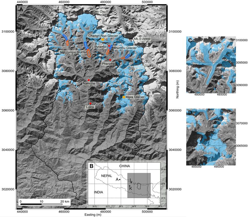
www.the-cryosphere.net/9/1105/2015/ The Cryosphere, 9, 1105–1128, 20151118 J. M. Shea et al.: Everest region glacier change Figure 11. Results from the calibrated model run, 1961–2007. (a) Mean annual ablation, (b) mean annual snowfall, (c) mean annual mass budget, and (d) final ice thickness. Extents of glacierized and non-glacierized calibration regions are shown in (d). lent to 0.27 m w.e. (100 m)−1 (Fig. 12). The range of mass rameter sets. Surface mass balance observations at the balance gradients for the other 19 parameter sets ranges same site from 2007 to 2012 range between −0.67 and from 0.10 to 0.34 m w.e. (100 m)−1 . The mass balance gra- +0.46 m w.e. (Wagnon et al., 2013). As model and ob- dient from Run 5 gives a basin-wide ELA at approximately servation periods do not overlap, direct comparisons be- 5500 m, which agrees with previously published estimates tween modelled and observed mass balances are not pos- (Williams, 1983; Asahi, 2010; Wagnon et al., 2013). Mass sible. However, the mean mass balance observed at Mera balance gradients (Run 5) at Mera and Naulek glaciers are Glacier between 2007 and 2012 is −0.08 m w.e., whereas approximately 0.40 and 0.68 m w.e. (100 m)−1 , respectively, the mean modelled mass balance between 2000 and 2006 is between 5350 and 5600 m. These values compare well with −0.16 m w.e. We note that our reconstructed mass balance the gradients of 0.48 and 0.85 m w.e (100 m)−1 observed over series at Mera Glacier shows strong similarities to the re- the same elevation range at Mera and Naulek between 2007 constructed mass balance at Chhota Shigri Glacier (Azam and 2012 (Wagnon et al., 2013). Calculated mass balance et al., 2014), with balanced conditions in the late 1980s and gradients from the different parameter sets range from 0.31 early 1990s. Standard deviations of observed and modelled to 0.35 m w.e. (100 m)−1 at Mera Glacier and from 0.46 to mass balance are 0.51 and 0.29 m w.e., respectively, and the 0.72 m w.e. (100 m)−1 at Naulek Glacier (Fig. 12). greater variability in observed ba is likely linked to the short Modelled annual mass balances (Ba ) at Mera Glacier observation period (5 years) and to enhanced local variabil- (1961–2007) range between −1.45 and +0.11 m w.e. ity which cannot be captured with downscaled climate fields. (Fig. 13), with low variability amongst the different pa- The mass balance model, although it may underestimate the The Cryosphere, 9, 1105–1128, 2015 www.the-cryosphere.net/9/1105/2015/
J. M. Shea et al.: Everest region glacier change                                                                                                                                                     1119

                                                               3                                                                                                      0.8

                                                               2                                                                                                      0.7

                                                                                                                         Mass balance gradients (m w.e. (100 m)−1 )
                      Modelled mean annual ba (m w.e. yr−1 )
                                                               1                                                                                                      0.6

                                                               0                                                                                                      0.5

                                                               1                                                                                                      0.4

                                                               2                                                                                                      0.3

                                                               3                                                                                                      0.2

                                                               4                                                                                                      0.1

                                                               5                                                                                                      0.0
                                                                   4400 4800 5200 5600 6000 6400 6800 7200 7600                                                             Dudh Mera Naulek
                                                                                   Elevation (m)
Figure 12. Left: boxplots of modelled mean annual mass balance (m w.e. yr−1 ) calculated for 100 m intervals (1961–2007) for the entire
Dudh Koshi basin. Calculated mass balance gradient of 0.27 m w.e. (100 m)−1 between 4850 and 5650 m is shown in red. Right: boxplots
of mass balance gradients calculated for all 20 calibration model runs for the entire Dudh Koshi (between 4850 and 5650 m), Mera Glacier
(between 5350 and 5600 m), and Naulek Glacier (between 5350 and 5600 m). The gradients calculated for Run 5 are shown in red.
                          Net mass balance (m w.e.)

                                                               0.5
                                                               −0.5
                                                               −1.5

                                                                      1962   1967   1972   1977   1982   1987   1992   1997                                             2002    2007   2012

Figure 13. Modelled (dashed) and observed (solid) annual net mass balance at Mera Glacier, 1961–2007. Error bars for the modelled mass
balances derived from the standard deviation of the annual mass balances extracted from 20 calibration runs, and error bars for the observed
mass balances are from Wagnon et al. (2013).

inter-annual variability, is able to simulate a surface mass bal-                                        Camp to less than 100 m near the terminus (Gades et al.,
ance that is in a plausible and realistic range.                                                         2000). Our model accurately captures this decrease in the up-
                                                                                                         per portions but overestimates ice thickness in the relatively
3.2.2   Modelled and observed glacier thickness                                                          flat terminus. Recent observations of ice thickness obtained
                                                                                                         from ground penetrating radar (GPR) surveys in the basin are
At the end of the calibrated run (1961–2007), modelled ice                                               examined in detail below.
thicknesses range between 0 and 620 m, though 98 % of these                                                 Estimates of glacier thickness extracted from the cali-
are less than 205 m (Fig. 11d). Similar ice thicknesses have                                             brated model and are compared with depth profiles found
been estimated for the large debris-covered Gangotri Glacier,                                            with GPR surveys conducted at Mera Glacier (Wagnon et al.,
Indian Himalaya, using slope, surface velocities, and simple                                             2013) and Changri Nup Glacier (C. Vincent, unpublished
flow laws (Gantayat et al., 2014). Due to the model formula-                                             data). To facilitate the comparison, we obtained surface el-
tion, low-angle slopes on glacier termini may result in unre-                                            evations and bedrock depths from the GPR surveys, and we
alistic estimates of ice depth, and a minimum surface slope                                              matched these to the modelled ice thicknesses of the corre-
of 1.5◦ is prescribed in the model. Radio-echo surveys in                                                sponding pixels (Fig. 14). At the lower elevation profile on
1999 indicated that centerline ice thicknesses on the Khumbu                                             Mera Glacier (5350 m), the shape of the bedrock profile is
Glacier decreased from approximately 400 m at Everest Base

www.the-cryosphere.net/9/1105/2015/                                                                                                                                     The Cryosphere, 9, 1105–1128, 2015
1120 J. M. Shea et al.: Everest region glacier change
A) Observed
Glacier area change below 5500 m (% yr−1)
Elevation (m)
Calibration runs
5500
−0.3
Run 5
●
−0.4
5400
●
−0.5
0 200 400 600 800
Horizontal distance (m)
−0.6
●
B)
5400
Elevation (m)
−0.7
5300
●
−0.8
●
5200
0 200 400 600 800
Horizontal distance (m) 1980s 1990s 2000s
C) Figure 15. Rates of historical glacier area change below 5500 m
5550
Elevation (m)
(% yr−1 ) from the 20 model runs. Remotely sensed rates of glacier
area change and Run 5 results are shown as black and grey points,
5450
respectively. The 1980’s inventory contained inaccuracies related to
the resolution of the imagery and the misclassification of snow as
5350
glacier ice, and an observed rate of change from 1980 to 1990 is not
0 100 200 300 400
included here.
Horizontal distance (m)
Figure 14. Glacier depths estimated from transverse ground-based modelled and observed extents we use the mean extent at the
GPR surveys and the mass balance and redistribution model, for (a)
end of the ablation season (1 November–31 January).
profile at 5350 m on Mera Glacier, (b) profile at 5520 m on Mera
Glacier, and (c) profile at Changri Nup Glacier (Fig. 1). Ice depth
Using semi-automated classifications of Landsat imagery,
estimates for all 20 calibration runs are given in grey, and the results glacier extents in the Dudh Koshi basin were constructed for
for Run 5 are shown as a dashed black line. 1990, 2000, and 2010 (ICIMOD, 2011; Bajracharya et al.,
2014a, available at rds.icimod.org). As the glacier change
signal is greatest at lower elevations, and errors in glacier de-
lineation due to persistent snow cover are possible at higher
similar to the model, but ice thicknesses are approximately elevations, we consider the change in glacier area below
half what is observed or less. This may be due in part to the 5500 m, which roughly equals the equilibrium line altitude
surface slope extracted from the DEM, which controls the in the catchment.
modelled ice thickness. The transect at 5350 m was collected Below 5500 m, the observed rate of glacier area change in
in a flat section between two steeper slopes, which would the Dudh Koshi was −0.61 % yr−1 between 1990 and 2000,
likely be mapped as a steep slope in the DEM. For the profile and −0.79 % yr−1 between 2000 and 2010. For the 20 pa-
at 5520 m both the shape and the depths of the bedrock pro- rameter sets, modelled rates of glacier area change below
file are generally well-captured by the model. At the Changri 5500 m (Fig. 15) vary between −0.24 % and 0.41 % yr−1
Nup cross section, which lies on a relatively flat section of the (1990–2000) and −0.54 and −0.85 % yr−1 (2000–2007) for
main glacier body, modelled ice depths are approximately the 20 parameter sets. The calibrated run (Run 5) gives area
two-thirds of the observed. Modelled ice depths do not ap- change rates of −0.36 and −0.75 % yr−1 for the 1990–2000
pear to be highly sensitive to the range of model parameters and 2000–2007 periods, respectively. Both modelled and ob-
used in the 20 calibration runs, though variability is higher served glacier change are of similar magnitudes, and both
for Mera Glacier than for Changri Nup. show a consistent trend of increasing area loss, which is
corroborated by other studies in the region (Bolch et al.,
3.2.3 Modelled and observed glacier extents and 2008b; Thakuri et al., 2014). Salerno et al. (2014) cite a
shrinkage weakened monsoon with reduced accumulation at all eleva-
tions as a main reason for the increased mass loss in recent
Modelled historical changes in glacier area (Fig. 10) ex- years. Differences between modelled and observed rates of
hibit greater variability than modelled ice volumes. This is glacier shrinkage can be attributed to errors in the glacier in-
largely due to the sensitivity of the modelled glacier area ventory, e.g. geometric correction and interpretation errors,
to large snowfall events, as snowfall amounts greater than uncertainty in our estimates of initial ice volumes, and other
the 0.2 m w.e. threshold are classified as glacier. To compare model errors which are discussed below.
The Cryosphere, 9, 1105–1128, 2015 www.the-cryosphere.net/9/1105/2015/You can also read