Quantification of different flow components in a high-altitude glacierized catchment (Dudh Koshi, Himalaya): some cryospheric-related issues
←
→
Page content transcription
If your browser does not render page correctly, please read the page content below
Hydrol. Earth Syst. Sci., 23, 3969–3996, 2019
https://doi.org/10.5194/hess-23-3969-2019
© Author(s) 2019. This work is distributed under
the Creative Commons Attribution 4.0 License.

Quantification of different flow components in a high-altitude
glacierized catchment (Dudh Koshi, Himalaya): some
cryospheric-related issues
Louise Mimeau1 , Michel Esteves1 , Isabella Zin1 , Hans-Werner Jacobi1 , Fanny Brun1 , Patrick Wagnon1 ,
Devesh Koirala2 , and Yves Arnaud1
1 Université Grenoble Alpes, IRD, Grenoble INP, CNRS, IGE, Grenoble, France
2 Nepal   Academy of Science and Technology, NAST, Kathmandu, Nepal

Correspondence: Michel Esteves (michel.esteves@ird.fr)

Received: 25 January 2018 – Discussion started: 9 February 2018
Revised: 20 June 2019 – Accepted: 15 August 2019 – Published: 27 September 2019

Abstract. In a context of climate change and water demand         flow components. In the presented case study, ice melt and
growth, understanding the origin of water flows in the Hi-        snowmelt contribute each more than 40 % to the annual wa-
malayas is a key issue for assessing the current and future       ter inputs and 69 % of the annual stream flow originates
water resource availability and planning the future uses of       from glacierized areas. The analysis of the seasonal contri-
water in downstream regions. Two of the main issues in the        butions highlights that ice melt and snowmelt as well as rain
hydrology of high-altitude glacierized catchments are (i) the     contribute to monsoon flows in similar proportions and that
limited representation of cryospheric processes controlling       winter outflow is mainly controlled by the release from the
the evolution of ice and snow in distributed hydrological         englacial water storage. The choice of a given parametriza-
models and (ii) the difficulty in defining and quantifying the    tion for snow and glacier processes, as well as their relative
hydrological contributions to the river outflow. This study       parameter values, has a significant impact on the simulated
estimates the relative contribution of rainfall, glaciers, and    water balance: for instance, the different tested parameteri-
snowmelt to the Khumbu River streamflow (Upper Dudh               zations led to ice melt contributions ranging from 42 % to
Koshi, Nepal, 146 km2 , 43 % glacierized, elevation range         54 %. The sensitivity of the model to the glacier inventory
from 4260 to 8848 m a.s.l.) as well as the seasonal, daily, and   was also tested, demonstrating that the uncertainty related to
sub-daily variability during the period 2012–2015 by using        the glacierized surface leads to an uncertainty of 20 % for the
the DHSVM-GDM (Distributed Hydrological Soil Vegeta-              simulated ice melt component.
tion Model – Glaciers Dynamics Model) physically based
glacio-hydrological model. The impact of different snow
and glacier parameterizations was tested by modifying the
                                                                  1   Introduction
snow albedo parameterization, adding an avalanche mod-
ule, adding a reduction factor for the melt of debris-covered     The Himalayan mountain range is known for being the water
glaciers, and adding a conceptual englacial storage. The rep-     tower of Central and South Asia (Immerzeel et al., 2010).
resentation of snow, glacier, and hydrological processes was      Its high-elevation glaciers and snow cover play an important
evaluated using three types of data (MODIS satellite images,      role in the regional hydrological system (Kaser et al., 2010;
glacier mass balances, and in situ discharge measurements).       Racoviteanu et al., 2013) and provide water resources for the
The relative flow components were estimated using two dif-        population living in the surrounding countries (Viviroli et al.,
ferent definitions based on the water inputs and contribut-       2007; Singh et al., 2016; Pritchard, 2017).
ing areas. The simulated hydrological contributions differ
not only depending on the used models and implemented
processes, but also on different definitions of the estimated

Published by Copernicus Publications on behalf of the European Geosciences Union.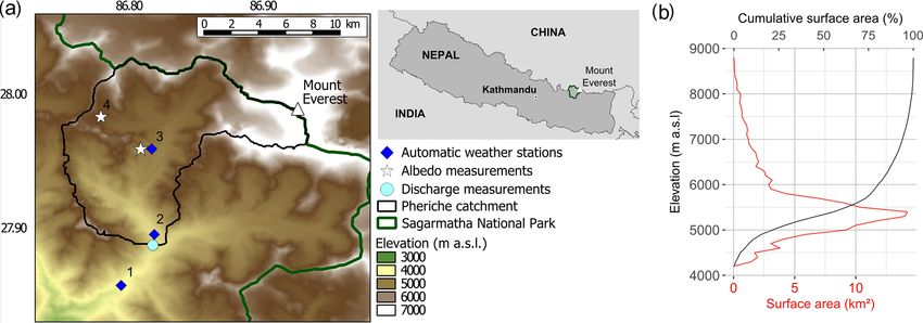
3970                          L. Mimeau et al.: Quantification of different flow components in the Dudh Koshi catchment

   In the Hindu Kush-Himalaya (HKH) region climate                 amount of meltwater generated in glacierized catchments in
change is expected to cause shrinkage of the snow and ice          the Himalayas. Many other cryospheric processes, such as
cover (Bolch et al., 2012; Benn et al., 2012; Kraaijenbrink        the liquid water storage and transfer through glaciers, snow
et al., 2017). Changes in glacier and snow cover runoff are        transport by avalanches or wind, glacial lake dynamics, and
likely to have a significant impact on the hydrological regime     snow albedo evolution are either very simplified or not at all
(Akhtar et al., 2008; Immerzeel et al., 2012; Lutz et al., 2014;   represented by the models (Chen et al., 2017). It is therefore
Nepal, 2016). Development of tourism is also affecting the         important to estimate the impact of such simplified represen-
accessibility to water during the peak of the tourist season.      tations of cryospheric processes on modeling results.
In the Everest region in Nepal water needs have increased             Delineation of the glacierized areas is another key entry
within the past decades due to higher demand in water sup-         element in the glacio-hydrological model. Glacier invento-
ply for tourists and hydroelectricity production, leading to       ries are commonly used as forcing data to delineate glacier-
water shortages during months with low flows (winter and           ized areas in glacio-hydrological modeling studies. There are
spring) (McDowell et al., 2013). Understanding the past and        three global major glacier inventories, i.e., the World Glacier
present hydrological regimes, and more particularly estimat-       Inventory (Cogley, 2009), GlobGlacier (Paul et al., 2009),
ing the seasonal contributions of ice melt, snowmelt, and          and the Randolph Glacier Inventory (Pfeffer et al., 2014), and
rainfall to outflows, is thus a key issue for managing water re-   several regional glacier inventories in the HKH region (ICI-
sources within the next decades. Indeed, the quantification of     MOD, Bajracharya et al., 2010; Racoviteanu et al., 2013),
the ice melt contribution enables us to assess the proportion      showing substantial differences. These can be due to the def-
of water currently available which is coming from a long-          inition of the glacierized area itself (Paul et al., 2013; Brun
term accumulation in the glaciers and thus to assess the an-       et al., 2017) as well as to the characteristics of the satellite
nual decrease in the basin water storage due to glacier melt.      image (date, resolution, spectral properties) used for the de-
Moreover, knowing the fraction of snowmelt, ice melt, and          lineation (Kääb et al., 2015), and to difficulties related to the
rainfall to the river outflow, and understanding their hydro-      interpretation of satellite images for outlying the glaciers, es-
logical pathways, can give insights into how much water is         pecially when they are debris-covered (Bhambri et al., 2011;
currently seasonally delayed and how the seasonal outflow          Racoviteanu et al., 2013; Robson et al., 2015). Thus, the
and the overall water balance might be impacted in the fu-         question of whether the glacier delineation has a significant
ture when this delay changes or if the ratio of snowfall to        impact on the model results needs to be addressed.
rainfall changes (Berghuijs et al., 2014).                            These issues of the representation of cryospheric processes
   Recent studies have estimated present glacier and               and of glacier delineation in the hydrological modeling are
snowmelt contributions to the outflow in Nepalese Hi-              addressed in the present study by (i) adapting the parame-
malayan catchments (e.g., Andermann et al., 2012; Savéan           terization of the snow albedo evolution of DHSVM-GDM in
et al., 2015; Ragettli et al., 2015) and simulated future hy-      order to improve the simulation of the snow cover dynamics;
drological regimes using glacio-hydrological models (Rees          (ii) implementing an avalanche module; (iii) introducing a
and Collins, 2006; Nepal, 2016; Soncini et al., 2016). Results     melting factor for debris-covered glaciers; and (iv) testing the
have demonstrated large differences in the estimates of the        sensitivity of simulated outflows and flow components with
contribution of glaciers to the annual outflows of the Dudh        respect to these modifications as well as to glacier delineation
Koshi catchment in Nepal, which range from 4 % to 60 %             for three different outlines coming from different glacier in-
(Andermann et al., 2012; Racoviteanu et al., 2013; Nepal           ventories. Both in situ measurements and satellite data were
et al., 2014; Savéan et al., 2015).                                used for evaluating the outflow simulations as well as snow
   One of the main sources of uncertainty in modeling the          cover and glacier evolutions focusing on a small headwater
outflow of Himalayan catchments is the representation of           catchment.
cryospheric processes, which control the evolution of ice             There are indeed several ways to define the glacier con-
and snow-covered surfaces in hydrological models. For in-          tribution to runoff (Radić and Hock, 2014): it can be con-
stance, the representation of the debris-covered glaciers in       sidered either the total outflow coming from glacierized ar-
glacio-hydrological models is a challenge. Debris-covered          eas, the outflow produced by the glacier itself (snow, firn,
glaciers represent about 23 % of all glaciers in the Himalaya–     and ice melt), or the outflow produced only by the ice melt.
Karakoram region (Scherler et al., 2011). The debris lay-          How the contributions to the outflow are defined adds fur-
ers have been expanding during the last decades due to the         ther uncertainty to the estimation of the glacier contribution.
glacier recession (Shukla et al., 2009; Bhambri et al., 2011;      The definition of the glacial contribution is dependent on
Benn et al., 2012) and are expected to keep expanding in the       the hydrological model (distributed or lumped, representa-
near future (Rowan et al., 2015). Since the study of Østrem        tion of glaciers and snow in the model) and cannot always be
(1959) it has been known that the debris thickness has a           chosen. In the Dudh Koshi basin, Andermann et al. (2012);
strong impact on the meltwater generation, which means             Racoviteanu et al. (2013); Savéan et al. (2015) estimated the
that a good representation of the debris-covered glaciers in       fraction of the outflow produced by ice melt, whereas Nepal
glacio-hydrological models is essential for estimating the         et al. (2014) defined the glacier contribution as the fraction of

Hydrol. Earth Syst. Sci., 23, 3969–3996, 2019                                    www.hydrol-earth-syst-sci.net/23/3969/2019/
L. Mimeau et al.: Quantification of different flow components in the Dudh Koshi catchment 3971
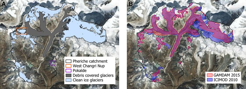
Figure 1. Study area: (a) location map of the Pheriche catchment (black) in the Sagarmatha National Park (green) in Nepal. Characteristics
of the meteorological stations are summarized in Table 1. (b) Hypsometric curve of the Pheriche catchment.
Figure 2. Daily minimal and maximal air temperatures and daily precipitation measured at the Pyramid station.
the outflow coming from glacierized areas. Here, flow com- moist summer with most of the annual precipitation occur-
ponents were estimated using two different definitions of the ring during the monsoon from June until September, and
hydrological contributions for assessing their relative contri- two transition seasons: the pre-monsoon season in April and
butions to the total water balance. Finally, model results are May and the post-monsoon season in October and November
analyzed at the annual, monthly, daily, and sub-daily scales (Shrestha et al., 2000). At 5000 m, the annual precipitation is
in order to explain the origin of the water flows and their sea- around 600 mm and the mean monthly temperature ranges
sonal and daily variations. from −8.4 ◦ C in January to 3.5 ◦ C in July, according to tem-
perature and precipitation data from the Pyramid EvK2 sta-
tion (Fig. 2 and Table 1). The hydrological regime follows
2 Study area the precipitation cycle with high flows during the monsoon
season, when most of the annual precipitation occurs, com-
This study focuses on the Pheriche sub-catchment of the
plemented by the melting of snow and ice, and low flows
Dudh Koshi basin (outlet at coordinates 27.89◦ N, 86.82◦ E)
during winter.
located in Nepal on the southern slopes of Mt. Everest in
Due to high elevation, vegetation in the catchment is
the Sagarmatha National Park (SNP) (Fig. 1). The catch-
scarce. The basin area is mainly covered by rocks and
ment area is 146 km2 and its elevation extends from 4260
moraines (43 %) (Bajracharya et al., 2010) and glaciers
to 8848 m a.s.l.
(43 %) (Racoviteanu et al., 2013). Only 14 % of the basin
Local climate is mainly controlled by the Indian sum-
area is covered by grasslands and shrublands. Glaciers be-
mer monsoon (Bookhagen and Burbank, 2006) and is char-
long to the summer-accumulation type (Wagnon et al., 2013)
acterized by four different seasons: a cold dry winter from
and are partially fed by avalanches (King et al., 2017;
December to March with limited precipitation, a warm and
www.hydrol-earth-syst-sci.net/23/3969/2019/ Hydrol. Earth Syst. Sci., 23, 3969–3996, 2019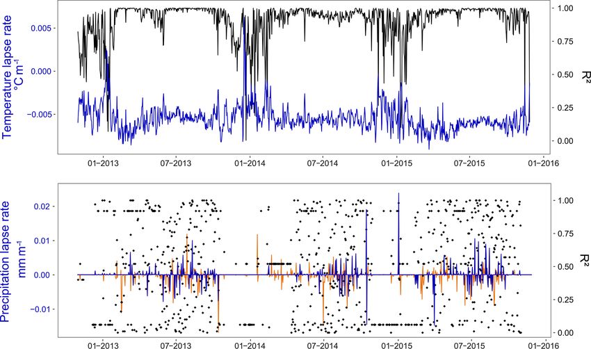
3972                           L. Mimeau et al.: Quantification of different flow components in the Dudh Koshi catchment

Figure 3. Glacier outlines in the Pheriche catchment. (a) Clean glaciers and debris-covered glaciers from Racoviteanu et al. (2013) and
location of the clean ice West Changri Nup and Pokalde glaciers, and (b) GAMDAM (red) and ICIMOD (blue) glacier outlines.

Table 1. Location of measurements. T : air temperature, P : precipitation, WS: wind speed, RH: relative humidity, SWin: incoming shortwave
radiation, SWout: outgoing shortwave radiation, LWin: incoming longwave radiation.

          No.   Name            Elevation (m)    Lat. (◦ )   Long. (◦ )   Measured parameters                  Manager
          1     Pangboche               3950     27.857        86.794     T, P                                 IRD
          2     Pheriche                4260     27.895        86.819     T , P , WS, RH, SWin                 EvK2-CNR, IRD
          3     Pyramid                 5035     27.959        86.813     T , P , WS, RH, SWin, SWout, LWin    EvK2-CNR, IRD
          4     Changri Nup             5363     27.983        86.779     SWin, SWout                          GLACIOCLIM

Sherpa et al., 2017); 60 % of the glaciers are located be-                boche station was recorded with a tipping bucket. Air tem-
tween 5000 and 6000 m a.s.l. Debris-covered glaciers are                  perature, wind speed, relative humidity, and shortwave and
found at low elevations mainly on the ablation tongues of the             longwave radiation at Pheriche and Pyramid were provided
glaciers (Fig. 3). According to the Racoviteanu et al. (2013)             by the EvK2-CNR stations.
glacier inventory, debris-covered glaciers represent 30 % of                 Discharge measurements of the Khumbu River at Pheriche
the glacierized area, with smaller melting rates at similar el-           have been obtained using a pressure water level sensor at a
evations to debris-free glaciers due to the insulating effect of          30 min time step since October 2010.
the debris layer (Vincent et al., 2016).                                     The MODImLab algorithm developed by Sirguey et al.
                                                                          (2009) was applied to MODIS reflectance data to obtain
                                                                          daily albedo and snow fraction satellite images for the pe-
3     Data and model setup                                                riod 2010–2015. We used the Sirguey et al. (2009) algo-
                                                                          rithm rather than the MOD10A1 500 m snow products be-
3.1    Database                                                           cause it generates daily regional snow cover images at 250 m
                                                                          resolution and applies corrections to atmospheric and topo-
To describe the topography of the study area, an ASTER                    graphic effects, which makes the snow cover maps more re-
DEM originally at 30 m resolution was resampled to a 100 m                alistic in mountainous areas. Twenty-seven cloud-free Land-
resolution. The SOTER Nepal soil classification (Dijkshoorn               sat8 images were used to generate snow maps at 30 m res-
and Huting, 2009) and a land-cover classification from ICI-               olution between 1 November 2014 and 31 December 2015.
MOD (Bajracharya, 2014) were used for the soil and land-                  A NDSI (Normalized-Difference Snow Index) threshold of
cover description.                                                        0.15 was taken to separate snow-free and snow-covered pix-
   Meteorological data were available at hourly time steps                els on Landsat8 data as proposed by Zhu and Woodcock
from three automatic weather stations (AWS) located                       (2012). Daily snow cover maps were then retrieved from the
at Pangboche (3950 m a.s.l.), Pheriche (4260 m a.s.l.), and               MODImLab snow fraction product: areas with a snow frac-
Pyramid (5035 m a.s.l.) (Table 1). Since December 2012, pre-              tion above 0.15 were defined as snow-covered areas so that
cipitation has been recorded at the Pheriche and Pyramid                  the MODImLab snow cover area (SCA) matches the Land-
AWS by two Geonor T-200 sensors designed to measure both                  sat8 SCA on the common dates. For the rest of this study
liquid and solid precipitation. Data were corrected for poten-            we call MODIS data albedo and snow cover data obtained
tial undercatch following the method used by Lejeune et al.               with the MODImLab algorithm. We also used snow albedo
(2007) and Sherpa et al. (2017). Precipitation at the Pang-

Hydrol. Earth Syst. Sci., 23, 3969–3996, 2019                                          www.hydrol-earth-syst-sci.net/23/3969/2019/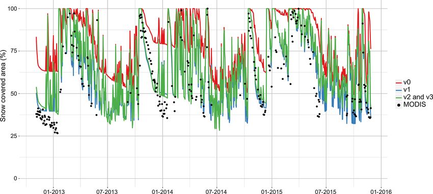
L. Mimeau et al.: Quantification of different flow components in the Dudh Koshi catchment                                                     3973

Table 2. Glacier outline characteristics.

                                                                   Satellite imagery         Acquisition      Spatial resolution of the satellite
  Glacier outline                           Area                   used for delineation      dates                 images used for delineation
  Racoviteanu et al. (2013)                 Dudh Koshi, Langtang   ASTER, IKONOS-2           2003–2008                                  1–90 m
  GAMDAM (Nuimura et al., 2015)             Asian glaciers         SRTM, LANDSAT             1999–2003                                30–120 m
  ICIMOD (Bajracharya et al., 2010)         Nepal                  IKONOS, LANDSAT,          1992–2006                                 1–120 m
                                                                   ASTER

data from in situ measurements at Pyramid and Changri Nup                 Frans et al., 2015). Distributed meteorological data (air tem-
(Table 1).                                                                perature, precipitation, relative humidity, wind speed, and
   To describe the glacierized area in the basin, we com-                 shortwave and longwave incoming radiation) are requested
pared three different glacier outlines available as vector lay-           as input, as well as distributed geographical information (el-
ers for the Khumbu region: the glacier delineation proposed               evation, soil type, land cover, soil depth, and ice thickness).
by Racoviteanu et al. (2013) specifically set up for the Dudh
Koshi basin; the GAMDAM inventory covering the entire                     3.2.2    Snow albedo parameterization
Himalayan range (Nuimura et al., 2015); and the ICIMOD
inventory (Bajracharya et al., 2010) (Fig. 3). The three out-             In the original DHSVM-GDM version, the snow albedo αs
lines have been derived on different grids, from different                (–) is set to its maximum value αsmax (to be fixed either by
datasets at different spatial resolutions and covering differ-            calibration or from observed albedo values) after a snowfall
ent temporal periods (see Table 2), thus leading to different             event and then decreases with time according to the follow-
results.                                                                  ing equations (Wigmosta et al., 1994):
                                                                                              0.58
   Mass balances estimated by Sherpa et al. (2017) for the                αs = αsmax (λa )N           if Ts < 0,
clean-ice West Changri Nup and Pokalde glaciers located
                                                                                             N 0.46
in the Pheriche basin (Fig. 3) were used as a reference, as               αs = αsmax (λm )            if Ts > 0,                                    (1)
well as mean annual glacier mass balances calculated over
                                                                          where N is the number of days since the last snowfall, λa (–)
the Pheriche basin area for the period 2000–2016 by Brun
                                                                          and λm (–) correspond to 0.92 and 0.70 for the accumulation
et al. (2017).
                                                                          season and the melt season, respectively, and Ts is the snow
                                                                          surface temperature (◦ C).
3.2     Glacio-hydrological modeling                                         MODIS albedo images and the albedo measurements from
                                                                          Pyramid and Changri Nup were used to analyze the decrease
3.2.1    General description of the model                                 in snow albedo with age in various locations of our study
                                                                          area. Figure 4 compares the observed albedo decay as a func-
The DHSVM-GDM (Distributed Hydrological Soil Vegeta-                      tion of time for snow events with at least 3 consecutive days
tion Model – Glaciers Dynamics Model) glacio-hydrological                 without clouds after the snowfall with the albedo parame-
model is a physically based, spatially distributed model                  terization in DHSVM-GDM. Since the observed values are
which was developed for mountain basins with rain and snow                not well represented by the standard albedo decrease, the
hydrological regimes (Wigmosta et al., 1994; Nijssen et al.,              parameterization was replaced by Eq. (2), with a decay of
1997; Beckers and Alila, 2004). A glacier dynamics module                 the albedo when there is no new snowfall inspired by the
was recently implemented in DHSVM by Naz et al. (2014)                    ISBA model albedo parameterization (Douville et al., 1995)
to simulate glacier mass balance and the runoff production                and with the fresh snow albedo modified as a function of the
in catchments with glaciers, thus extending the application to            amount of snowfall:
ice-dominated hydrological regimes. The resulting DHSVM-
GDM simulates the spatial distribution and the temporal evo-              αs = (αst−1 − αsmin ) exp(−cN ) + αsmin
lution of the principal water balance terms (soil moisture,                  if isnowfall = 0 mm h−1 ,
evapotranspiration, sublimation, glacier mass balance, snow
cover, and runoff) at hourly to daily timescales. It uses a two-          αs = max(0.6, αst−1 )
layer energy and mass balance module for simulating snow                     if 0 mm h−1 < isnowfall 6 1 mm h−1 ,
cover evolution and a single-layer energy and mass balance                                                                              isnowfall − 1
module for glaciers (Andreadis et al., 2009; Naz et al., 2014)            αs = max(0.6, αst−1 ) + (αsmax − max(0.6, αst−1 ))
                                                                                                                                            3−1
and has been applied in a number of studies for snow and
                                                                             if 1 mm h−1 < isnowfall 6 3 mm h−1 ,
cold region hydrology (e.g., Leung et al., 1996; Leung and
Wigmosta, 1999; Westrick et al., 2002; Whitaker et al., 2003;             αs = αsmax
Zhao et al., 2009; Bewley et al., 2010; Cristea et al., 2014;                if isnowfall > 3 mm h−1 ,

www.hydrol-earth-syst-sci.net/23/3969/2019/                                               Hydrol. Earth Syst. Sci., 23, 3969–3996, 2019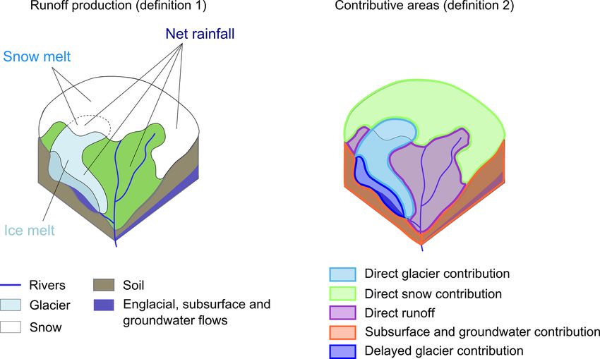
3974                          L. Mimeau et al.: Quantification of different flow components in the Dudh Koshi catchment

Figure 4. Original and modified parameterization of the snow albedo evolution in DHSVM-GDM and comparison with observed albedo data
(2010–2015) in Pheriche, Pyramid, and Changri Nup.

                                                             (2)            lope neighbor cells is larger than 50 cm: 95 % of the dif-
                                                                            ference is removed by avalanches.
where αst−1 is the albedo from the previous time step, αsmin
is the minimal snow albedo of 0.3 (estimated using the mean         The transfer of snow by avalanches is based on the surface
minimal albedo values observed at the station and on MODIS          runoff routing in DHSVM-GDM: at every time step start-
images), N is the number of days since the last snowfall, c is      ing from the highest cell of the DEM to the lowest, each cell
the coefficient of the exponential decrease (d−1 ), and isnowfall   can transfer snow to its closest downslope neighbor cells (be-
the snowfall intensity (mm h−1 ). Since the observed decrease       tween one and four cells). In case of several possible direc-
is dependent on elevation, the coefficient c is calculated as a     tions downstream, avalanche snow is distributed according
function of elevation according to Eq. (3):                         to a ratio based on the slope of each of the directions. Within
                                                                    the same time step, the amount of snow in the receiving cells
c = 20 exp(−0.001 Z),                                        (3)
                                                                    is actualized and the avalanches propagate downslope until
where Z is the elevation of the cell in m a.s.l.                    the conditions cited above are no longer respected.
   The new function for the decrease in the snow albedo is
also shown in Fig. 4.                                               3.2.4     Glacier parameterization

3.2.3   Avalanche parameterization                                  Distributed ice thickness is derived from the terrain slope fol-
                                                                    lowing the method described in Haeberli and Hölzle (1995).
Transport of snow by avalanches is not represented in                  In the original DHSVM-GDM version, glacier melt is in-
the original version of DHSVM-GDM. The absence of                   stantaneously transferred to the soil surface, which is pa-
avalanches in the model can lead to an unrealistic accumu-          rameterized as bedrock under glaciers (Naz et al., 2014).
lation of snow in steep high-elevation cells, where the air         This significantly underestimates the transfer time through
temperature remains below 0 ◦ C, and to a deficit of snow           glaciers. In this study, storage of liquid water inside glaciers
in the lower areas, where snowmelt occurs during the melt-          was implemented by adding an englacial porous layer be-
ing season. The simulated water balance directly depends on         tween the glacier and the bedrock allowing the liquid wa-
the snow cover; thus, not considering avalanches can lead to        ter storage within the glacier. Previous studies have shown
significant errors. In order to address these discrepancies, an     the good performance of adding a conceptual representation
avalanche module was implemented in DHSVM-GDM. The                  of the storage and drainage in the glaciers within glacio-
avalanche model transfers snow to downslope neighbor cells          hydrological models (e.g., Jansson et al., 2003; Hock and
under the following conditions:                                     Jansson, 2006). The most widely adopted approach is based
                                                                    on a reservoir or a cascade of reservoirs with time-invariant
  – if the terrain slope is steeper than 35◦ and the amount of
                                                                    parameters (e.g., Farinotti et al., 2012; Zhang et al., 2015;
    dry snow water equivalent (total snow water equivalent
                                                                    Hanzer et al., 2016; Gao et al., 2017). Here, storage of liq-
    minus liquid water content) is higher than 30 cm: 5 cm
                                                                    uid water inside glaciers was implemented by adding an
    of snow water equivalent remains in the cell and the rest
                                                                    englacial porous layer between the glacier and the bedrock
    is removed by avalanches;
                                                                    allowing the liquid water storage within the glacier. This
  – if the terrain slope is less steep than 35◦ but the differ-     englacial porous layer has a depth of 2 m and is characterized
    ence in snow water equivalent compared to the downs-            by a porosity of 0.8 and a hydraulic conductivity (vertical and

Hydrol. Earth Syst. Sci., 23, 3969–3996, 2019                                       www.hydrol-earth-syst-sci.net/23/3969/2019/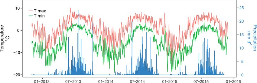
L. Mimeau et al.: Quantification of different flow components in the Dudh Koshi catchment                                      3975

lateral) of 3 × 10⁻⁴ m s−1 (see Table A2). As in the previ-            In order to evaluate the seasonal components of the out-
ously cited studies, the parameters are kept constant through       flow at the catchment’s outlet, we also define the hydrologi-
the simulations. They were optimized here according to the          cal contributions as fractions of the outflow coming from the
constraint of minimizing the differences (in terms of least         different contributing areas (definition 2):
squares) between the recession shape of the simulated hy-
                                                                      – direct glacier contribution: direct runoff from glacier-
drographs and the observed one.
                                                                        ized areas;
   Moreover, since the standard DHSVM-GDM model does
not take into account the impact of the debris layer on melt-         – delayed glacier contribution: resurging meltwater stored
ing of the glaciers, the insulating effect of the debris layer is       inside glaciers;
not represented. Here, we implemented a reduction factor for
ice melt generated in grid cells with debris-covered glaciers         – direct snow contribution: direct outflow from snow-
(see Sect. 3.3).                                                        covered non-glacierized areas;
                                                                      – direct runoff: direct runoff from areas without snow and
3.2.5   Quantification of the flow components
                                                                        glaciers; and
Quantifying the relative contributions of ice melt, snowmelt,         – subsurface and groundwater contribution: resurging wa-
and rainfall in the river discharge at different timescales is          ter from the soil in non-glacierized areas resulting from
a difficult task because hydrological models usually do not             infiltrated rainfall, snowmelt, as well as upstream lateral
track the origin of water during transfer within the catch-             subsurface flows.
ment (Weiler et al., 2018). There are also different ways of
defining the origins of the streamflow. Weiler et al. (2018)        These contributions are obtained from the amount of water
lists three types of contributions: (1) contributions from the      reaching the soil surface simulated by DHSVM-GDM (see
source areas, i.e. from each class of land cover, (2) contribu-     Supplement). On each grid cell, this volume is a mixture of
tions from the runoff generation (overland flow, subsurface         ice melt, snowmelt, and rainfall and can either infiltrate into
flow, and groundwater flow), and (3) input contributions (ice       the soil or produce runoff. Definition 2 combines contribu-
melt, snowmelt, and rain).                                          tions from source areas (glacierized and non-glacierized ar-
   In this study, two different definitions were used to esti-      eas) and contributions from runoff generation (direct runoff,
mate the hydrological contributions. First, we estimate the         englacial contribution, and soil contribution).
contributions of ice melt, snowmelt, and net rainfall to the           Figure 5 illustrates the two definitions of the different con-
total water input (definition 1) according to the following         tributions to outflows. Definition 1 allows assessment of the
water balance equations (all the terms are fluxes expressed         annual impact of glacier melt and snowmelt on the water pro-
in L T−1 ):                                                         duction, while definition 2 describes the intra-annual rout-
                                                                    ing of the water within the catchment. Moreover, using the
Input = Icemelt + Snowmelt + RainNet,                        (4)    two definitions allows us to directly compare the results with
dIwq                                                                other hydrological modeling studies in the Dudh Koshi basin,
        = GlAcc − Icemelt − SublIce,                         (5)    which have estimated glacier contributions either from ef-
  dt
                                                                    fective ice melt (Savéan et al., 2015; Ragettli et al., 2015;
dSwq
        = Psolid − Snowmelt − SublIce − GlAcc,               (6)    Soncini et al., 2016) or runoff from glacierized areas (Im-
  dt                                                                merzeel et al., 2012; Nepal et al., 2014). Further, we assessed
RainNet = Pliquid − Eint ,                                   (7)    the impact of the definition of hydrological components on
dStorage                                                            the estimated glacier contribution.
           = Input − Q − ET ,                                (8)
     dt                                                                Flow components were estimated for the period 2012–
                                                                    2015 at annual scale, on the basis of the glaciological year
        dI        dS
where dtwq and dtwq are the variations of the ice and snow          (from 1 December to 30 November), as well as monthly,
storages, GlAcc is the amount of snow that is transferred to        daily, and sub-daily scales, in order to have a better under-
the ice layer by compaction on glaciers (Naz et al., 2014),         standing of the seasonal variation of the estimated hydrolog-
SublIce and SublSnow are the amounts of sublimation from            ical contributions.
the ice and snow layers, Psolid and Pliquid are the amounts
of solid and liquid precipitation, and Eint is the amount of        3.3   Experimental setup
evaporation from intercepted water stored in the canopy. It is
worth noting that the sum of these contributions (Input) is not     Simulations were run with a 1 h time step and a spatial res-
equal to the outflow at the catchment outlet Q as it represents     olution of 100 m for the period from 1 November 2012 to
all liquid water reaching the soil surface (before                  27 November 2015 corresponding to the period with the most
                                                infiltration
                                                                   available meteorological and discharge data.
and potential storage in the soils and glaciers dStorage
                                                     dt    and
                                                                       A soil depth map was derived from the DEM using
before evapotranspiration (ET )).                                   the method proposed in the DHSVM-GDM documentation

www.hydrol-earth-syst-sci.net/23/3969/2019/                                      Hydrol. Earth Syst. Sci., 23, 3969–3996, 2019
3976                           L. Mimeau et al.: Quantification of different flow components in the Dudh Koshi catchment

Figure 5. Definitions of the flow components.

(Wigmosta et al., 1994). As a result, soil depth outside            porous layer parameters (depth, porosity, and hydraulic con-
glacierized areas ranges between 0.5 and 1 m (glaciers are          ductivity) and avalanche parameters was also performed (see
considered to lay on bedrock). All parameter values retained        Table B1 for the tested parameter values) and the relative im-
for the simulations (with no calibration) are summarized in         pact on the simulated hydrological response was discussed
Appendix A.                                                         (see Sect. 5.3.2).
   In order to test the impact of the representation of the            The sensitivity to the values of the englacial porous layer
cryospheric processes on the hydrological modeling, we per-         parameters (depth, porosity, and hydraulic conductivity), as
formed simulations with the four following configurations:          well as to the values of the avalanche parameters and to the
                                                                    soil depth is also analyzed in the discussion section of the
  – v0: original DHSVM-GDM snow and glacier parame-                 paper.
    terization;
                                                                    3.3.1   Model forcing
  – v1: modified snow albedo parameterization;
  – v2: modified snow albedo parameterization and                   Meteorological data from the Pheriche and Pyramid stations
    avalanche module;                                               (Table 1) were spatialized over the basin by an inverse dis-
                                                                    tance interpolation method. Altitudinal lapse rates of precip-
  – v3: modified snow albedo parameterization, avalanche            itation and temperature were calculated at a 1 h time step
    module, and melt coefficient for debris-covered                 from data collected at Pangboche (3950 m a.s.l.), Pheriche
    glaciers.                                                       (4260 m a.s.l.), and Pyramid (5035 m a.s.l.) (Fig. 6). Only
                                                                    significant lapse rates with R 2 values higher than 0.75 were
All four configurations were run with the Racoviteanu et al.
                                                                    retained for precipitation (43 % of the dataset). For smaller
(2013) glacier outline. Concerning the melt of the debris-
                                                                    R 2 , the lapse rate is considered not significant and thus set to
covered glaciers, we use a reduction factor of 0.4 as esti-
                                                                    0.
mated by Vincent et al. (2016) from a study on uncovered
                                                                       In this study, the precipitation lapse rates show a large sea-
and debris-covered areas of the Changri Nup glacier.
                                                                    sonal variability with daily lapse rates ranging from −41
   Using configuration v3, we also tested the impact of us-
                                                                    to 9 mm km−1 . Precipitation decreases with elevation dur-
ing different glacier outlines (the GAMDAM and ICIMOD
                                                                    ing the monsoon season and increases with elevation in win-
inventories were also considered for simulations) and ana-
                                                                    ter: during the simulation period, we found 450 days (40 %)
lyzed the sensitivity related to different values of parameters
                                                                    with no precipitation, 83 days (8 %) with a strictly negative
related to the cryospheric processes (see Table B1). Indeed,
                                                                    lapse rate, and 165 days (15 %) with a strictly positive lapse
the debris-covered glacier melt reduction factors estimated
                                                                    rate. Concerning temperatures, daily lapse rates range from
in Konz et al. (2007), Nepal et al. (2014), and Shea et al.
                                                                    −0.009 to +0.006 ◦ C m−1 . We found only 10 days (1 %)
(2015) are, respectively, equal to 0.3, 0.33, and 0.47. Thus,
                                                                    showing a temperature inversion with a positive daily lapse
values between 0.3 and 0.5 were also considered (in addition
                                                                    rate.
to the reference of 0.4). A sensitivity analysis of the englacial

Hydrol. Earth Syst. Sci., 23, 3969–3996, 2019                                     www.hydrol-earth-syst-sci.net/23/3969/2019/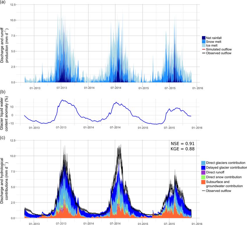
L. Mimeau et al.: Quantification of different flow components in the Dudh Koshi catchment                                               3977

Figure 6. Daily temperature and precipitation lapse rates. Discarded precipitation lapse rates (with a R 2 < 0.75) are represented in orange.

3.3.2    Model evaluation                                                on the simulated annual outflow, the daily SCA, and annual
                                                                         glacier mass balances.
A multi-criteria evaluation was made considering simulated
outflows, SCA, and glacier mass balances. Discharge mea-                 4.1.1    Annual outflow
surements at Pheriche station were used as a reference for the
evaluation of simulated outflows. A 15 % confidence inter-
                                                                         Figure 7 represents the annual outflow and flow components
val was retrieved as representative of the uncertainty of mea-
                                                                         (definition 1) simulated with the different model configura-
sured discharge. Nash–Sutcliffe efficiency (NSE) (Nash and
                                                                         tions, indicating the impact of each modification of the snow
Sutcliffe, 1970) and Kling–Gupta efficiency (KGE) (Gupta
                                                                         and glacier parameterization on the simulated annual out-
et al., 2009) were chosen as objective functions and applied
                                                                         flow and flow components. Configuration v1 leads to a drasti-
to daily discharges. The simulated SCA was evaluated in
                                                                         cally increased outflow due to an enhanced ice melt compo-
comparison to daily SCA derived from MODIS images. Be-
                                                                         nent. Implementing the avalanche module (v2) reduces the
cause a large number of MODIS images suffer from cloud
                                                                         ice melt component and increases the snowmelt component
coverage, we only compared the simulated and observed
                                                                         by 21 %. Configuration v3 including debris-covered glaciers
SCA during days with less than 5 % of cloud cover in the
                                                                         further reduces the ice melt, resulting in a simulated annual
catchment. The simulated glacier mass balances were evalu-
                                                                         outflow close to the observations.
ated at basin scale by a comparison with published regional
                                                                            Figure 7 shows that configuration v2, which does not con-
geodetic mass balances and at local scale using available
                                                                         sider the debris-covered glaciers, overestimates the outflow
stake measurements on the clean ice West Changri Nup and
                                                                         at Pheriche with a mean bias of +32 % compared to the
Pokalde glaciers (Sherpa et al., 2017).
                                                                         annual observed outflow. Without the debris layer, the ice
                                                                         melt component represents 817 mm, which is nearly twice
                                                                         the amount of ice melt obtained with v3 that includes debris-
4     Results                                                            covered glacier melt.
                                                                            The configuration with all three modifications (v3) gives
4.1     Impact of the snow and glacier parameterizations                 results similar to the original parameterization of DHSVM-
        on the simulated results                                         GDM (v0) in terms of glacier mass balance, improving
                                                                         slightly the annual outflow. The ice melt factor for debris-
This section presents the simulation results obtained with the           covered glaciers and the avalanches compensate for the in-
different configurations of the DHSVM-GDM model (con-                    crease in ice melt caused by the new snow albedo parame-
figurations v0, v1, v2, and v3; see Sect. 3.2.5) and the anal-           terization, but the modifications implemented in v3 impact
ysis of the impact of the snow and glacier parameterizations             the results for the flow components: on average, less ice melt

www.hydrol-earth-syst-sci.net/23/3969/2019/                                             Hydrol. Earth Syst. Sci., 23, 3969–3996, 2019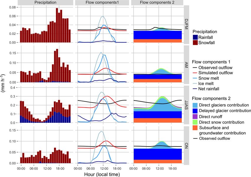
3978 L. Mimeau et al.: Quantification of different flow components in the Dudh Koshi catchment
Figure 7. Simulated annual hydrological contributions (definition 1) to Pheriche outflow for 3 glaciological years from December 2013 to
November 2015.
Table 3. NSE and KGE values calculated on the daily discharges on ward and corrects the lack of snow observed with configu-
the period 2012–2015 for each model configuration. ration v1 at the edges of the permanent snow cover (Fig. 9).
The results for the SCA and snow cover duration using con-
v0 v1 v2 v3 figuration v3 show no difference compared to configuration
NSE 0.87 0.53 0.74 0.91 v2 since only the ice melt rate for debris-covered glaciers is
KGE 0.83 0.5 0.65 0.88 modified.
4.1.3 Glacier mass balances
and more snowmelt are generated. Moreover, configuration Figure 10 compares the simulated mean annual glacier
v3 modifies the seasonal variation of the outflow by increas- mass balances obtained with the different model configura-
ing winter discharges and reducing monsoon discharges (not tions with mass balances determined with geodetic meth-
illustrated here), which improves the daily NSE and KGE ods between 1999 and 2015 (Bolch et al., 2012; Gardelle
(Table 3). et al., 2013; Nuimura et al., 2015; King et al., 2017; Brun
et al., 2017). These geodetic mass balances range from
4.1.2 Snow cover dynamics −0.67±0.45 m w.e. yr−1 (2000–2008) (Nuimura et al., 2015)
to −0.32±0.09 m w.e. yr−1 (2000–2015) (Brun et al., 2017).
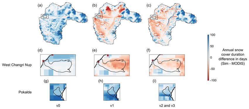
Figures 8 and 9 compare the simulated SCA and duration ob- Our results show that the snow parameterization has
tained with configurations v0, v1, v2, and v3 to data derived a significant impact on the simulated glacier mass bal-
from MODIS images. The SCA is strongly overestimated us- ance. The mass balance simulated with v0 is on average
ing the original parameterization v0: Fig. 8 shows that after −0.82 m w.e. yr−1 and decreases to −2.02 m w.e. yr−1 with
full coverage it does not decrease fast enough compared to the corrected snow albedo (v1) since the modified snow
MODIS data. Figure 9 demonstrates that the snow cover du- albedo parameterization accelerates the snowmelt, which
ration is overestimated for the entire catchment area. This in- leads to more uncovered ice and stronger glacier melt. The
dicates that in the simulations snow does not melt fast enough avalanche module (v2) adds snow on glaciers and increases
with the original parameterization. Configuration v1 with the the accumulation and, thus, reduces the glacier melt to
modified snow albedo parameterization (Eq. 2) accelerates −1.69 m w.e. yr−1 . Nevertheless, the mass balance remains
the snowmelt and improves the SCA simulation (Fig. 8). The too negative compared to geodetic mass balances, which sug-
RMSE between the simulated and observed SCA decreases gests that the model produces too much ice melt. The imple-
from 29 % using v0 to 14 % using v1 and v2. Figure 9 shows mentation of debris-covered glaciers (v3) gives a mean an-
that with configuration v1 in some areas located at high ele- nual glacier mass balance of −0.84±0.14 m w.e. yr−1 , which
vation the snow cover duration is underestimated. This bias is within the intervals of uncertainty and thus in good agree-
is rectified in configuration v2 since the avalanche module ment with geodetic methods.
transfers snow from high-elevation and sloping cells down-
Hydrol. Earth Syst. Sci., 23, 3969–3996, 2019 www.hydrol-earth-syst-sci.net/23/3969/2019/L. Mimeau et al.: Quantification of different flow components in the Dudh Koshi catchment 3979 Figure 8. Comparison of the MODIS SCA and the simulated daily SCA with the four modeling configurations (v0, v1, v2, and v3) for the Pheriche catchment. Figure 9. Difference between the mean annual snow cover duration simulated with DHSVM-GDM and derived from MODIS images (in days) for the Pheriche catchment (a–c), with a focus on West Changri Nup (d–f) and Pokalde glaciers (g–i). We also evaluated the mass balance at the point scale. Fig- figuration v0, the model overestimates the point mass bal- ure 11 shows the simulated mass balances with parameteriza- ances because of small snowmelt rates (see also Sect. 4.1.2). tions v0, v1, v2, and v3 versus the observed mass balances of With configuration v1, the model overestimates the ice melt the two debris-free glaciers West Changri Nup and Pokalde on the West Changri Nup glacier due to a lack of accumula- measured in situ for the 3 glaciological years (2012–2015). tion in the western part of the catchment and a too strong ac- Here, configuration v3 gives the same results as configura- cumulation on the Pokalde glacier (Fig. 9). Configuration v2 tion v2 because in configuration v3 only the ice melt rate on improves the simulated mass balance by transferring snow debris-covered glaciers is modified. The simulated mass bal- due to avalanches on the West Changri Nup glacier and by re- ances vary according to the model configuration. With con- moving excessive snow accumulation on the Pokalde glacier. www.hydrol-earth-syst-sci.net/23/3969/2019/ Hydrol. Earth Syst. Sci., 23, 3969–3996, 2019
3980                           L. Mimeau et al.: Quantification of different flow components in the Dudh Koshi catchment

Figure 10. Mean annual glacier mass balances simulated with configurations v0, v1, v2, and v3. The error bar for configuration v3 represents
the uncertainty related to the debris layer coefficient melt varying between 0.3 and 0.5.

Figure 11. Annual simulated and measured point mass balances on West Changri Nup (a) and Pokalde (b) glaciers; also shown is the 1 : 1
line.

For the Pokalde glacier, the mass balances simulated with               ertheless, regarding point mass balances, the agreement is far
configuration v3 show a larger variability than the mass bal-           from being perfect, due either to simulation errors (including
ances simulated with configuration v0, but the point mass               errors depending on the interpolated input fields and errors
balances are spread around the diagonal axis, which leads to            induced by the representation of slopes and expositions by
a bias 10 times smaller (mean bias of 1 m with v0 and 0.1 m             the DEM) or a lack of representativeness of the measure-
with v3).                                                               ments.
   The results at basin scale and point scale show that the
snow parameterization has a strong impact on the simulated              4.2    Simulated outflow and flow components
glacier mass balance and that the new snow albedo param-
eterization and the avalanching module clearly improve the
                                                                        This section presents the outflows and flow components sim-
simulated glacier mass balance on debris-free glaciers. Nev-
                                                                        ulated in the Pheriche basin during the period 2012–2015

Hydrol. Earth Syst. Sci., 23, 3969–3996, 2019                                          www.hydrol-earth-syst-sci.net/23/3969/2019/
L. Mimeau et al.: Quantification of different flow components in the Dudh Koshi catchment 3981
Figure 12. Simulated annual hydrological contributions to Pheriche outflow for the two definitions of the flow components (definition 1 and
definition 2) and for 3 glaciological years from December 2013 to November 2015.
Table 4. Annual hydrological balance simulated with configuration v3 for 3 glaciological years from December 2013 to November 2015.
2013 2014 2015
Total precipitation (mm) 708 644 683
Snowfall (mm) 501 492 561
Observed discharge Qobs (mm) 994 1081 786
Qobs ±15% (mm) 845–1143 919–1244 668–904
Simulated discharge Qsim (mm) 999 933 729
Bias (%) +1 −14 −7
Evapotranspiration (mm) 61 48 43
Sublimation (mm) 91 96 97
Flow components (definition 1)
Net rainfall (mm) 164 117 93
Snowmelt (mm) 420 368 362
Ice melt (mm) 476 496 317
Flow components (definition 2)
Direct glacier contribution (mm) 293 244 164
Delayed glacier contribution (mm) 414 420 304
Direct runoff (mm) 21 14 9
Direct snow contribution (mm) 51 55 43
Subsurface and groundwater contribution (mm) 220 200 211
with the modified version of DHSVM-GDM (configura- the annual observed outflows since they remain within the
tion v3). The simulation results are analyzed using two dif- 15 % interval of estimated error (Fig. 12 and Table 4).
ferent definitions of the flow components (definitions 1 and The results show an inter-annual variability of the flow
2; see Sect.3.2.5). components. During the period 2013–2015, the ice melt com-
ponent ranged from 41 % to 50 %, the snowmelt component
from 37 % to 47 %, and the net rainfall component from
4.2.1 Annual simulated outflow and hydrological
12 % to 16 %. These variations are related to the meteoro-
contributions
logical annual variability. The amount of rainfall decreased
from 2013 to 2015 and explains the decrease in the net rain-
The annual outflows simulated with the new parametrization fall components from 155 mm in 2013 to 88 mm in 2015.
of the model (configuration v3) are in good agreement with
www.hydrol-earth-syst-sci.net/23/3969/2019/ Hydrol. Earth Syst. Sci., 23, 3969–3996, 20193982 L. Mimeau et al.: Quantification of different flow components in the Dudh Koshi catchment
The snowmelt component is higher in 2013 because of the July and August during the monsoon season. During these 2
warmer pre-monsoon and monsoon seasons. The ice melt months, 24 % of the runoff is generated by net rainfall, 37 %
component is mainly controlled by the amount of winter by snowmelt, and 38 % by ice melt. From October to January,
snowfall. In 2014 a low amount of snowfall was observed, the runoff is produced by ice melt (up to 80 % in December)
so the snowpack melted more rapidly and the glaciers started and snowmelt (between 20 % and 30 %). Groundwater and
melting earlier. In contrast, 2015 was a year with a lot of win- englacial water represent a significant fraction of the monthly
ter snowfall, which delayed the beginning of the glacier melt outflow as they contribute more than 50 % of the outflow dur-
and explains the lower ice melt component. The losses by ing the monsoon season and can contribute up to 90 % dur-
evaporation and sublimation are rather constant through the ing winter (Fig. 14b). Direct contributions from glacierized
simulation period, ranging from 140 to 150 mm yr−1 . areas, snow areas, and direct runoff are highest during the
The runoff coefficients (ratio between the annual outflow monsoon season, when the englacial and soil storage is satu-
and annual precipitation) were on average equal to 1.4, which rated.
means that a considerable amount of water is withdrawn each
year from the catchment through ice melt (eventually in the 4.2.3 Diurnal cycle
form of a delayed groundwater flow).
On average, we find that the outflow is mainly produced by Figure 15 presents the diurnal cycles of precipitation and
meltwater as 46 % of the annual water input is due to ice melt hydrological components averaged for each considered sea-
and 41 % to snowmelt (definition 1). The contributions esti- son (winter, pre-monsoon, monsoon, and post-monsoon) ob-
mated according to definition 2 show the importance of infil- tained with configuration v3. During winter, pre-monsoon,
tration and subsurface flows in the water balance since more and post-monsoon, the observed outflow is rather constant
than 40 % of the outflow was coming from water infiltrated during the day, with a weak peak around noon when the tem-
in glaciers and more than 20 % from subsurface and ground- perature is at its maximum. During this period, almost all
water flows generated outside the glacier-covered area. of the precipitation is in the form of snowfall leading to no
The choice of the definition of the hydrological compo- direct response for the outflow. The peak around noon can
nents leads to different perceptions of the glacier contribution be explained by snowmelt or the melting of small frozen
to the outflow. The glacier contribution to the total outflow is streams. During the monsoon season, there is a strong di-
69 % if the contribution from the entire glacierized area (i.e. urnal cycle of the precipitation, with a maximum occurring
contributions of ice melt, snowmelt, and net rainfall) is con- during late afternoon or at night causing a peak in the dis-
sidered like in definition 2. However, the contribution from charge around midnight.
ice melt alone, included in definition 1, corresponds to only The model simulates ice and snowmelt during day time
46 % of the water input. with a maximum at noon as expected. Except for the mon-
soon season, it seems to simulate accurately the baseflow
4.2.2 Seasonal variations of the flow components during night without melt production: the discharge is rather
controlled by the release of the glacier and soil storage. How-
Figure 13 presents the daily simulated discharges simulated ever, the model simulates a peak of discharge around 14 h
with configuration v3 and the flow components estimated originating mostly from glacierized areas, 2 h after the maxi-
with the two different definitions. Daily discharges were well mum of ice and snowmelt, which does not correspond to ob-
simulated for 2012–2013 and 2014–2015 by the model, with served discharges. At daily and longer timescales the water
NSE equal to 0.91 and KGE equal to 0.88. However, the out- balance is correctly simulated. However, at a sub-daily scale
flow is underestimated by the model during the monsoon sea- the model responds too quickly to the snowmelt and ice melt
son in 2014. production.
The simulated total water input (i.e. the sum of snowmelt,
ice melt, and net rainfall) is always higher than the simulated 5 Discussion
outflow at the catchment outlet before the monsoon season
(from February to June) and lower during the post-monsoon 5.1 Simulation of the discharges and flow components
and winter seasons. This is mainly due to glacier meltwater
stored inside the glaciers during the pre-monsoon and mon- Soncini et al. (2016) studied flow components in the Pheriche
soon seasons and continuing surging during winter, as well catchment for the period 2013–2014 and estimated an an-
as to changes in the soil water storage (Figs. 13b and 14b). nual ice melt component of 55 % and a snowmelt component
Figure 14 shows the mean monthly flow components av- of 20 % of the annual outflow. The ice melt components are
eraged over the simulation period. From February to May– thus quite similar in terms of relative contributions to out-
June, the water input is entirely controlled by snowmelt and flow, which is not the case for the snowmelt components. We
ice melt (snowmelt between 50 % and 60 %, ice melt be- think that the main reason for such a difference is that we
tween 40 % and 48 %; Fig. 14a). The net rainfall, snowmelt, use different precipitation input. Indeed, precipitation data
and ice melt absolute contributions are at their maxima in are measured here by Geonor sensors, while in Soncini et al.
Hydrol. Earth Syst. Sci., 23, 3969–3996, 2019 www.hydrol-earth-syst-sci.net/23/3969/2019/L. Mimeau et al.: Quantification of different flow components in the Dudh Koshi catchment 3983 Figure 13. Daily discharges and flow components simulated with configuration v3: (a) production of ice melt, snowmelt, and net rainfall (note that the sum of the flow components represents the total water input and is not equal to the discharge at the catchment outlet; see definition 1, Sect. 3.2.5), (b) relative difference between the simulated glacier liquid water content and the inter-annual mean, and (c) hydrological contributions to the outflow (definition 2, Sect. 3.2.5). Observed discharges are represented by the black line with a 15 % interval of error. (2016) precipitation data come from tipping buckets. At the and mixed contributions of snowmelt and ice melt during Pyramid station, where both sensors are installed, the Geonor the post-monsoon and winter seasons. The studies of Raget- sensor measures 60 % more precipitation than the tipping tli et al. (2015) and Racoviteanu et al. (2013) concerning bucket over the period 2013–2015, and the main differences the Upper Langtang and the Dudh Koshi basin, respectively, are in terms of solid precipitation (Mimeau et al., 2019). showed that most of the winter outflow surges from soil, Concerning the seasonal contributions to the outflow, our channel, surface, and englacial storage changes, which is results are consistent with the results from Soncini et al. consistent with our results. However, the estimated flow com- (2016), who found a main contribution of snowmelt dur- ponents presented in this study, particularly the soil and ing the pre-monsoon season, mixed contributions of rain- englacial contributions, strongly depend on the model setup. fall, snowmelt, and ice melt during the monsoon season, Figure 13 shows that the main part of the soil infiltrated water www.hydrol-earth-syst-sci.net/23/3969/2019/ Hydrol. Earth Syst. Sci., 23, 3969–3996, 2019
3984                           L. Mimeau et al.: Quantification of different flow components in the Dudh Koshi catchment

Figure 14. Average monthly contributions to the water input (definition 1, Sect. 3.2.5) (a) and hydrological contributions (definition 2,
Sect. 3.2.5) (b) simulated with configuration v3 for the years 2012–2015.

Figure 15. Mean hourly precipitation, discharge, and flow components simulated with configuration v3 and averaged for the winter (DJFM),
pre-monsoon (AM), monsoon (JJAS), and post-monsoon (ON) seasons. Note the different y axis scales for each season.

Hydrol. Earth Syst. Sci., 23, 3969–3996, 2019                                        www.hydrol-earth-syst-sci.net/23/3969/2019/
L. Mimeau et al.: Quantification of different flow components in the Dudh Koshi catchment                                   3985

resurges within a day, whereas liquid water can be stored for         The results also showed that the modification of one spe-
several months within the glaciers. This difference between        cific hydrological process (here, the representation of the
the response of the soil storage and the englacial storage re-     snow albedo evolution) can have a significant impact on
sults from the soil and glacier parameterization (see the sen-     the simulated hydrological response of the catchment and
sitivity analysis in Sect. 5.3.2).                                 requires improvement of other processes (here, consider-
   At hourly scale, the results show that the model cannot         ing specific representation of avalanches and debris-covered
represent the diurnal cycle of the outflow correctly as the        glaciers).
simulated hydrological response is anticipated. Irvine-Fynn           Further modifications of the model could also lead to dif-
et al. (2017) found that on the Khumbu glacier the pres-           ferent model results, and it is also not excluded that differ-
ence of supraglacial ponds buffers the runoff by storing di-       ent model errors are compensating for each other. For exam-
urnally more than 20 % of the discharge. This could explain        ple, the results showed that the original model version leads
the longer transfer time observed on the measured outflows         to a correct simulation of the river discharges because the
which are not represented by the model. This shows that            non-representation of the insulation effect for debris-covered
the current representation of the glacier storage in DHSVM-        glaciers on the ice melt was compensated for by the incor-
GDM does not allow us to reproduce accurately the diurnal          rect representation of the snow albedo decrease. Due to the
variations of discharge, and further studies are needed in or-     complexity of the model and the represented processes, no
der to improve the model.                                          guarantee can be given that similar compensating effects still
   Overall, the comparison between the two definitions of the      occur in the model. In this study, the validation of the model
hydrological contributions shows that contributions must be        output was extended beyond the annual river discharge to dis-
explicitly specified in order to allow inter-comparison be-        charges at different timescales, the snow-covered area, and
tween models, especially for catchments with a large glacier-      glacier mass balances in order to validate the simulations of
ized area. Moreover, the use of two different definitions al-      the snow cover, glacier melt, and discharges separately. The
lows us to get complementary information on the origin of          results demonstrate that the new version of the model per-
the outflow (processes at the origin of the runoff, types of       forms well for all three signals. Moreover, the new parame-
flow generation, contributive zones). A perspective to im-         terizations of the snow albedo and ice melt under debris were
prove the quantification of the hydrological contributions to      based on observed data (MODIS and in situ albedo measure-
the outflow is to track the ice melt, snowmelt, and rainfall       ments, and coefficient for ice melt under debris from Vincent
component pathways in the model as suggested in Weiler             et al., 2016) and do not result from a calibration in order to
et al. (2018). This would enable us to quantify the fractions of   avoid compensation effects. Therefore, it is very likely that
the three components contributing to subsurface and ground-        the new implementation improved the quality of the repre-
water flow, which is not possible with the current version of      sented processes.
DHSVM-GDM.                                                            The results presented in this study also indicate potential
                                                                   future improvements to increase the reliability and to reduce
5.2   Representation of the cryospheric processes in the           the uncertainty of the simulations at short time steps. While
      model                                                        at daily and longer timescales the different hydrological com-
                                                                   ponents seem to be well reproduced by the model, the analy-
One of the main difficulties in glacio-hydrological model-         sis of the diurnal cycle (Fig. 15) shows that DHSVM-GDM
ing is to correctly simulate both river discharges, snow cover     responds too rapidly to the ice melt production, with too high
dynamics, and glacier mass balances. The results showed            diurnal peak discharges. This is probably related to the use of
that two different representations of the cryospheric pro-         constant parameters in the parameterization of the englacial
cesses in the model (v0 and v3) can lead to similar simu-          porous layer for glacier storage. Taking into account the sea-
lated annual outflows but different estimations of the ice melt    sonal variation of the efficiency of the englacial drainage
and snowmelt contributions. This is particularly true for the      system appears necessary to simulate the diurnal flow cycle
glaciological year 2014–2015, when the ice melt contribu-          correctly (Hannah and Gurnell, 2001). Therefore, further im-
tion decreases from 59 % with v0 to 41 % with v3 and the           provements should be based on studies analyzing the mecha-
snowmelt contribution increases from 29 % to 47 % (Fig. 7).        nisms of glacier drainage systems in the Khumbu region and
This can be explained by the fact that 2014–2015 was a year        their influence on glacier outflows (e.g., Gulley et al., 2009;
with a high amount of snowfall (Fujita et al., 2017); there-       Benn et al., 2017). These studies show that englacial con-
fore, the representation of snow processes in the model has a      duits and supraglacial channels, ponds, and lakes play a key
larger impact on the simulated runoff production than the 2        role in the response of glaciers: DHSVM-GDM could thus be
other years. This highlights the importance of a correct repre-    upgraded by implementing a parameterization of such sys-
sentation of snow processes in the model. This also shows the      tems and delay the response of glacierized areas, as success-
need to use as much validation data as possible to assess the      fully proposed, for instance, in the model developed by Flow-
coherence between the ice, snow, and hydrological processes        ers and Clarke (2002). Other processes such as supraglacial
and reduce the uncertainty in the flow component estimation.       ponds and ice cliffs melting, transport of snow by wind, or

www.hydrol-earth-syst-sci.net/23/3969/2019/                                     Hydrol. Earth Syst. Sci., 23, 3969–3996, 2019
You can also read