Impact of precipitation and increasing temperatures on drought trends in eastern Africa
←
→
Page content transcription
If your browser does not render page correctly, please read the page content below
Earth Syst. Dynam., 12, 17–35, 2021
https://doi.org/10.5194/esd-12-17-2021
© Author(s) 2021. This work is distributed under
the Creative Commons Attribution 4.0 License.

        Impact of precipitation and increasing temperatures on
                   drought trends in eastern Africa
              Sarah F. Kew1,6 , Sjoukje Y. Philip1,6 , Mathias Hauser2 , Mike Hobbins3,4 , Niko Wanders5 ,
       Geert Jan van Oldenborgh6 , Karin van der Wiel6 , Ted I. E. Veldkamp1 , Joyce Kimutai7 , Chris Funk8,9 ,
                                              and Friederike E. L. Otto10
                   1 Institute for Environmental Studies, Vrije Universiteit, Amsterdam, the Netherlands
                     2 Institutefor Atmospheric and Climate Science, ETH Zurich, Zurich, Switzerland
                   3 Cooperative Institute for Research in Environmental Sciences, University of Colorado

                                               Boulder, Boulder, Colorado, USA
           4 Physical Sciences Laboratory, NOAA/Earth System Research Laboratories, Boulder, Colorado, USA
                      5 Department of Physical Geography, Utrecht University, Utrecht, the Netherlands
                        6 Royal Netherlands Meteorological Institute (KNMI), De Bilt, the Netherlands
                                     7 Kenya Meteorological Department, Nairobi, Kenya
      8 U.S. Geological Survey Center for Earth Resources Observation and Science, Sioux Falls, South Dakota, USA
            9 Department of Geography, University of California, Santa Barbara, Santa Barbara, California, USA
                       10 School of Geography and the Environment, University of Oxford, Oxford, UK

                                   Correspondence: Sarah F. Kew (sarah.kew@knmi.nl)

                                   Received: 29 April 2019 – Discussion started: 24 May 2019
                      Revised: 8 September 2020 – Accepted: 6 November 2020 – Published: 6 January 2021

      Abstract. In eastern Africa droughts can cause crop failure and lead to food insecurity. With increasing tem-
      peratures, there is an a priori assumption that droughts are becoming more severe. However, the link between
      droughts and climate change is not sufficiently understood. Here we investigate trends in long-term agricultural
      drought and the influence of increasing temperatures and precipitation deficits.
         Using a combination of models and observational datasets, we studied trends, spanning the period from 1900
      (to approximate pre-industrial conditions) to 2018, for six regions in eastern Africa in four drought-related annu-
      ally averaged variables: soil moisture, precipitation, temperature, and evaporative demand (E0 ). In standardized
      soil moisture data, we found no discernible trends. The strongest influence on soil moisture variability was from
      precipitation, especially in the drier or water-limited study regions; temperature and E0 did not demonstrate
      strong relations to soil moisture. However, the error margins on precipitation trend estimates are large and no
      clear trend is evident, whereas significant positive trends were observed in local temperatures. The trends in
      E0 are predominantly positive, but we do not find strong relations between E0 and soil moisture trends. Never-
      theless, the E0 trend results can still be of interest for irrigation purposes because it is E0 that determines the
      maximum evaporation rate.
         We conclude that until now the impact of increasing local temperatures on agricultural drought in eastern
      Africa is limited and we recommend that any soil moisture analysis be supplemented by an analysis of precipi-
      tation deficit.

Published by Copernicus Publications on behalf of the European Geosciences Union.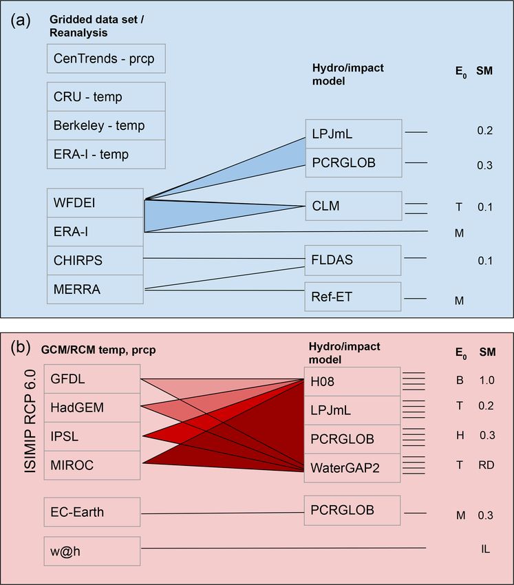
18                  S. F. Kew et al.: Impact of precipitation and increasing temperatures on drought trends in eastern Africa

1    Introduction                                                   moisture – because soil moisture is a better indicator of crop
                                                                    health than precipitation alone and it embodies the net effect
In eastern Africa, drought has occurred throughout known            of the supply and demand side of the water balance in regions
history with significant impacts on the agricultural sector and     without irrigation. Whilst short term single-season drought
the economy, particularly through threats to food security. It      episodes can be severe, we choose to analyse changes in
is therefore important to examine the role of anthropogenic         drought on annual rather than sub-annual timescales because
climate change in drought, particularly in the face of the          the worst crises in food security in this region have occurred
large-scale droughts of 2010/11, 2014, and 2015 in Ethiopia         with multiple-season droughts (Funk et al., 2015). We will
and the 2016/17 drought in Somalia, Kenya, and parts of             also investigate the influence of the main meteorological
Ethiopia and surrounding countries, which have raised the           drivers of soil moisture trends, i.e., precipitation and temper-
spectre of climate change as a risk multiplier in the region.       ature. Ideally, we would study the influence of temperature
   Droughts are triggered and maintained by a number of             on soil moisture via ET, however observational records are
factors and their interactions, including meteorological forc-      very limited in time and space and, as the spatial decorrela-
ings and variability, soil and vegetation feedbacks, and hu-        tion lengths of ET are short, their informational value is lim-
man factors such as agricultural practices and management           ited. We therefore analyse evaporative demand (E0 ; some-
choices, including irrigation and grazing density (van Loon         times also referred to as “potential evapotranspiration”, or
et al., 2016). Accordingly, there are several definitions of        PET, although this is strictly only one metric of E0 ). E0 is
drought in common use (Wilhite and Glantz, 1985): meteoro-          the amount of evaporation that would occur under prevail-
logical drought (precipitation deficit), hydrological drought       ing meteorological conditions if an unlimited supply of water
(low streamflow), agricultural drought (low soil moisture)          were available; in that sense, E0 measures the thirst of the at-
and socioeconomic drought (including water supply and de-           mosphere. E0 is calculable as a function of temperature, hu-
mand). This complexity of droughts poses challenges for             midity, solar radiation, and wind speed. We use a variety of
their attribution. It is not straightforward to disentangle these   common parameterizations of E0 that includes both potential
interacting factors, but over long periods it may be possible       evapotranspiration and reference evapotranspiration and that
to detect a climate change signal.                                  ranges in physical representation and complexity from sim-
   Previous attribution studies for eastern Africa have mainly      ple estimates based solely on temperature (the Hamon equa-
focussed on meteorological drought drivers (precipitation           tion), through estimates that also include solar radiation as a
deficit), with recent studies finding little or no change in the    driver (the Priestley–Taylor equation), and ultimately to fully
risk of low-precipitation periods due to anthropogenic cli-         physical estimates that further include humidity and wind
mate change (e.g., Philip et al., 2018a; Uhe et al., 2018).         speed as drivers (the Penman–Monteith equation). All nec-
Some weather stations in eastern Africa have recorded a de-         essary drivers are available for both observations and model
crease in precipitation in recent years; however, climate mod-      simulations. In this manner, we bracket the complexity in E0
els generally project an increase in mean precipitation but         parameterizations in a convergence-of-evidence approach fa-
give conflicting results for the probability of very dry rainy      miliar to the drought-monitoring community.
seasons (e.g., Shongwe et al., 2011). The reasons for the re-          We investigate E0 as a means to study the influence of
cent observed decrease in precipitation thus remain unclear,        temperature on soil moisture; however, for regions that are
but the trend is within the large observed natural variability      irrigated or where irrigation is being considered, E0 itself can
in the region, at least for the historical and current climate.     be regarded as more relevant than soil moisture as a measure
   However, precipitation only covers one aspect of drought –       of drought tendency.
that of the supply side of the water balance. The demand side          Whilst attribution studies specific to the eastern African
is represented by actual evapotranspiration (ET), which is          region have not previously used soil moisture or E0 to ex-
a function of moisture availability and evaporative demand.         plore drought, E0 has been used in various attribution or
With increasing temperatures, there is an a priori assumption       trend studies outside this region to explore, for example, the
that rising evaporative demand will increase the demand side        influence of climate change on the hydrologic cycle in China
of the water balance and, all else equal, droughts will become      (e.g., Yin et al., 2010; Li et al., 2014; Fan and Thomas, 2018),
more severe. However, this assumption is not based on analy-        trends and variability at sites in western Africa (Obada et al.,
ses, which motivates an objective study. In this study, we aim      2017), and compound events of low precipitation and high
to understand if, despite no evident trend in precipitation, in-    E0 in Europe (Manning et al., 2018).
creasing temperatures could be exacerbating drought.                   Summarizing, the objectives of this study are first to con-
   In the current study we wish to align our drought defini-        sider the attribution question “do increasing global tempera-
tion as closely as possible with the major human impact of          tures contribute to drier soils and thus exacerbate the risk of
drought – the threat to food security. Across eastern Africa,       agricultural drought (low soil moisture) in eastern Africa?”
the quality and quantity of food production for domestic con-       and second to investigate if global-warming driven trends in
sumption is intimately linked to agricultural conditions. We        precipitation or local temperature via E0 explain any emerg-
therefore use the agricultural definition of drought – low soil     ing trend in agricultural drought. Our approach to attribu-

Earth Syst. Dynam., 12, 17–35, 2021                                                     https://doi.org/10.5194/esd-12-17-2021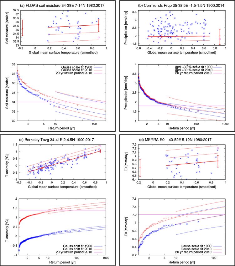
S. F. Kew et al.: Impact of precipitation and increasing temperatures on drought trends in eastern Africa 19
tion is comprised of the following steps: (1) definition of the for trend calculations and (ii) the model data pass the vali-
study variables and explanation of the study regions; (2) de- dation tests (see Sect. 3). For this purpose, we use time se-
scription of observational data and detection of trends in ob- ries of at least 35 years. As the focus of this paper is on an-
servations; (3) model evaluation including description of the nual timescales, using monthly data is sufficient. The obser-
models; (4) attribution of trends in models; and (5) synthesis vational and model datasets used in this study are shown in
of the results. Assessments will be based on both observa- Fig. 2 and listed in Tables 2 and 3 below (for brief descrip-
tions and climate and hydrological model output on an an- tions of the projects from which these data originate, see the
nual timescale, between the years 1900 (to represent the pre- Supplement.) Note that we use the data as they are available
industrial era) and 2018. We will illustrate the method using without applying any additional bias correction, resampling
examples of recent droughts in eastern Africa. or downscaling. Some of the data has undergone bias correc-
Section 2 of this paper presents the chosen study regions, tion within their projects of origin, as described in the Sup-
followed by a description of the datasets used in the study. plement.
Section 3 describes the stepwise approach to attribution used, The following subsections address the observational
including assumptions and decisions made and illustrative datasets and modelling datasets in turn.
examples. Section 4 synthesizes the results by region. Fi- Observational datasets. For observations of precipitation
nally, Sects. 5 and 6 present the discussion and conclusions. and daily mean near-surface temperature, we use gridded ob-
servational datasets and reanalyses.
For soil moisture and E0 , no direct observations meet-
2 Study variables, region, and datasets ing the above criteria exist. Instead, we use observational
estimates of soil moisture and E0 resulting from various
In this section, we present the chosen study variables and combinations of observational forcing data and models (see
study regions in eastern Africa and the datasets used to pro- Fig. 2a).
vide the variables to be analysed. Brief descriptions of the Observational series of soil moisture are few, generally too
projects from which the datasets originate are provided in short to use for trend analysis, and do not correlate well with
the Supplement. reanalysis or model data over eastern Africa (McNally et al.,
2016). It is therefore important to use multiple observation-
2.1 Study variables and region ally forced model estimates to span the large uncertainties
from inter-dataset differences. There being no a priori rea-
We analyse four different variables: soil moisture, precipita- son to favour one soil moisture dataset over another, we treat
tion, temperature, and E0 . We average these variables over all resulting soil moisture datasets equally. For both observed
six non-overlapping regions, as trend analyses of time series and modelled soil moisture datasets, we use the topmost layer
of regionally averaged quantities are more robust than the (see Fig. 2 for the depth of the topmost layer) provided by
same analyses for point locations. This is especially true for each dataset, except for the model weather@home where the
precipitation, which shows small-scale spatial variability if available soil moisture variable is an integrated measure of
the time period is not long enough to sufficiently sample the all four layers of soil moisture, including the deep soil. Each
distribution from multiple precipitation events. It is however time series is scaled to have a standard deviation of 1 in order
necessary to select homogeneous regions, so that the signals to make comparisons in trends possible.
present are not averaged out. E0 is a function of temperature, humidity, solar radiation,
The focus of the study is on eastern Africa – Ethiopia, and wind speed. Observational estimates of E0 used here
Kenya, and Somalia (including the Somaliland region). We originate from reanalysis datasets or reanalysis-driven im-
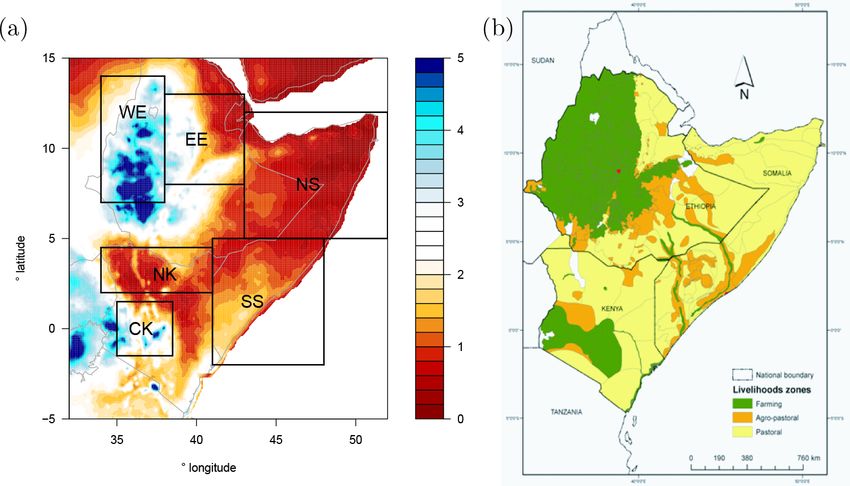
selected six regions based on precipitation zones in which pact models. For both observed and modelled E0 , there are
the annual mean precipitation and seasonal cycle are homo- various parameterizations, ranging from simple temperature-
geneous (Fig. 1a); livelihood zones (see Fig. 1b); and dis- or radiation-based schemes to sophisticated schemes based
cussions with local experts from the Kenya Meteorological on all the aforementioned components. Whilst the Penman–
Department, the National Meteorological Agency (NMA) of Monteith scheme is often considered superior (e.g., Hobbins
Ethiopia, and the Famine Early Warning Systems Network et al., 2016), one is often constrained from using a Penman–
(FEWS NET). The regions are shown in Fig. 1 and listed in Monteith parameterization due either to the lack of accurate
Table 1. Data are annually and spatially averaged over the or reliable input data or because the choice of E0 parameter-
study regions. ization within a given hydrological model setting is already
prescribed, as in the ISIMIP ensemble. We thus chose to use
2.2 Datasets a variety of E0 parameterizations (mostly the PET metric)
and input datasets in order to cover the range of possible E0
For the four study variables, we use all readily available values and trends in E0 . The E0 scheme used by each dataset
datasets over the study area, provided that (i) the data are is noted in Fig. 2.
sufficiently complete over a period long enough to be used
https://doi.org/10.5194/esd-12-17-2021 Earth Syst. Dynam., 12, 17–35, 202120 S. F. Kew et al.: Impact of precipitation and increasing temperatures on drought trends in eastern Africa
Table 1. The six study regions. See also Fig. 1.
Region Long name Latitude Longitude Months of seasonal Primary livelihood zone
precipitation peak(s)
WE Western Ethiopia 7–14◦ N 34–38◦ E Aug agropastoral/mixed land
EE Eastern Ethiopia 8–13◦ N 38–43◦ E Apr, Jul/Aug pastoral
NS Northern Somalia/Somaliland region 5–12◦ N 43–52◦ E Apr/May, Oct pastoral
and eastern Ethiopia
NK Northern Kenya 2–4.5◦ N 34–41◦ E Apr, Oct/Nov pastoral
CK Central Kenya 1.5◦ S–1.5◦ N 35–38.5◦ E Apr, Nov agropastoral/mixed land
SS Southern Somalia 2◦ S–5◦ N 41–48◦ E Apr/May, Oct/Nov pastoral/agropastoral
Figure 1. (a) Annual mean precipitation [mm/d] and the six study regions. Note that only land values are used. (b) Livelihood zones, which
were also used to define the study regions. Reprinted from Pricope et al. (2013) with permission from Elsevier.
Modelled datasets. Most simulations stem from the 3 Methods
ISIMIP project, which provides output of the variables un-
der investigation for four different impact models driven by In this section, we first describe the method for detection and
four different GCMs. These simulations are complemented attribution of trends in the four variables, including model
by other readily available model runs (EC-Earth-PCRGLOB- validation and the synthesis of observational and model re-
WB and weather@home) with different (but compatible) sults. Section 3.2 describes the assumptions and decisions
framings. that are made concerning the data and model setup, and
Using these various observations and modelled datasets, Sect. 3.3 provides an example of how the method is applied
we cover a wide range of different factors that influence to real data.
E0 and soil moisture. The different factors include meteo-
rological forcing, model choice, RCP scenario for the green- 3.1 Detection and attribution of trends
house gas concentration trajectory, E0 scheme, number of
soil layers and depth of topsoil layer, dynamic vegetation In this section we detect trends in observations and analyse
modelling (LPJmL only), and transient versus time-slice runs whether these trends, if present, can be attributed to human-
(see Sect. 3). induced climate change. In doing so, the approach taken to
communicating uncertainty is as follows.
– Perform a multi-model and multi-observation analysis
that summarizes what we currently know using readily
available data and methods.
Earth Syst. Dynam., 12, 17–35, 2021 https://doi.org/10.5194/esd-12-17-2021S. F. Kew et al.: Impact of precipitation and increasing temperatures on drought trends in eastern Africa 21
Table 2. Observational data used in this study.
Observational Full name Time period Spatial resolu- Citations(s)
dataset used tion (◦ lat ×
◦ long)
Observational/reanalysis dataset
CenTrends (prcp) Centennial Trends dataset 1900–2014 0.1 × 0.1 Funk et al. (2015)
CRU TS4 (temp) CRU TS4.01 1901–2018 0.5 × 0.5 Harris et al. (2014)
Berkeley (temp) Berkeley Earth 1900–2018 1.0 × 1.0 Rohde et al. (2013a, b)
ERA-I ERA-Interim 1979–2018 0.5 × 0.5 Dee et al. (2011)
Observation-driven hydro/impact model
LPJmL-WFDEI Lund-Potsdam-Jena managed 1971–2010 0.5 × 0.5 Bondeau et al. (2007); Rost
(soil moisture) Land – WATCH-Forcing-Data- et al. (2008); Schaphoff et al.
ERA-Interim (2013); Weedon et al. (2014)
PCRGLOB- PCRaster GLOBal Water Bal- 1971–2010 0.5 × 0.5 Sutanudjaja et al. (2018); Wee-
WFDEI (soil ance model – WATCH-Forcing- don et al. (2014)
moisture) Data-ERA-Interim
CLM-ERA-I (soil Community Land Model ver- 1979–2016 0.5 × 0.5 Oleson et al. (2010)
moisture, E0 ) sion 4 – ERA-Interim
CLM-WFDEI (soil Community Land Model 1979–2013 0.5 × 0.5 Lawrence et al. (2011); Weedon
moisture, E0 ) version 4 – WATCH-Forcing- et al. (2014)
Data-ERA-Interim
FLDAS (soil mois- Famine Early Warning Systems 1981–2018 0.1 × 0.1 McNally et al. (2017)
ture) Network (FEWS NET) Land
Data Assimilation System
MERRA Ref-ET Modern-Era Retrospective 1980–2018 0.125 × 0.125 Hobbins et al. (2018)
(E0 ) analysis for Research and
Applications Reference Evapo-
transpiration
– Apply simple evaluation techniques to readily avail- et al., 2018; Kew et al., 2019; Sippel et al., 2016), as it repre-
able data, treating datasets that satisfy evaluation cri- sents the current state of the art in extreme event attribution.
teria equally and rejecting the others. The method is extensively explained in van Oldenborgh et al.
(2021), Philip et al. (2020), van Oldenborgh et al. (2018), and
– Communicate uncertainties from synthesis. A simple
van der Wiel et al. (2017).
“yes” or “no” is not appropriate if there is no signifi-
In this study, for transient model runs and observational
cant trend. Instead, the uncertainties (confidence inter-
time series, we statistically model (i.e., fit) the dependency
vals) and their origin (e.g., natural variability or model
of annual means of the different variables on GMST (the
spread) are given.
model GMST for models and GISTEMP surface temperature
We use a multi-method, multi-model approach to address GMST (Hansen et al., 2010) for observations and reanalyses)
attribution. We use global mean surface temperature (GMST) as follows.
as a measure for anthropogenic climate change for calcu- After inspection of whether a Gaussian or a General Pareto
lating trends. We calculate trends for all variables, regions Distribution fits the observational and reanalysis data best,
and datasets and synthesize results into one overarching at- we use the following distributions.
tribution statement for each of the four variables (soil mois-
ture, precipitation, temperature, and E0 ) in each of the six – For soil moisture, a Gaussian distribution that scales
regions. We use this method, following the approach applied with GMST, focussing on low values.
in earlier studies on drought in eastern Africa (e.g., Philip
et al., 2018a; Uhe et al., 2018) and other drought- and heat- – For precipitation, a General Pareto Distribution (GPD)
attribution studies (e.g., Philip et al., 2018b; van Oldenborgh that scales with GMST, analysing low extremes.
https://doi.org/10.5194/esd-12-17-2021 Earth Syst. Dynam., 12, 17–35, 202122 S. F. Kew et al.: Impact of precipitation and increasing temperatures on drought trends in eastern Africa
Figure 2. Datasets used in this paper. (a) Observational precipitation (prcp) and near-surface temperature (temp) datasets and (b) models.
Listed under E0 is the E0 scheme (T: Priestley–Taylor; M: Penman–Monteith; H: Hamon; B: bulk formula) and under SM is the depth of the
top soil moisture layer available (RD: depends on rooting depth, 0.1–1.5 m for WaterGAP2; IL: integrated over all layers). Shading indicates
an experiment with either multiple input datasets or multiple hydrological models. The number of resulting hydrological model simulations
are indicated by horizontal lines on the right side of the figure.
– For temperature, a Gaussian distribution that shifts with with α in [units of the study variable]/K. When the distribu-
GMST, focussing on high values. tion is scaled,
µ = µ0 exp(αT /µ0 ), (2)
σ = σ0 exp(αT /µ0 ), (3)
– For E0 , a Gaussian distribution that scales with GMST,
which keeps the ratio of the location and scale parameter
focussing on high values.
σ/µ invariant. In each case, the fitted distribution is eval-
uated twice: once for the year 1900 and once for the year
2018. Confidence intervals (CI) are estimated using a non-
When the distribution is shifted, a linear trend α is fitted by parametric bootstrapping procedure. This allows us to cal-
making the location parameter µ dependent on GMST as culate the return period of an event as if it had happened in
the year 1900 or in the year 2018. To obtain a first-order ap-
proximation of the percentage change in the magnitude of the
µ = µ0 + αT , (1) study variable between the 2 reference years, α is multiplied
Earth Syst. Dynam., 12, 17–35, 2021 https://doi.org/10.5194/esd-12-17-2021S. F. Kew et al.: Impact of precipitation and increasing temperatures on drought trends in eastern Africa 23
Table 3. Model data used in this study.
Model dataset Full name Time period Spatial resolu- Citations(s)
used tion (◦ lat × ◦
long)
GCM/RCM
GFDL GFDL-ESM2M, Geophysical 1861–2018 2.02 × 2.5 Dunne et al. (2012, 2013)
Fluid Dynamics Laboratory –
Earth System Model 2M
HadGEM HadGEM2-ES, Hadley Centre 1859–2018 1.25 × 1.88 Collins et al. (2011); Jones et al.
Global Environmental Model (2011)
version 2-ES
IPSL IPSL-CM5A-LR, Institut Pierre 1850–2018 1.89 × 3.75 Dufresne et al. (2013)
Simon Laplace – CM5A-LR
MIROC MIROC5, Model for Interdisci- 1850–2018 1.4 × 1.4 Watanabe et al. (2010)
plinary Research on Climate –
version 5
EC-Earth EC-Earth 2.3 1850–2018 1.12 × 1.125 Hazeleger et al. (2012)
w@h (temp, prcp, soil Weather@home 2005–2016 and 0.11 × 0.11 Massey et al. (2015); Guillod
moisture) counterfactual et al. (2017)
climate
Hydro/impact models
H08 (soil moisture, E0 ) H08 1861–2018 0.5 × 0.5 Hanasaki et al. (2008a, b)
LPJmL (soil moisture, Lund-Potsdam-Jena managed 1861–2018 0.5 × 0.5 Bondeau et al. (2007); Rost
E0 ) Land model et al. (2008); Schaphoff et al.
(2013)
PCRGLOB (soil mois- PCRGLOB-WB, PCRaster 1861–2018 0.5 × 0.5 Sutanudjaja et al. (2018)
ture, E0 ) GLOBal Water Balance model
WaterGAP2 (soil mois- Water Global Analysis and 1861–2018 0.5 × 0.5 Müller Schmied et al. (2016)
ture, E0 ) Progress Model version 2
by 100 % times the change in GMST and divided by µ0 (for year 2018, i.e., in the current climate, is shown as a hori-
the shift fit this is exact). Note that for some variables – e.g., zontal line or square. Reading the return period at which this
precipitation – it is appropriate to scale rather than shift the line crosses the fit for the reference year 1900 shows how fre-
distribution with GMST (van Oldenborgh et al., 2021; Philip quent an event with a 20-year return period in today’s climate
et al., 2020). For the very large weather@home ensemble would have been at that time.
simulations of actual and counterfactual climates, it is not We only use results from model runs if they pass two dif-
necessary to use a fitting routine as the large amount of data ferent validation tests: a qualitative test on the seasonal cycle
permits a direct estimation of the trend. This also provides and a stronger test on variability. For soil moisture, due to
an opportunity to check the assumptions made in the fitting, the difficulties in obtaining reliable soil moisture measure-
notably that the values follow an extreme-value distribution ments (e.g., Liu and Mishra, 2017) and the differences be-
and that the distribution shifts or scales with the smoothed tween the observational (reanalysis) datasets, we cannot as-
GMST. We calculate trends for the time series of spatially sume that observational or reanalysis data are more accurate
and annually averaged data of all four variables and all six than model data. Therefore we simply use the soil moisture
regions for all datasets by dividing the difference in the vari- model data if the model input – precipitation and E0 – pass
able between the two ensembles by the difference in GMST. the validation tests.
Figures 3 and 4 present the methods applied to transient We perform only a qualitative validation of the seasonal
series and time slices, respectively. For reference and to aid cycle. For each region, each variable, and each model we
interpretation of the return-period diagrams, the magnitude check that the seasonal cycle resembles that of at least one of
of a hypothetical event with a 20-year return period in the the observational datasets, in terms of both the number and
https://doi.org/10.5194/esd-12-17-2021 Earth Syst. Dynam., 12, 17–35, 202124 S. F. Kew et al.: Impact of precipitation and increasing temperatures on drought trends in eastern Africa Figure 3. Illustrative examples of the fitting method for each variable for selected study regions: (a) FLDAS soil moisture (Gaussian fit, low extremes, region WE); (b) CenTrends precipitation (GPD fit, low extremes, region CK); (c) Berkeley temperature anomaly (Gaussian fit, high extremes, region NK); (d) MERRA E0 (Gaussian fit, high extremes, region NS). At the top of each panel the following information is given: annually averaged data (stars) against GMST and fit lines – the location parameter µ (thick), µ ± σ and µ ± 2σ (thin lines, Gaussian fits) and the 6- and 40-year return values (thin lines, GPD fit). Vertical bars indicate the 95 % confidence interval on the location parameter µ at the 2 reference years 2018 and 1900. The magenta square illustrates the magnitude of an event constructed to have a 20-year return period in 2018 (not included in the fit). At the bottom of each panel the following information is given: return period diagrams for the fitted distribution and 95 % confidence intervals, for the reference years 2018 (red lines) and 1900 (blue lines). The annually averaged data is plotted twice, being shifted or scaled with smoothed global mean temperature up to 2018 (red stars) and down to 1900 (blue stars). The magenta line illustrates the magnitude of a hypothetical event with a 20-year return period in 2018. the timing of peaks. If the seasonal cycle is very different, we still use the time series in soil moisture) and for temperature do not use the time series for that specific combination. This in region SS for EC-Earth (we do not have adjusted data to is the case for the original GCM precipitation in region NK check, so we do not use this model–region combination for for weather@home and in regions NK and CK for MIROC soil moisture or E0 ). (the seasonal cycle is improved in the adjusted dataset, so we Earth Syst. Dynam., 12, 17–35, 2021 https://doi.org/10.5194/esd-12-17-2021
S. F. Kew et al.: Impact of precipitation and increasing temperatures on drought trends in eastern Africa                                   25

Figure 4. Illustrative examples of the weather@home time slice model runs. (a) Annual mean precipitation [mm/d] in region WE. (b) Annual
mean temperature [◦ C] in region CK. The red markers are for the present-day climate and the blue markers are for the climate in pre-industrial
times. The magenta line illustrates the magnitude of a hypothetical event with a 20-year return period in the present-day climate.

   The second validation test is on the model variability in              ratios, because we can derive finite ranges in confidence in-
precipitation and E0 (variability relative to the mean for vari-          tervals for all variables. This is not the case for the proba-
ables that scale with GMST). If the model variability of a                bility ratio, where, for example, strong trends in temperature
specific variable in a specific region is outside the range of            imply that mild extremes of the 2018 climate (e.g., a 1-in-20-
variability calculated from observations or reanalyses, we do             year event) would have had a chance of almost zero around
not use that specific dataset for that specific region and vari-          1900, resulting in very large probability ratios and extensive
able. For temperature, we relax the validation criteria on vari-          extrapolation of the fit beyond the length of the dataset.
ability as it became clear during the analysis that the trend in             We synthesize the trends of all data that pass the valida-
soil moisture does not depend strongly on temperature and                 tion tests in the following manner (see also Fig. 5). The ob-
the trend in temperature agrees between models and obser-                 servational (reanalysis) estimates are based on the same nat-
vations. In two of the regions a strict validation resulted in            ural variability: the historical weather. They also cover sim-
only two driving GCMs. Trends from the resulting time se-                 ilar time periods. The uncertainties due to natural variability
ries that passed the validation tests are shown in Sect. 4 and            (denoted as solid blue in the synthesis figures) are therefore
in the figures in the Supplement.                                         highly correlated. We approximate these correlations by as-
   Using the large weather@home ensemble (which requires                  suming the natural variability to be completely correlated and
no fitting), we check the assumption that annual soil moisture            compute the mean and uncertainties as the average of the dif-
and precipitation scale with GMST and temperature shifts                  ferent observational estimates. The spread of the estimates is
with GMST. For E0 , we assume that the distribution scales                a measure of the representation uncertainty in the observa-
with GMST. In the weather@home ensemble, dry extremes                     tional estimate and is added as an independent uncertainty to
show less change than intermediate dry extremes, which sup-               the natural variability (outlined black boxes). This results in
ports our assumption that scaling with GMST is appropri-                  a consolidated value for the observations (reanalyses) drawn
ate (except for the higher return values, where the uncertain-            in dark blue.
ties are large). For soil moisture it is very difficult to distin-           In contrast, model estimates have more uncorrelated nat-
guish between scaling and shifting from the weather@home                  ural variability: totally uncorrelated for coupled models and
ensemble because the trend is small. For temperature the                  largely uncorrelated for SST-forced models (the predictabil-
weather@home ensembles indicate that the highest temper-                  ity of annual mean precipitation given perfect SSTs is low
atures are increasing slower than the lower temperatures.                 in eastern Africa). We approximate these correlations by tak-
This implies that the variability decreases with GMST; how-               ing the natural variability to be uncorrelated. The spread of
ever, no consistent signal in the observations or other models            model results can be compared by the spread expected by the
is evident (we see a small increase in variability with time              natural variability by computing the χ 2 /dof statistic. If this is
for Berkeley, a small decrease for CRU, and no consistency                greater than one, there is a noticeable model spread, which is
between the models). This does not significantly affect the               added in quadrature to the natural variability. This is denoted
trend, which is evaluated for the centre of the distribution.             by the white boxes in Fig. 5. The bright red bar indicates
   Trends are presented as change in a variable per degree                the total uncertainty of the models, consisting of a weighted
of GMST warming. We show trends rather than probability                   mean using the (uncorrelated) uncertainties due to natural

https://doi.org/10.5194/esd-12-17-2021                                                            Earth Syst. Dynam., 12, 17–35, 2021
26                  S. F. Kew et al.: Impact of precipitation and increasing temperatures on drought trends in eastern Africa

Figure 5. Illustrative examples of the synthesized values of trends per 1 K GMST rise for soil moisture [/K] (a), precipitation [mm/d/K] (b),
temperature [K/K] (c), and E0 [mm/d/K] (d) for region SS. Black bars are the average trends, coloured boxes denote the 95 % CI. Blue
represents observations and reanalyses, red represents models, and magenta represents the weighted synthesis. Coloured bars denote natural
variability, and white boxes also take representativity and model errors into account, if applicable (see Sect. 3). In the synthesis, the magenta
bar denotes the weighted average of observations and models and the white box denotes the unweighted average. Soil moisture trends are
based on standardized data; the other trends are absolute trends.

variability plus an independent common model spread added                  servations. This is indicated by the white box around the ma-
to the uncertainty in the weighted mean.                                   genta bar. Whichever type of weighting is chosen, both the
   Finally, observations and models are combined into a sin-               best estimate and uncertainty ranges are communicated.
gle result in two ways. Firstly, we compute the weighted av-
erage of the synthesized values for models and observations,               3.2   Assumptions and decisions
neglecting model uncertainties beyond the model spread: this
is indicated by the magenta bar. However, we know that mod-                We made the following assumptions and decisions about the
els in general struggle to represent the climate of eastern                data and model setup in addition to completing the model
Africa, so the model uncertainty is larger than the model                  evaluation to attain data of sufficient quality.
spread. Therefore, we also use the more conservative esti-
mate of an unweighted average of the synthesized values for                  1. The CenTrends precipitation dataset includes many dif-
observations and models, which gives more weight to the ob-                     ferent sources of precipitation data and more stations
                                                                                than most other datasets (Funk et al., 2015). We there-

Earth Syst. Dynam., 12, 17–35, 2021                                                              https://doi.org/10.5194/esd-12-17-2021
S. F. Kew et al.: Impact of precipitation and increasing temperatures on drought trends in eastern Africa 27
fore assume it to be superior relative to other datasets 7. We focus on the historical time frame. Therefore the
over our study region; it is therefore our only source of trends in different RCP and socio-economic scenarios
observations of precipitation. will be relatively similar to each other. The forcing data
is the same for the years 1860–2005 and only differs for
2. In general, we use the longest time series of data avail- the most recent years from 2006 onwards. In general,
able. We make exceptions in the starting year based on however, using different scenarios can be seen as an ad-
visual inspection of abrupt changes due to data limita- vantage, as a greater range of scenario uncertainty will
tions toward the beginning of the time series. be spanned.
a. We use Berkeley starting from 1900, except in re-
gion SS, where we start in 1920. a. We use RCP6.0 in ISIMIP as this choice resulted
in the largest number of simulations and RCP8.5 in
b. We use CRU starting from 1901, except in regions EC-Earth as this was the only scenario available.
NK, CK, and SS, where we start in 1940.
b. We selected the “historical” socio-economic sce-
3. Across our study region, no realistic soil moisture nario in ISIMIP model runs for 1860–2005 and
dataset exists covering a long-enough time period to cal- “2005soc” for 2006–present; for H08, historical
culate trends. Therefore we do not select simulations was unavailable for years 1860–2005, so we instead
based on evaluation criteria other than selecting runs used 2005soc for those years and for years 2006–
based on precipitation and E0 evaluation in the input present. For the WFDEI experiments, 2005soc was
variables. unavailable, so we used historical before 2006 and
4. As models do not share a consistent set of soil moisture “varsoc” for the years 2006–2018.
levels, we take the top level of each model, assuming
8. Trends are calculated or extrapolated using all data up to
that this is the most comparable level across models. We
2018 and between the pre-industrial era (1900) and the
checked for LPJmL – the only selected ISIMIP hydro-
present (2018). Weather@home is an exception, where
logical model that has more than one level available for
trends are calculated between two stationary climates
soil moisture – that the variability does not change sig-
of the present and the pre-industrial era. Differences in
nificantly when integrating over multiple levels instead
trends can arise due to different time periods and lengths
of using level 1.
of datasets, which are generally shorter for observa-
5. Within the ISIMIP project, variables required by the hy- tional series and reanalyses than for model simulations.
drological models, including precipitation and tempera- However, we consider the use of all available observa-
ture, were bias-corrected and the adjusted data was used tional and reanalysis data and different model framings
to calculate E0 and to drive the hydrological models to lead to a more complete and robust attribution state-
to output soil moisture. In the synthesis, however, we ment.
present results for precipitation and temperature based
on the unadjusted data, on the principle that this better 9. We analyse January–December annual means. Based on
spans the range of model uncertainty in these variables. the seasonal cycles of precipitation and temperature, for
The bias correction applied in ISIMIP aims to conserve all regions except for the region WE (which has a sin-
the original trend (Hempel et al., 2013). Therefore, we gle rainy season) we could also have chosen to analyse
find little change in trend for most time series. July–June annual means instead. The influence of this
choice on the trends is low (see also Sect. 3.3).
6. In using our variety of E0 metrics, we do not convert ref-
erence evapotranspiration (such as that drawn from the 10. For consistency in the method, we fit the variability as
MERRA-2 dataset (Hobbins et al., 2018) to PET, nor a constant over time for all data. In both observed time
do we use crop coefficients to convert reference evap- series and simulations we see very little or no trend in
otranspiration to crop evapotranspiration because do- variability up to 2018.
ing so would not be relevant to the research purposes.
Our study is only interested in evaporative demand in 11. If for observational data a Gaussian fit is the best fit, we
its purest sense – i.e., as the atmospheric control driving also fit model data to a Gaussian, even if a GPD is a bet-
upward moisture flux in the land–atmosphere system. In ter fit for that data. In doing this we avoid erroneous
any case, crop coefficients we used would be (i) so in- comparisons between the variable mean and variable
accurate as to be meaningless at the large spatial scales extreme. We checked for model runs in which this dis-
of our analysis and (ii) different for each of the different parity occurs but found that in most cases the trend cal-
metrics of E0 that we use. The ensemble of E0 values culated from fitting model data to a GPD was not very
generated by our variety of E0 metrics will ensure that different from the trend calculated from fitting model
significant trends generated are robust. data to a Gaussian.
https://doi.org/10.5194/esd-12-17-2021 Earth Syst. Dynam., 12, 17–35, 202128 S. F. Kew et al.: Impact of precipitation and increasing temperatures on drought trends in eastern Africa
3.3 Illustrative examples
In this section we show an example to illustrate the method
of detection of trends in precipitation data, as drought is of-
ten experienced as reduced or failed rainy seasons. For this
purpose, we calculated return periods and risk ratios of re-
cent droughts defined as low-precipitation events on an an-
nual timescale (see Table 4). Note that the risk ratios are
calculated from CenTrends alone and are not synthesized
values based on a multi-model analysis. The synthesis of
observations with models follows in the next section. We
chose events based on the Emergency Events Database (EM-
DAT) – an extensive global database of the occurrence of,
and effects incurred from, extreme weather events – and
the time series calculated from CenTrends (up to Decem-
ber 2014 only, which excludes the recent droughts of 2015
and 2016/2017). For the three northern study regions (WE,
EE, and NS) we chose the year 2009, in which the first rainy
season failed (in region WE, where there is only one peak
in precipitation, the whole season had slightly lower precip-
itation amounts). For the southern three study regions (CK,
NK, and NS) we choose the year 2005, in which the sec-
ond rainy season failed. Additionally, we also investigated
the well-known 2010/2011 drought for the regions NK and
SS. As this drought occurred from late 2010 to early 2011
(the second part of 2011 was in fact very wet), we define the
annual period of this specific 2010/2011 analysis to be July–
June.
Taking region WE as an example, the results show that in
CenTrends the trend in precipitation between 1900 and 2018
is −0.09 mm/d/K (95 % CI −0.51 to 0.14 mm/d/K). With a
change in GMST of 1.07 K and a mean precipitation in 1900
of 3.2 mm/d, this is similar to a change of 3 %. Thus, if an Figure 6. Summary of the synthesized values for (a) soil moisture
event with the same precipitation amount as in the year 2009 in [/K], (b) precipitation in [mm/d/K], (c) temperature in [K/K], and
had happened again in 2018 it would have been a 1-in-30- (d) E0 in [mm/d/K] in the six regions. The magenta bars denote the
year event (95 % CI 2 to 400) in 2018, whereas in 1900 it weighted averages of observations and models, and the white boxes
would have been a 1-in-80-year event (95 % CI 30 to 1400), denote the unweighted averages.
corresponding to a probability ratio of 2.5 (95 % CI 0.2 to
380). A return period that decreases in time indicates that
such extreme droughts are becoming slightly more common; diate synthesis figures of all six regions can be found in the
however, in this example we see large uncertainties consis- Supplement. Table 5 and Fig. 6 summarize final synthesized
tent with no change. Note that the trend and probability ratio findings for all regions. Using both the intermediate and final
are not significantly different from zero at p < 0.05. The re- synthesis results, we first draw conclusions based on different
sults for all regions are summarized in Table 4. (We note that GCMs and hydrological models and then turn to conclusions
the trends calculated for the January–December events and for each variable.
for the July–June events in regions NK and SS respectively First, we look for consistent behaviour in the trends from
are not significantly different. This supports the decision to individual GCMs across the four variables. We note that the
analyse January–December annual extremes only.) results from low-resolution GCMs do not consistently stand
out compared to higher-resolution models and also over-
4 Synthesis results lap with observational uncertainty. Some general conclusions
about the different GCMs are as follows: (i) for GCM-driven
In this section, we illustrate the synthesis method. Interme- model runs with stronger positive trends in temperature, there
diate synthesis figures, which show not only the overall syn- is a tendency for the positive trends in E0 also to be stronger
thesis but also the results for individual models, are presented and vice versa for weaker trends; (ii) the uncertainty in pre-
for the region SS for each of the four variables; the interme- cipitation trends is high compared to the trend magnitudes,
Earth Syst. Dynam., 12, 17–35, 2021 https://doi.org/10.5194/esd-12-17-2021S. F. Kew et al.: Impact of precipitation and increasing temperatures on drought trends in eastern Africa 29
Table 4. Trends, return periods, and probability ratios of equivalent events in the year 2018 and 1900 for three recent drought events registered
in the EM-dat database (2005, 2009, and 2010/2011), based on annual average precipitation (mm/d) from the CenTrends dataset. The 95 %
confidence intervals are given between brackets. For each study region impacted by the events, the annual precipitation for the event year
(Prcp, used to define the event magnitude) and the 1900–2014 climatological precipitation average (ClimPrcp) is given. The asterisk ∗ denotes
that July–June is taken instead of January–December to define a year.
Region Event year Prcp ClimPrcp Trend [mm/d/K] Return period in Return period in Probability ratio
1900–2014 2018 1900
WE 2009 2.94 3.38 −0.09 (−0.51 to 0.14) 30 (2 to 400) 80 (30 to 1400) 2.5 (0.2 to 380)
EE 2009 1.49 1.84 −0.03 (−0.35 to 0.07) 40 (3 to 340) 50 (25 to 560) 1.4 (0.4 to 70)
NS 2009 0.42 0.63 0.07 (−0.08 to 0.12) 80 (4 to 300) 10 (5 to 46) 0.13 (0.03 to 6.7)
NK 2005 0.77 1.10 −0.07 (−0.26 to 0.12) 5 (2 to 30) 10 (5 to 22) 1.9 (0.3 to 6.5)
CK 2005 1.75 2.39 0.04 (−0.55 to 0.43) 29 (3 to 200) 22 (12 to 63) 0.77 (0.11 to 14)
SS 2005 0.74 1.09 0.03 (−0.12 to 0.22) 29 (4 to 470) 17 (6 to 47) 0.61 (0.02 to 7.80)
CK 2010/2011∗ 0.51 1.10 0.16 (−0.30 to 0.27) 650 (10 to 20 000) 130 (53 to 2200) 0.21 (0.03 to 64)
SS 2010/2011∗ 0.53 1.09 0.02 (−0.31 to 0.21) 300 (12 to 40 000) 230 (90 to 8100) 0.77 (0.03 to 80)
Table 5. Summary of synthesis results for each region and study For soil moisture we find no significant synthesized trends:
variable. Note that “0” means no significant change, a “+” sign in- there is practically no change in region EE and no trend to a
dicates a positive trend, and a “−” sign indicates a negative trend. small, positive but non-significant trend in regions WE, NS,
The uncertainties associated with each result are depicted in Fig. 6. NK, CK and SS.
For precipitation, regions WE and NK show a positive
Region Soil Precipitation Temperature E0 but non-significant trend, although in region WE models and
moisture observations only partially overlap. In region NS there is a
WE 0/+ 0/+ + + small positive trend, regions EE and CK show no trend (for
EE 0 0 + + EE only with partial overlap of models and observations),
NS 0/+ + + + and region SS shows a negative, non-significant trend.
NK 0/+ 0/+ + 0/+ As expected from global climate change, the local an-
CK 0/+ 0 + 0/+ nually averaged temperatures all have a significant positive
SS 0/+ 0/− + + trend, with best estimates between 1.0 and 1.3◦ per degree of
GMST increase. Related to this, trends in E0 are also posi-
tive in four of the six regions but lower than for temperature
which partially explains why a clear relation with soil mois- and generally have larger confidence intervals. The regions
ture trends is not evident; and (iii) no clear relation between NK and CK are the exceptions. Although weighted averages
local temperature trends and soil moisture trends is evident. show positive trends, models show tendencies opposite to the
Looking at the different hydrological models, we conclude observations. This incompatibility renders the results uncer-
that the trend in PCR-GLOBWB E0 , which uses the Hamon tain.
E0 scheme that depends only on temperature, is generally We can identify the following relationships between differ-
higher than the trend in EC-Earth E0 , which uses the more ent variables: (i) precipitation trends have a (small) influence
complex Penman–Monteith E0 scheme that additionally de- on soil moisture trends in regions WE, NS, and NK; (ii) in
pends on humidity, wind speed, and solar radiation. Using regions WE, EE, NS, NK, and CK, temperature and E0 have
this more complex scheme can influence the trend in soil no discernible influence on soil moisture trends; (iii) in re-
moisture, especially in wetter regions. gion SS, the non-significant negative trend in precipitation
The analyses of the individual model runs, stratifying by does not lead to lower soil moisture and neither do the trends
GCM or hydrological model, do not lead to a clear conclu- in temperature or E0 . While it would be desirable to link the
sion on the relation between the trends in soil moisture, pre- overall findings to differences in regional climate, the dif-
cipitation, temperature, and E0 . We therefore turn to the anal- ferences in the synthesized results between regions are too
ysis of the synthesized values (see Table 5 and Fig. 6 for a small relative to confidence intervals to be able to say any-
summary of the outcome and Figs. 5 and S1 to S6 in the thing meaningful. It was nevertheless necessary to divide the
Supplement for synthesis diagrams). Table 5 summarizes the study area into homogeneous regions, so that extremes expe-
interpretation of the synthesized results shown in Fig. 6. The rienced within each region are representative for that region
more the magenta bar is centred in the white box, the better and inhomogeneity is not influencing the location of the oc-
the models agree with observations and the more we trust our currence of extremes.
attribution statement.
https://doi.org/10.5194/esd-12-17-2021 Earth Syst. Dynam., 12, 17–35, 202130 S. F. Kew et al.: Impact of precipitation and increasing temperatures on drought trends in eastern Africa
5 Discussion sites in Europe. They found that at water-limited sites the in-
fluence of precipitation on soil moisture is much larger than
In this section, we interpret our results in the light of how our that of temperature via E0 . In our study, we find the same
choices and assumptions may have influenced the outcomes for the driest regions and the driest months in the wetter re-
and we compare them to previous studies. gions, and for the more temperature-based E0 schemes. This
Whilst it may be preferable to use soil moisture as a is presumably because temperature-based schemes (such as
drought indicator, observations and simulations of precipi- the Hamon approach) do not reflect land surface–atmosphere
tation are more reliable in this region (Coughlan de Perez interactions as well as those that are also driven by humidity
et al., 2019). Precipitation has a large influence on agricul- and wind speed (such as the Penman–Monteith approach) or,
tural droughts and is therefore appropriate to use in attri- to a lesser degree, by radiation (such as the Priestley–Taylor
bution studies in eastern Africa, supplementing the analy- approach).
sis of soil moisture. The outcome of previous studies that Previous studies have shown that both the E0 scheme
have focussed on precipitation deficits only (e.g., Philip et al., and their input data can have a large influence on E0 val-
2018a; Uhe et al., 2018) are thus still relevant and compare ues (Trambauer et al., 2014; Wartenburger et al., 2018).
well with our results, i.e., that no consistent significant trends We confirm this using the CLM-ERA-PT (Priestley–Taylor),
in droughts are found. A comparison between seasonal cy- CLM-WFDEI-PT, and CLM-ERA-PM (Penman-Monteith)
cles of the different variables (averaging the monthly means datasets (not shown). In our study regions, E0 values are con-
over recent decades) shows that the seasonal cycle of soil sistently higher when using PM than when using PT. The dif-
moisture is similar to that of precipitation in all six study re- ferences in trends in E0 using ERA or WFDEI input or using
gions. In contrast, the inverse seasonal cycle of temperature PT or PM input are sometimes significant. However, compar-
is not similar to that of soil moisture. Whether the E0 sea- ing study regions, there is no consistency in the difference; in
sonal cycle reflects elements of the soil moisture cycle or not four out of the six regions the PM data shows a higher trend
depends on the E0 scheme used: temperature- or radiation- than the PT data, and in four out of the six regions WFDEI
based schemes show a seasonal cycle that is similar to that of data shows a higher trend than the ERA data.
temperature, whereas more advanced schemes reflect a mix- A study by Rowell et al. (2015) discussed the possibility
ture between the seasonal cycles of precipitation and temper- that climate model precipitation trends in East Africa are in-
ature, as they also synthesize the seasonal cycle in humidity, fluenced by the inability of the models to reliably represent
which is strongly correlated to that of precipitation. We thus key physical processes. Rainy seasons in this region are gov-
conclude that the influence of precipitation on soil moisture erned by large-scale processes, such as El Niño-Southern Os-
is higher than that of temperature or most E0 schemes. This cillation (ENSO) dynamics and the shifting of the Intertrop-
is supported by the synthesized results that show negligible ical Convergence Zone (ITCZ). We view the tests we per-
or no trends in soil moisture and precipitation, whereas the form on seasonal cycle and frequency distributions, which
trends in temperature and E0 are strongly positive. provide some assurance that large-scale physical processes
If temperature has an influence on trends in soil moisture are reasonably well described, to be a minimum requirement
(through E0 ), we expect to see that the positive trend in tem- for model validation. To improve the performance of mod-
perature is coupled to a drying soil moisture trend. As we els and to understand the discrepancies between models and
average over the annual scale, we may miss parts of the sea- observations, a much more thorough investigation into the
son when this effect is strongest. Therefore, we selected a models’ representation of physical processes and feedbacks
region and period outside the rainy season in which the sea- is required, such as demonstrated by James et al. (2018) and
sonal peak in temperature corresponds to a dip in soil mois- encouraged by the IMPALA (Improving Model Processes
ture (region CK, months February–March) to inspect sub- for African Climate) project (https://futureclimateafrica.org/
annual trends (not shown). Even then, we find that there is project/impala/, last access: last access: 9 November 2018).
no negative trend in soil moisture accompanying the positive In the long term, a trend in E0 only has meaning for
temperature trends. crop growth if there is water available for evapotranspira-
We study drought trends on annual as opposed to sub- tion. Much of eastern Africa is in a water-limited hydrocli-
annual timescales, as long-term drought presents a greater mate, requiring irrigation for crop growth. In irrigated ar-
risk for food security. On the annual timescale, we do not eas within larger water-limited regions, the increased wa-
see strong explanatory relationships between the trends in the ter availability shifts the local hydroclimate away from the
four studied variables (soil moisture, precipitation, tempera- surrounding water-limited regime towards a locally energy-
ture, and E0 ). To gain insight into the relationships between limited regime. Positive trends in E0 seen in our analyses (es-
the variables, we additionally looked at correlations on a pecially if the variety of different schemes produces a robust
sub-annual timescale. Simple correlations between monthly E0 trend) could then signify a trend in actual ET and would
soil moisture, precipitation, temperature, and E0 (not shown) therefore be accompanied by an increase in both irrigation
support the conclusions of Manning et al. (2018) on the influ- water demand and, if that demand can be met, in crop growth.
ence of precipitation and E0 on soil moisture at water limited However, it should be noted that irrigation is not accounted
Earth Syst. Dynam., 12, 17–35, 2021 https://doi.org/10.5194/esd-12-17-2021You can also read