Intercomparison of cosmic-ray neutron sensors and water balance monitoring in an urban environment - GI
←
→
Page content transcription
If your browser does not render page correctly, please read the page content below
Geosci. Instrum. Method. Data Syst., 7, 83–99, 2018
https://doi.org/10.5194/gi-7-83-2018
© Author(s) 2018. This work is distributed under
the Creative Commons Attribution 3.0 License.

Intercomparison of cosmic-ray neutron sensors and water balance
monitoring in an urban environment
Martin Schrön1 , Steffen Zacharias1 , Gary Womack2 , Markus Köhli1,3,4 , Darin Desilets2 , Sascha E. Oswald5 ,
Jan Bumberger1 , Hannes Mollenhauer1 , Simon Kögler1 , Paul Remmler1 , Mandy Kasner1,6 , Astrid Denk1,7 , and
Peter Dietrich1
1 Dep.  Monitoring and Exploration Technologies, Helmholtz Centre for Environmental Research GmbH – UFZ,
Leipzig, Germany
2 Hydroinnova LLC, Albuquerque, USA
3 Physikalisches Institut, Heidelberg University, Heidelberg, Germany
4 Physikalisches Institut, University of Bonn, Bonn, Germany
5 Institute of Earth and Environmental Science, University of Potsdam, Potsdam, Germany
6 Institute of Geosciences and Geography, University of Halle-Wittenberg, Halle, Germany
7 Dep. of Geosciences, University of Tübingen, Tübingen, Germany

Correspondence: Martin Schrön (martin.schroen@ufz.de)

Received: 13 May 2017 – Discussion started: 7 July 2017
Revised: 27 January 2018 – Accepted: 3 February 2018 – Published: 9 March 2018

Abstract. Sensor-to-sensor variability is a source of error      area (25 ha) have revealed substantial sub-footprint hetero-
common to all geoscientific instruments that needs to be         geneity to which CRNS detectors are sensitive despite their
assessed before comparative and applied research can be          large averaging volume. The sealed and constantly dry struc-
performed with multiple sensors. Consistency among sen-          tures in the footprint furthermore damped the dynamics of
sor systems is especially critical when subtle features of the   the CRNS-derived soil moisture. We developed strategies to
surrounding terrain are to be identified. Cosmic-ray neutron     correct for the sealed-area effect based on theoretical insights
sensors (CRNSs) are a recent technology used to monitor          about the spatial sensitivity of the sensor. This procedure not
hectometre-scale environmental water storages, for which a       only led to reliable soil moisture estimation during dry-out
rigorous comparison study of numerous co-located sensors         periods, it further revealed a strong signal of intercepted wa-
has not yet been performed. In this work, nine stationary        ter that emerged over the sealed surfaces during rain events.
CRNS probes of type “CRS1000” were installed in rela-            The presented arrangement offered a unique opportunity to
tive proximity on a grass patch surrounded by trees, build-      demonstrate the CRNS performance in complex terrain, and
ings, and sealed areas. While the dynamics of the neutron        the results indicated great potential for further applications in
count rates were found to be similar, offsets of a few percent   urban climate research.
from the absolute average neutron count rates were found.
Technical adjustments of the individual detection parameters
brought all instruments into good agreement. Furthermore,
we found a critical integration time of 6 h above which all      1   Introduction
sensors showed consistent dynamics in the data and their
RMSE fell below 1 % of gravimetric water content. The            The monitoring of water states and fluxes is important to
residual differences between the nine signals indicated local    understand processes of the hydrological cycle, to facilitate
effects of the complex urban terrain on the scale of several     weather predictions, and to make timely decisions (Wood
metres. Mobile CRNS measurements and spatial simulations         et al., 2011; Beven and Cloke, 2012). Soil moisture and
with the URANOS neutron transport code in the surrounding        air humidity are interlinked key quantities that can control
                                                                 plant water availability, groundwater recharge, air temper-

Published by Copernicus Publications on behalf of the European Geosciences Union.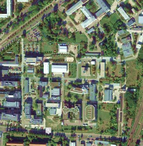
84                             M. Schrön et al.: Intercomparison of cosmic-ray neutron sensors in an urban environment

ature, and regional weather phenomena (Seneviratne et al.,         ple, Chiba et al. (1975) and Oh et al. (2013) revealed clear
2010). In urban environments, sealed surfaces reduce water         discrepancies between high-energy neutron monitors which
infiltration and promote high evaporation from ponded wa-          were related to device-specific configurations. Intercalibra-
ter. These effects are linked with the formation and impact        tion may be employed to normalize such differences from
of urban heat islands and can be a major threat for society        unit to unit and also to account for any residual instrumental
(Arnfield, 2003; Starke et al., 2010; UN, 2015).                   configuration inconsistencies (Bachelet et al., 1965; Krüger
    Conventional measurement methods for soil and evapora-         et al., 2008).
tion water operate on a point scale and are not representa-           When it comes to data analysis and interpretation, spatial
tive of complex areas (Famiglietti et al., 2008; Schelle et al.,   heterogeneity could have a biasing effect on neutron detec-
2013), while remote-sensing products are often limited to          tors. Despite the large footprint, the sensor is not equally
low resolution and shallow penetration depth (Nouri et al.,        sensitive to every part. Its radial sensitivity decreases non-
2013; Fang and Lakshmi, 2014). Up to now, few methods              linearly with distance, showing pronounced sensitivity to the
have been available to assess the components of the hydro-         nearest few metres around the probe (Köhli et al., 2015). This
logical cycle non-invasively and on relevant scales (Robinson      might become a particular issue for co-located sensors dur-
et al., 2008).                                                     ing an intercomparison study and for the reliability of soil
    The method of cosmic-ray neutron sensing (CRNS) com-           moisture estimations in complex terrain (Franz et al., 2013;
bines the geoscientific research fields of cosmic-ray neutron      Schrön et al., 2017a). Nonetheless, researchers have chal-
detection and environmental hydrology (Desilets et al., 2010;      lenged the task to interpret CRNS data in complex environ-
Zreda et al., 2012). The instrument is an epithermal neutron       ments (Bogena et al., 2013; Franz et al., 2016; Schattan et al.,
detector that measures the natural cosmic-ray-induced radi-        2017; Schrön et al., 2017b), but open questions remain of
ation 1–2 m above the ground and is highly sensitive to the        how and to what degree spatial heterogeneity should be ac-
abundance of hydrogen atoms in the surrounding area. As            counted for.
neutrons can penetrate the soil up to depths of approximately         The CRNS measurements come with an intrinsic statis-
80 cm and are then able to travel several hundreds of me-          tical uncertainty which is higher for lower count rates and
tres in air, the unique feature of the technology is the large     decreases with longer integration time. Among others, Evans
averaging volume (Köhli et al., 2015). The CRNS research           et al. (2016) and Hawdon et al. (2014) reported issues with
field aims to fill the gap between point-scale and large-scale     low hourly count rates in wet regions and at low altitude.
measurements by using the sensor in a stationary and mobile        Bogena et al. (2013) found that the error in volumetric soil
mode. The main advantages of the method are its capabil-           moisture estimates can be 10–20 % for hourly CRNS data in
ities to capture different components of the water cycle in        a forested environment. This statistical noise might become
air, soil, and vegetation non-invasively (e.g. Baroni and Os-      a problem for the reliability and consistency of CRNS mea-
wald, 2015) and to provide a representative spatial average        surements.
of the environmental water content. Therefore, the method is          The main objective of this paper is to advance the gener-
a promising candidate to support hydrogeophysical and cli-         ation of reliable CRNS products. To achieve this, we aim to
mate research in complex terrain (e.g. urban environments).        explore the potential sensor-to-sensor variability of cosmic-
    Consistency among the neutron signals is an important          ray neutron sensors in a systematic way and to provide so-
prerequisite towards joint usage of multiple sensors for           lutions to improve the consistency of neutron measurements.
scientific applications. Many studies relied on the consis-        With regards to the potential sources of variability in the neu-
tent performance of a set of CRNS probes for monitor-              tron signal, we can formulate the following hypotheses:
ing (Rivera Villarreyes et al., 2011; Dong et al., 2014;
Franz et al., 2015; Evans et al., 2016), modelling (Rosolem         A. The integrated neutron measurements may be sensitive
et al., 2014; Baatz et al., 2017; Andreasen et al., 2016),             to sensor location within a few metres.
or remote-sensing validation purposes (Holgate et al., 2016;
Montzka et al., 2017). Intercomparison studies are a prefer-        B. Device-specific differences may cause systematic vari-
able way to find sensor-to-sensor inconsistencies. Geoscien-           ations between the sensors.
tific instruments such as point-scale soil moisture probes and
remote-sensing instruments typically undergo intercompari-          C. Statistical noise contributes to the count rate variabil-
son (Walker et al., 2004; Kögler et al., 2013; Su et al., 2013),       ity and determines the degree of comparability between
and the CRNS technology should not be an exception.                    sensors.
    The main application of intercomparison studies is inter-
calibration, the determination of efficiency (or scaling) fac-        The hypotheses are tested using nine co-located CRNS
tors for individual devices (see e.g. Baatz et al., 2015; Franz    probes within a maximum distance of 15 m in an urban en-
et al., 2015). Neutron detector signals often exhibit system-      vironment. Hypothesis A was addressed by investigating the
atic biases due to limitations in manufacturing and small          effect of sensor permutation on the neutron counts. Hypoth-
differences in geometry and materials utilized. For exam-          esis B was tested by changing detection parameters of the

Geosci. Instrum. Method. Data Syst., 7, 83–99, 2018                    www.geosci-instrum-method-data-syst.net/7/83/2018/
M. Schrön et al.: Intercomparison of cosmic-ray neutron sensors in an urban environment                                                    85

sensors. Correlation and consistency tests of the sensor en-
                                                                    (a)
semble were performed with regards to temporal aggregation                                             GSM antenna
to address hypothesis C.
   To further understand the influence of sensor location,
simulations and mobile measurements were consulted to re-                                              Neutron pulse module (NPM)
veal the spatial heterogeneity of neutrons within the foot-
print. We finally evaluated the sensor performance against in-
dependent soil moisture observations, using a new approach                                             Data logger and cell modem
to correct the neutron signal for the unwanted contribution of
sealed areas in the footprint.                                                                              3
                                                                                                       Bare He tube
                                                                                                       (thermal detector)
                                                                                                       Moderated 3 He tube
2     Methods and instrumentation                                                                      (epithermal detector)

2.1    Cosmic-ray neutron sensors                                                                      Charge controller

Neutrons in the energy range of 10 to 104 eV are highly sen-
sitive to hydrogen, which turns neutron detectors to highly                                            Maintenance-free battery (12 V)
efficient proxies for changes of environmental water con-
tent. Zreda et al. (2012) presented the established method of
                                                                                                       Connection to
cosmic-ray neutron sensing as a non-invasive and promising                                             external sensors (T, h),
tool for hydrology applications. Köhli et al. (2015) provided                                          rain gauge, solar panel
more details of the underlying physics, the lateral footprint of
several tens of hectares, and the sample depth of up to 80 cm       (b) Pulse height spectrum
(see also Franz et al., 2012; Desilets and Zreda, 2013).
   Neutron sensors of type “CRS1000” (Hydroinnova LLC,                                Lower                                           Upper
                                                                         Counts

US) have been the standard in CRNS research and are com-                          discriminator                                      discrim.
mercially available in several configurations. The main com-                                         Wall effect
                                                                                                                             N
ponents and configurations have been described by Zreda
et al. (2012) and are summarized in Fig. 1a (see also the man-                      200      Deposited energy in keV 700          800
ufacturer’s web page: http://hydroinnova.com/ps_soil.html#                  20      30        Bin number (arb. scale)   90     100
stationary). Each system comprises a bare and a moderated
neutron detector, two advanced neutron pulse detecting mod-        Figure 1. (a) Inside view of the cosmic-ray neutron sensor (CRNS)
ules (NPM), and a data logger with integrated telemetry.           of type “CRS1000”. The moderated tube (surrounded by a white
The mentioned components are housed in a sealed metal en-          polyethylene block) mainly detects epithermal neutrons and is thus
closure. The logger retrieves neutron counts and diagnostic        sensitive to water in the environment. (b) A typical, measured pulse
                                                                   height spectrum (PHS) shows the deposited energy in the gas tube.
pulse height information periodically from each NPM, which
                                                                   Upper and lower discriminators (orange) delimit the region (grey)
generate the high voltage required by the detector tubes. The
                                                                   in which events are interpreted as neutron counts N . Illustrated dis-
data logger also samples from barometric pressure sensors          criminator positions are examples. The internal representation of
and, in this work, from an external temperature and air hu-        released energy as bin numbers is a specific feature of the sensor.
midity sensor (Campbell CS215, Campbell Scientific Inc.,
Logan, Utah, US). The data logger has further been config-
ured to record signals from a tipping bucket rain gauge.
                                                                   Jannet et al., 2014; Dong et al., 2014; Chrisman and Zreda,
2.2    The mobile CRNS rover                                       2013; Wolf et al., 2016), in agricultural fields (Franz et al.,
                                                                   2015; Schrön et al., 2017b), and also in urban areas (Chris-
The cosmic-ray neutron rover is technically similar to the sta-    man and Zreda, 2013). In this study we aim to determine the
tionary CRNS probes. The main differences are the added            spatial distribution of neutrons within parts of the stationary
GPS functionality and much larger counting gas tubes. The          CRNS footprint.
larger size of the detector increases the probability to capture
a neutron and consequently leads to higher count rates by          2.3      Neutron detection
factors of ≈ 11 compared to the stationary probes. This also
allows for shorter integration periods of 1 min. The length of     A polyethylene shielded detector is employed to provide a
the track passed in that minute determines the spatial reso-       moderated detector channel. The shielding material is de-
lution of the measurement. Previous studies used the rover         signed to reduce the number of incoming thermal neutrons
mainly to survey soil moisture on the regional scale (Mc-          and to slow incoming epithermal neutrons down to thermal

www.geosci-instrum-method-data-syst.net/7/83/2018/                          Geosci. Instrum. Method. Data Syst., 7, 83–99, 2018
86                             M. Schrön et al.: Intercomparison of cosmic-ray neutron sensors in an urban environment

(i.e. detectable) energies. An additional bare detector in the    tor at the lower end and the upper discriminator at the upper
CRNS probe directly records incoming thermal neutrons,            end of the PHS (beyond the prominent peak). The lower dis-
while it is less sensitive to epithermal energies (Andreasen      criminator is an important detection parameter that is often
et al., 2016; Köhli et al., 2018).                                set up on the “wall-effect shelf” (the flat plateau in Fig. 1b),
                                                                  slightly to the right of the lower shelf edge (bins 30–35). This
2.3.1   Interactions with the detector gas                        ensures maximum immunity to lower amplitude electronic
                                                                  noise which could otherwise be counted as neutron events. In
Only thermal neutrons can be efficiently detected with state-     addition, a high discriminator excludes signals from gamma
of-the-art proportional detectors employing gases enriched in     pileups which could otherwise produce spurious counts when
3 He (Persons and Aloise, 2011; Krane and Halliday, 1988).
                                                                  in the presence of significant gamma radiation. However, the
When a thermal neutron collides with an atomic nucleus of         discriminator position above the shelf results in some loss of
the detector gas, a neutron absorption reaction can occur, re-    the theoretical maximum sensitivity of the neutron detector
sulting in emission of charged particles, which in turn pro-      and can cause some variation in sensitivity if the location of
duce ionization. Electrons are attracted to the anode, a cen-     the lower discriminator relative to the peak location is not set
tral wire at a potential of ≈ 1000 V. Due to the steep gradient   consistently across multiple sensors.
of the electrical potential towards the wire, the electrons are      Improvements in the NPM electronics since 2013 have
accelerated and collide with additional gas molecules, pro-       increased the stability of the electronic gain and the high
ducing further ionization. A sensitive NPM, consisting of hy-     voltage supply, as well as lowered the electronic noise floor.
brid analogue–digital electronics, amplifies, shapes, and fil-    Therefore it is reasonable to use the whole pulse height spec-
ters each charge pulse from the tube. The NPM further mea-        trum for the neutron counter by setting the lower discrimi-
sures the pulse height and records it as a neutron count if it    nator below the wall effect shelf (around bin 24). One of the
is a valid event. The pulse is further accumulated in a pulse     benefits is in maximally counting all neutrons (i.e. essentially
height spectrum (PHS).                                            counting very close to 100 % of all neutron capture events).
                                                                  In addition, in such a configuration, small changes in NPM
2.3.2   Pulse height spectrum recordings
                                                                  electronic gain or internal high voltage will have the most
As the energy of the reaction products in the gas is well         minimal effect on the count rate.
known, a characteristic electronic pulse can be expected and
translates to a prominent peak in a so-called pulse height        2.4     Data processing and analysis
spectrum (see Fig. 1b). However, sometimes the elements of
the reaction product reach the wall of the tube before com-       2.4.1    From neutrons to soil moisture
pletely depositing their energy into the proportional gas. The
so-called “wall effect” is then visible in the PHS as a distri-   The measured intensity of albedo neutrons depends not only
bution of pulses of lower pulse height than the peak. As such,    on the water content in the environment but also on the inten-
the typical shape of the PHS is independent of the absorbed       sity of incoming cosmic-ray neutrons. This radiation compo-
neutron energy. It is rather a function of the reaction kine-     nent changes with changing atmospheric conditions and also
matics and detector-specific details, including the geometry      with incoming galactic cosmic rays (Zreda et al., 2012). For
(Crane and Baker, 1991).                                          this reason, CRNSs are typically equipped with sensors for
   Pulse height spectra are autonomously and periodically         air pressure p, air temperature T , and relative humidity hrel .
recorded (typically daily or every several days) by the           Their compound average, h·i, was utilized to correct individ-
CRNS detector system, providing valuable self-diagnostics         ual neutron count rates Nraw using standard procedures:
and long-term monitoring of the system health. An irregular
PHS can have multiple reasons, for example collapsing high-

                                                                  N = Nraw · 1 + α hhi − href
voltage supply, gas leakage, or impurity in the detector tube,
while variations at the lower end are an indication for current
                                                                           · exp β hpi − pref                                 (1)
noise or gamma radiation. Typical CRNS systems have sta-
ble, long-term sensitivity to neutrons and are maximally im-               · 1 + γ Iref /I − 1 ,
mune to environmental changes (such as temperature), elec-
tronic noise, and instrumental drift. More information about
neutron detectors can be found for example in Mazed et al.        where h(hrel , T ) is the absolute humidity, I is the in-
(2012) and Persons and Aloise (2011).                             coming radiation (here the average signal from neutron
                                                                  monitors Jungfraujoch and Kiel), href = 0 g m−3 , pref =
2.3.3   The lower discriminator                                   1013.25 mbar, Iref = 150 cps, α = 0.0054, β = 0.0076, and
                                                                  γ = 1 (for details see Zreda et al., 2012; Rosolem et al.,
The detector recognizes a neutron capture event if the re-        2013; Hawdon et al., 2014; Schrön et al., 2015). The ac-
leased electronic pulse lies between the lower discrimina-        cepted approach to convert neutron count rates to (soil) water

Geosci. Instrum. Method. Data Syst., 7, 83–99, 2018                     www.geosci-instrum-method-data-syst.net/7/83/2018/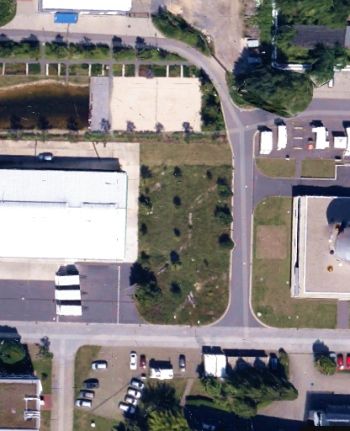
M. Schrön et al.: Intercomparison of cosmic-ray neutron sensors in an urban environment                                         87

equivalent θ uses the following relation:                           (counts per a hours), where a is an arbitrary factor following
                                                                    τa = a τ . In order to keep cph as the standard reference unit
                    0.0808                                          for all neutron time series, the units can be transformed back
θ(N ) · %bulk =                − 0.115 − θoffset ,           (2)
                  N/N0 − 0.372                                      to τ (i.e. 1 h). Then the average count rate and uncertainty
                                                                    become
where %bulk (in g cm−3 ) is the soil bulk density, θoffset (in
g/g) is the gravimetric water equivalent of additional hydro-                 1 Xa
                                                                          Na =   1
                                                                                   N ≈ hN i ,
gen pools (e.g. lattice water, soil organic carbon), and N0                   a
                                                                                                                               (5)
(in counts per hour, cph) is a free calibration parameter (for                1                 1
                                                                                qX
                                                                                   a
                                                                    σ (Na ) =        σ (N )2 ≈ √ hσ (N )i .
details see Desilets et al., 2010; Bogena et al., 2013). The                  a    1             a
latter can be calibrated using the count rate N and inde-
pendent measurements of the average water content hθ i in             As a consequence, the average statistical error of a daily
the footprint. According to Schrön et al. (2017a) the CRNS          aggregated time series (in units of cph) is given as σ (hNi) =
probe does not measure a simple, equally weighted average           √
                                                                      hNi /24, which corresponds to 80 % less uncertainty com-
of the surrounding water content due to the non-linearity of        pared to hourly resolution.
its radial sensitivity function, Wr (h, θ ). Therefore, different
parts of the footprint area contribute differently to the av-       2.4.3    Performance measures
erage signal depending on their distance r from the sensor.
This knowledge can be used to quantify the contribution of          The spread of individual sensors around their average hNi
individual areas that are of specific interest.                     can be expressed as
                                                                                 "                 #1/x
2.4.2    Counting statistics                                                  1X
                                                                    σx (N ) =     |Ni − hNi|x             ,                    (6)
                                                                              9 i
Nine CRNS probes were employed for the intercomparison
study and each member of the CRNS ensemble acts as an
                                                                    where the parameter x determines the distance norm. Then,
individual monitoring system. The co-location of these sen-
                                                                    σx=1 is defined as average absolute deviation, and σx=2 ≡ σ
sors, however, offers a unique opportunity to combine their
                                                                    is the standard deviation.
signals, which leads to high total count rates and thus lower
                                                                       The Pearson correlation coefficient can be defined for two
statistical noise. The average count rate hNi and its propa-
                                                                    time series NA and NB with standard deviations σA and σB :
gated uncertainty σ of each ith sensor are given as
                                                                                     (NA − hNA i) · (NB − hNB i)
           1X                                                       ρ(NA , NB ) =                                .             (7)
    hNi =         Ni ,                                                                       σA · σB
           9
                                                             (3)
           1 X
             q
σ (hNi) =                  2
                    σ (Ni ) ,
           9                                                           For example, ρ = 0.7 depicts that NA and NB can explain
                √                                                   0.72 ≈ 50 % of their respective variance. If those two vari-
where σ (N ) = N is given as the standard deviation of av-          ables, NA and NB , were ranked depending on the order of
erage counts N using Gaussian statistics, and 9 is the number       their magnitude, Ni 7 −→ rank(Ni ), the Pearson correlation
of individual sensors used in this study. Under the assump-         turns to the so-called Spearman rank correlation:
tion that Ni ≈ Nj ∀i, j ∈ (1, . . ., 9), their corresponding un-                                                      2
                                                                                            P
certainty will be similar as well:                                                           t rank(N A ) − rank(N B )
                                                                    ρS (NA , NB ) = 1 − 6                                  ,   (8)
         σ (Ni ) ≈ hσ (Ni )i ∀i ,                                                                    n(n2 − 1)
                   1
                     q
                                                                    where n is the total number of intervals and t ∈ (1, . . ., n).
⇒       σ (hNi) ≈      9 · hσ (Ni )i2                        (4)
                   9                                                This quantity can be used to identify events that changed the
                   1               1p                               rank of specific sensors.
                 = hσ (Ni )i ≈        hNi .
                   3               3
                                                                    2.5     The neutron transport simulator URANOS
Hence, the combination of nine sensors reduces the relative
statistical error by ≈ 67 %, thereby allowing for accurate          The generation, interaction, and detection of neutrons can
measurements of changes of the environmental water stor-            be simulated with Monte Carlo codes, which are based on
age.                                                                physically modelled interaction processes, and state-of-the-
   Temporal aggregation can further reduce the standard de-         art nuclear cross section databases. The Ultra Rapid Adapt-
viation. The measurement interval τ is usually set to 1 h,          able Neutron-Only Simulation (URANOS) has been specif-
while the count rate N is given in units of cph. Aggregation        ically tailored to environmental neutrons relevant for CRNS
of the time series N to longer intervals leads to the series Na     research. The model was described by Köhli et al. (2015)

www.geosci-instrum-method-data-syst.net/7/83/2018/                          Geosci. Instrum. Method. Data Syst., 7, 83–99, 2018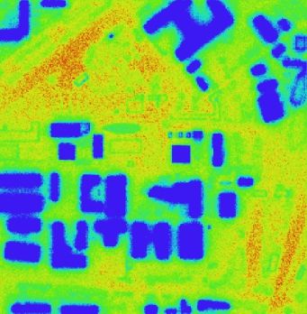
88 M. Schrön et al.: Intercomparison of cosmic-ray neutron sensors in an urban environment
Table 1. Two soil profiles in the grass meadow sampled nearby the WSN is a promising tool in the field of environmental sci-
profiles of the wireless sensor network (WSN) on 14 January 2016. ence to detect and record energy and matter fluxes across
Samples were taken with core cutters of constant volume at three Earth’s compartments (Hart and Martinwz, 2006; Zerger
depths, oven-dried, and weighted according to standard procedures. et al., 2010; Corke et al., 2010). The WSN used in this study
The evaporated water content is given in units of volumetric percent. was developed specifically for short-term, demand-driven ap-
plications (Mollenhauer et al., 2015; Bumberger et al., 2015).
Profile Depth %bulk in g cm−3 Porosity 2 Water θ
The soil moisture sensors of type Truebner SMT100 used
in the soil profiles directly measure electrical permittivity, ε,
South 7–12 cm 1.62 38 % 18 % which is a compound quantity of the individual media (water,
South 15–20 cm 1.52 42 % 15 %
soil, air) and their volumetric fractions in the soil (Brovelli
South 25–30 cm 1.58 40 % 18 %
North 5–10 cm 1.60 40 % 32 %
and Cassiani, 2008). The volumetric water content θ was de-
North 15–20 cm 1.93 27 % 19 % duced from ε with the CRIM formula (Roth et al., 1990),
North 25–30 cm 1.91 28 % 28 % using independent measurements of porosity and soil wa-
ter temperature and assuming randomly aligned microscopic
soil structures. The measurement uncertainties in units of
to calculate the footprint volume and spatial sensitivity of absolute volumetric percent could be related to the device
CRNS probes. It has since been successfully applied to ad- (< 2 %) and could vary from wet to dry conditions. They
vance the method of cosmic-ray neutron sensing (Schrön are highly dependent on prior calibration (Truebner, 2012)
et al., 2015, 2017a) and also to advance research in nuclear and may be related to inappropriate assumptions on the per-
physics to simulate neutron detectors and characterize their mittivity of quartz (< 3 %) and to the heterogeneity of soil
response on the millimetre scale (Köhli et al., 2016, 2018). properties and composition in the meadow (< 8 %). The lat-
One of the unique features is the simulation of spatial neu- ter uncertainty was tested by sampling soil moisture profiles
tron densities in an arbitrary, user-defined terrain. URANOS at many places within the field and is taken into account when
is very flexible and allows to input spatial bitmap information WSN is compared to CRNS observations.
about the materials and geometries in the studied area. The
software comes with a graphical user interface and is freely 2.7 Measurement Strategy
available (see www.ufz.de/uranos).
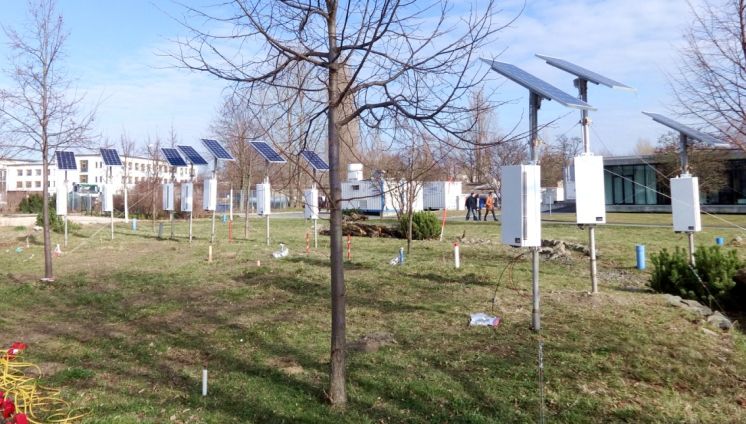
The urban scenario of 500 m × 500 m around the CRNS
probes was re-enacted using 2-D images of different lay- The study site is an urban area at the Helmholtz Centre
ers that represent the different material compositions. More for Environmental Research – UFZ in Leipzig, Germany
than 145 million neutrons were released equally distributed (51◦ 210 1100 N, 12◦ 260 0200 E; 116 m above sea level). The site
in heights of 80 to 50 m. The simulation domain in total cov- exhibits humid climatic conditions and consists mainly of
ered a volume of 900 m × 900 m and 1000 m height, where grassland patches surrounded by sealed areas such as roads
the additional padding around the area accounts for border and buildings (Fig. 2).
effects. Non-sealed area was defined as grassland with an In February 2014, nine cosmic-ray neutron sensors were
exemplary soil moisture of 30 %. Buildings were modelled installed in a small grass meadow to monitor the neutron den-
as blocks of air by a 0.5 m concrete wall. Trees were mod- sity in air. The sensors were co-located within a maximum
elled as blocks of organic material with 0.3 kg m−3 biomass distance of 15 m, which was assumed to be small relative to
stretching to heights of up to 20 m. Details of all materials the sensor footprint. The individual count rates were logged
used can be found in the Supplement of this paper. Simu- every 15 min and were processed using the standard correc-
lated neutrons were counted in a detector layer 1.75 m above tion approaches described above.
the surface, representing the typical position of cosmic-ray Dedicated experiments were prepared (Table 2) to test the
neutron sensors. hypotheses whether a potential sensor-to-sensor variability is
influenced by the location of the sensors (hypothesis A), by
2.6 Point-scale soil moisture measurements device-specific differences (hypothesis B), or by statistical
noise (hypothesis C). In Phase I, the sensors were operated
In order to validate and calibrate the sensors against inde- in the initial arrangement (see Fig. 2) for 3 weeks. Before
pendent soil water content, two measurement methods were entering Phase II, four sensors were swapped, while five sen-
consulted to quantify soil moisture profiles: volume soil sam- sors kept their position to serve as a reference. A comparison
ples (single measurement) and a mobile wireless ad hoc soil between Phase I and Phase II allows us to observe the effect
moisture network (WSN) (continuous). The measurements of potential locational effects on the sensor response. After 4
were taken in different depths at two locations near the CRNS weeks, detection parameters were adjusted to reduce the ob-
probes. The corresponding soil parameters (Table 1) and time served device-specific differences and to test their influence
series data have been utilized to calibrate the neutron signal on the count rates when entering Phase III. In all phases, the
on volumetric soil moisture using Eq. (2). correlation between the sensors and its dependence on tem-
Geosci. Instrum. Method. Data Syst., 7, 83–99, 2018 www.geosci-instrum-method-data-syst.net/7/83/2018/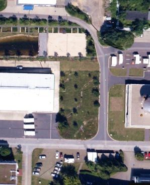
M. Schrön et al.: Intercomparison of cosmic-ray neutron sensors in an urban environment                                                      89

Table 2. Measurement strategy to investigate the sensor-to-sensor variability (Phase I), the influence of location (Phase II), the effects of
detector parameters (Phase III), the heterogeneity of neutrons within the sensor’s footprint (Survey), and the sensor’s capabilities to monitor
soil moisture in the complex, urban terrain.

              Experiment       Period                             Description
              Phase I          2014-02-22 to 2014-03-18           initial arrangement of the nine sensors
              Phase II         2014-04-07 to 2014-05-08           permuted positions of sensors 1, 2, 3, 4, 8
              Phase III        from 2014-05-09                    adjusted detector parameters of all sensors
              Survey           2014-05-02, 2015-07-22             spatial mapping of neutron heterogeneity with a CRNS rover
              Validation       2015-09-29 to 2015-10-31           comparison with soil moisture from a wireless ad hoc sensor network

                                                                                   Finally, the performance of the CRNS soil moisture prod-
                                                                                uct in such a complex terrain was questioned. The WSN was
                                                                                installed in two soil profiles near the CRNS sensor arrange-
                                                                  Tree
                                         Pond          Sand                     ment in order to evaluate the capabilities of the neutron sen-
                                                                                sor to estimate water content in the urban environment.
                                                           CRNS

                                         Building

                                                                                3     Results and discussions
                                                                   Grass
                                                Concrete                        3.1    The influence of sensor location

                                                                                The nine co-located sensors were operated in their initial ar-
 5000 m                                 10 m                                    rangement for 3 weeks (Phase I). While all sensors showed
                                                                                similar trends, prominent offsets were observed between in-
                                                                                dividual signals, particularly for sensors 3 and 4 (Fig. 3). The
                                                                                average deviation of all count rates from their ensemble
                                                                                                                                    √      mean
                                                                                exceeded the daily statistical error, σ (N24 h ) ≈ 600/24 =
                                                                                5, by a factor of 2.
                                                                                   Although the maximum distance between the sensors was
          2     3 4 5      6   7
                                                                                only 15 m, it has been hypothesized that the individual loca-
                                                                         9      tions could have introduced a systematic effect on the count
                                                              1
                                                                                rate due to the steep radial sensitivity curve (Köhli et al.,
                                                       8
                                                                                2015; Schrön et al., 2017a). This hypothesis A has been
                                                                                tested by observing the change of neutron count rates be-
                                                                                fore and after the change of their position within the sensor
Figure 2. Location and arrangement of the nine cosmic-ray neu-                  arrangement.
tron sensors deployed at the small, urban meadow at UFZ Leipzig,                   Before the second phase positions of a subset of sensors
Germany.                                                                        were swapped, while others remained fixed (Fig. 4a). In order
                                                                                to assess the effect on their individual measurement offsets,
                                                                                Spearman rank correlations were applied to the time series
poral aggregation was investigated to test the influence of re-                 before and after sensor permutation (see Fig. 4b). This quan-
duced statistical uncertainty.                                                  tity explains the probability with which a sensor’s count rate
   In order to fully understand implications of hypothesis A,                   N is assigned to an ordered rank among the ensemble. The
i.e. the effects of location on the sensor response, we per-                    data showed that the favoured rank (or offset) of both fixed
formed URANOS simulations of the site-specific neutron                          and swapped sensors was almost unaffected. In particular, the
distribution and conducted spatial surveys in parts of the                      ranks of sensors 3 and 4 remained at their high or low levels,
CRNS footprint area. The spatial distribution of neutrons                       respectively.
was measured with the mobile CRNS rover detector in a car                          Figure 3 further suggests that small-scale positioning has
(May 2014) and on a hand wagon (July 2015). To achieve a                        not been the main cause of the individual variability, as only
spatial resolution in the range of a few metres, the rover was                  subtle changes of the deviation of the sensor signals from
operated at walking speed.                                                      their mean were found between phases I and II. Neverthe-
                                                                                less, the subtle changes can be quantified in more detail by
                                                                                looking at the counting efficiencies of the sensors (i.e. rela-

www.geosci-instrum-method-data-syst.net/7/83/2018/                                     Geosci. Instrum. Method. Data Syst., 7, 83–99, 2018
90                              M. Schrön et al.: Intercomparison of cosmic-ray neutron sensors in an urban environment

                 Phase I.               Phase II.                 Phase III.                                              Rain in mm
                                                                                                                                   0
     Neutrons
      N in cph
                                                                                                                                   10
                                                                                                                                   20
                                                                                                                                   30
                                                                                                                                   40
                                                                                                                                   50

       700

                                                                                          Sensors                    Mean
                                                                                              #1        #4           #7
       650                                                                                    #2        #5           #8
                                                                                              #3        #6           #9

       600

                                                                                               SD from mean
         10                                                                                    Stat. counting error
          9
          8
          7
          6
          5
          4
              21 28   7 14       11 18 25     2               16 23 30     6   13 20 27                  4     11    18     25
             Feb Feb Mar Mar     Apr Apr Apr May              May May May Jun Jun Jun Jun               Jul    Jul   Jul    Jul

Figure 3. Time series of nine sensors covering phases I (installation), II (permutation), and III (calibration) in year 2014. By removing
detector-specific effects in Phase III, the standard deviation (SD) of the sensor ensemble from their mean could be reduced down to the
statistical error of σ ≈ 5 cph.

tive deviation from their mean) in Fig. 5. The efficiency can          3.2     Detector-specific variability
be estimated either theoretically, by the relative positions of
the lower discriminator in the PHS, or empirically, by the
variability of the observed neutron counts. Figure 5 shows             Phase III was dedicated to the diagnosis of the count rate,
the theoretical relative efficiency of the nine sensors before         which is directly related to the integral of the PHS. As ex-
Phase III and their empirical values in phases I, II, and III.         plained in Sect. 2.3.2, the shape of the PHS and the param-
   The results indicate that different components are con-             eters used to determine its integral (such as the lower dis-
tributing to the total sensor-to-sensor variability. The theo-         criminator) are important for the individual sensor efficiency.
retical, detection-specific efficiency from the PHS processor          Thus, consistent detection parameters are a prerequisite to
accounts for only 0.77 % mean deviation, which cannot ex-              assure that the same fraction of neutron capture events are
plain the high empirical values of 1.87 and 1.64 % in phases           counted by all detectors. The inconsistent spectra in Fig. 6
I and II, respectively. Furthermore, the fact that swapped sen-        (dotted black line) indicate that this requirement was not met
sors changed their mean efficiency by −0.37 %, while fixed             before Phase III. Are these device-specific differences having
sensors only changed by −0.04 % from Phase I to Phase II               an influence on the intercomparability of the neutron signals
indicates that one of the additional variability components            (hypothesis B)?
might be related to location.                                             To achieve comparability of the pulse height spectra
   All in all, a small positional effect cannot be excluded            among the sensors, we set the lower discriminator consis-
(confirming hypothesis A), but the major part of the observed          tently below the wall effect shelf (around bin 24) and ad-
sensor-to-sensor variability must have originated from other           justed the high voltage and amplifier gain parameters such
sources.                                                               that the main peaks aligned approximately to bin number 100
                                                                       for the sake of visual accessibility. This procedure ensured
                                                                       maximum count rate for the individual sensors.
                                                                          In Fig. 6 (left) the resulting change of the PHS is shown
                                                                       for all sensors, and the impact on the neutron count rate is

Geosci. Instrum. Method. Data Syst., 7, 83–99, 2018                          www.geosci-instrum-method-data-syst.net/7/83/2018/
M. Schrön et al.: Intercomparison of cosmic-ray neutron sensors in an urban environment 91
lower amplitude neutron pulse events that were previously
Phase I. II. Sensor permutation being filtered by the lower discriminator.
(a) Phase I. Phase II. In terms of relative variation (Fig. 5), the adjustment of the
detector parameters at the beginning of Phase III caused the
sensor efficiencies to change from 1.64 to 0.52 %. Thereby
2
3 the detector-specific variability was almost removed and the
4 1 sensors have since shown the best agreement to each other.
5 6 5 6 The remaining variability could be contributed to small
7 7 differences in design and geometry from the manufacturer
8 or the sensor location. The overall variability of 0.52 % is
4
3 now comparable with the standard relative error of the daily
9 mean, σ (N )/N, which went down to 0.55 % in certain peri-
8 1 9 2
ods of this study.
3.3 Temporal resolution for consistent observations
1m The previous sections have shown that the CRNS probes ex-
(b) Rank correlation hibited small but measurable sensor-to-sensor variability that
Phase I. Phase II.
1 was related to positional effects and to the factory configura-
No. 1 No. 2 No. 3 tion of the neutron detector operating parameters. This sec-
tion tests hypothesis C, the potential influence of statistical
0.5 noise to the sensor intercomparability. The statistical vari-
ability component is related to the random nature of neutron
0 detection. According to Sect. 2.4.2, the corresponding uncer-
1 tainty can be reduced by temporal aggregation. This is ex-
No. 4 No. 5 No. 6
( xed) ( xed) pected to influence the correlation between the nine CRNS
0.5 probes. While Bogena et al. (2013) calculated the uncertain-
ties for several temporal resolutions theoretically, the present
arrangement provides a unique opportunity for an experi-
0
mental approach with multiple sensors.
1 Figure 7a shows that the ensemble-averaged correlation of
No. 7 No. 8 No. 9
( xed) ( xed) the nine sensors significantly increased with increasing in-
0.5 tegration time across the three phases. The correlation coef-
ficient was 0.12 and 0.26 for 1 h integration time and went
0 up to 0.61 and 0.74 for 10 h in phases I and II, respectively.
1 2 3 4 5 6 7 8 1 2 3 4 5 6 7 8 1 2 3 4 5 Rank Since the sensor swap itself should have no effect on the cor-
relation, the difference between Phase I and Phase II could
Figure 4. (a) Birds-eye view on the sensor arrangement before and
be attributed solely to the meteorological dynamics in these
after permutation of sensors 2, 3, 4, and 8. (b) Rank correlations of
the nine CRNS signals before (dotted) and after (solid) permutation. periods. While rain events were almost absent during Phase I
Both swapped and fixed sensors showed no significant change. (compare Fig. 3), the corresponding neutron dynamics were
mainly influenced by statistical and detector-specific vari-
ability. In Phase II, a number of rain events led to large am-
plitudes of neutron count dynamics and thus naturally to in-
demonstrated exemplarily for sensor 3. The parameter ad- creased correlations.
justments shifted the main PHS peak towards bin 100, and The highest correlation was achieved in Phase III,
the reduction of the lower discriminator effectively increased when most of the detector-specific variability was removed
the neutron count rate of the sensor. After manual adjust- (Sect. 3.2). Moreover, correlation coefficients exceeded a
ment of the parameters for all sensors, most of the individual value of 0.90 for more than 6 h of integration time and went
offsets vanished and the standard deviation from the mean, up to 0.97 for daily aggregation. These results demonstrate
σ (N ), was reduced by 50 % down to the order of the sta- the reliability of CRNS observations for integration times
tistical error (compare Fig. 3). Moreover, the average ab- of at least 6 h under humid conditions, in complex terrain,
solute deviation
√ was reduced even below the statistical er- and at sea level. Even higher correlations can be expected for
ror σ (N ) = N/24 of the daily aggregated time series (not dry regions and homogeneous terrain at high altitude, where
shown). All in all, the instruments showed greater consis- higher neutron count rates and less structural disturbances
tency in neutron counting sensitivity since the recovery of would lead to lower noise.
www.geosci-instrum-method-data-syst.net/7/83/2018/ Geosci. Instrum. Method. Data Syst., 7, 83–99, 201892 M. Schrön et al.: Intercomparison of cosmic-ray neutron sensors in an urban environment
+3
(deviation from the mean)
Mean squared
Relative efficiency in %
+2 deviation in %
+1 PHS 0.77
Phase I 1.87
0
Phase II 1.64
-1 Phase III 0.52
-2
Change I II
-3 Swapped -0.37
Fixed -0.04
Sensor no. 1 2 3 4 5 6 7 8 9
( xed) ( xed) ( xed) ( xed)
Figure 5. Relative deviation of the neutron count rates around their ensemble mean, calculated before (Phase I) and after (Phase II) the
swap of sensor positions and after adjusting the detector parameters (Phase III). In addition, theoretical values before Phase III have been
determined from the location of the discriminator in the pulse height spectrum (PHS, black). Error bars are based on the standard deviation
of the count rate for each sensor.
experiments using spherical neutron detectors (Figs. 8–9 in
Phase II. III. Detector parameter calibration Rühm et al., 2009).
Pulse height spectra Neutrons in cph
No. 1 3.4 Spatial heterogeneity in the footprint area
760
No. 2
Parameter change for sensor no. 3
The previous sections have confirmed that there is a mea-
No. 3 surable positional effect (hypothesis A), that device-specific
740
No. 4 variability exists (hypothesis B), and that statistical noise
contributes to the measurement uncertainty (hypothesis C).
No. 5
720
Solutions have been found to overcome the latter two is-
No. 6 sues by adjusting the detector parameters or by aggregating
No. 7 the temporal resolution, respectively. But what can be done
700
to better understand the influence of local structures in the
No. 8
CRNS footprint?
No. 9
680
Positional effects within a few metres can occur and
40 60 Bin 100 1 May 2 May 3 May
should be taken into account, although their effect was shown
to be less important than the detector-specific variability.
Figure 6. Adjustment of the detector parameters harmonized the Several of the conducted observations supported the hypo-
pulse height spectra of the nine sensors (before: dotted black) and thetical influence of local effects within the complex terrain.
increased their range towards the lower left end. The impact on the For example, Fig. 3 shows high variability of neutron count
count rate is shown exemplarily for sensor 3 (orange). rates in drying periods and low variability in wetting peri-
ods. This could be an effect of the dynamic size of the foot-
print and of the varying rates of evaporation and dewfall.
According to Köhli et al. (2015), the distance which neu-
The accuracy of the CRNS soil moisture product also im- trons travelled before detection is smaller for wetter condi-
proves for higher integration times. In Fig. 7b the effect of tions. Thereby, distant structures could lose influence during
the temporal aggregation of neutron counts is propagated to and after rain events and thus would contribute to a harmo-
the individual soil moisture products θ (Ni ), where their root- nization of the nine sensor count rates. A second observation
mean-square errors (RMSEs) against the ensemble mean refers to Fig. 5, where noticeable changes of variability were
θ(hNii ) are plotted. For all sensors, RMSEs were reduced by observed for swapped sensors (phase transition I→II), while
50–70 % using daily aggregation, while an accuracy of 1 % the behaviour of fixed sensors was almost unchanged.
gravimetric water content was achieved beyond integration The two examples indicate that local effects might have
times of 6 h. These findings agree quantitatively with theo- the potential to influence the sensor performance. Local sen-
retical calculations by Bogena et al. (2013) and with similar sitivity of the neutron detectors has been augured already by
Geosci. Instrum. Method. Data Syst., 7, 83–99, 2018 www.geosci-instrum-method-data-syst.net/7/83/2018/M. Schrön et al.: Intercomparison of cosmic-ray neutron sensors in an urban environment 93
(a) Pearson correlation (b) RMSE (in grav. %) of sensor soil moisture against their mean
Phase I. Phase II. Phase III.
1.0 5
No. 1
No. 2
0.8 4 No. 3
No. 4
0.6 3 No. 5
No. 6
No. 7
0.4 Phase I 2 No. 8
Phase II No. 9
Phase III
0.2 1
Ensemble
spread
0.0 0
0 5 10 15 20 0 5 10 15 20 0 5 10 15 20 0 5 10 15 20
Integration time in h Integration time in h
Figure 7. Influence of integration time, in hours (h), on the correlation and performance among the ensemble of nine sensors. (a) Ensemble-
average Pearson correlation of the nine signals by twos for phases I, II, and III and temporal aggregation from 1 to 24 h. (b) Root mean square
error of the individual soil moisture products against the soil moisture product of the ensemble mean hNi. Accuracy below gravimetric water
contents of 1 % can be achieved for all sensors when sensor-specific offsets were removed (Phase III) and the integration time exceeds 6 h.
Köhli et al. (2015) and could be a reasonable explanation ficient to support the theory of highly heterogeneous patterns
given the heterogeneous distribution of the soil, of vegeta- in the urban terrain.
tion, and of nearby structures. This section tries to further Both experimental and theoretical results clearly demon-
quantify the local effects in a moisture-averaging footprint strate that a significant neutron heterogeneity can occur
of several tens of hectares, where all sensors are exposed to within the CRNS footprint under conditions of complex ter-
similar meteorological forcings. rain. These patterns have the potential to influence the CRNS
To assess the influence of complex terrain in the urban measurements. Moreover, slight variability is evident in the
area, neutron transport simulations were conducted with the small meadow (centre cross in Fig. 8), where trees and struc-
Monte Carlo code URANOS (Sect. 2.5). The model calcu- tures might influence the neutron density on a scale of a
lated the neutron response to the structures in the footprint few metres. This could serve as an explanation for the mi-
and simulated the neutron density that could be potentially nor position-related variability observed in the course of this
observed with CRNS detectors in the whole area. Figure 8c study.
shows features of low and high neutron counts on the metre
scale that are related to the effects of buildings, sealed areas, 3.5 Soil moisture estimation and areal correction for
the pond, iron-containing structures, and vegetation. Under sealed areas
these conditions it is evident that local heterogeneity in the
footprint can have an effect on CRNS probes located within Considering the revealed small-scale heterogeneity in the
a distance of a few metres. sensor footprint, as well as large sealed areas around the sen-
The URANOS model can help to assess those effects to sors, the important question arises whether CRNS in urban
support optimal sensor positioning or to explain unusual fea- areas will be able to reliably estimate environmental water
tures in the spatial signal. The simulation results demonstrate content. Therefore, we have evaluated the CRNS soil mois-
the non-uniformity of the neutron density in the footprint. ture product (Eq. 2) with time series data from two nearby
However, the simulated quantities are not expected to exactly profiles using the WSN. The locations (crosses) of each pro-
match reality due to many modelling assumptions that have file are shown in Fig. 9; the data were averaged and compared
been put into the scenario (clean material composition, uni- against the CRNS signal of sensor 7 (point).
form biomass density, homogeneous soil moisture). Never- Figure 9 shows that the CRNS soil moisture product (or-
theless, the modelled patterns can be assessed visually us- ange) differs significantly from the point measurements (grey
ing measurements from a CRNS rover (Fig. 8d, e). The rela- dashed). Most importantly, the response to rain events ap-
tive uncertainties of both the modelled and measured results pears to be much more damped in the CRNS signal. A damp-
are in the range of 6–9 % for ≈ 200 modelled neutrons per ing effect can occur when a constant fraction of measured
m2 and ≈ 200 measured neutrons per minute. A direct com- neutrons is independent of precipitation events.
parison with the simulation results was not intended, as the The CRNS probe’s footprint is much larger than the small
low number of measurement points does not allow for metre- meadow of 0.1 ha where the CRNS and the WSN probes are
scale predictions of neutron density from the ordinary krig- located. It is thus evident that the paved and sealed areas be-
ing interpolation. However, the collected data have been suf- yond the meadow could bias the integral soil moisture signal.
www.geosci-instrum-method-data-syst.net/7/83/2018/ Geosci. Instrum. Method. Data Syst., 7, 83–99, 201894 M. Schrön et al.: Intercomparison of cosmic-ray neutron sensors in an urban environment
a
200 m
(a) Birds-eye view (Google Maps)
(b) Abstract map of materials
for input to URANOS
building concrete road grass
100
iron tar road roof grass
vegetation water pool gas pipe
wood sand tartan ground
(c) Relative neutron density, simulated
0
with URANOS
0.6 0.7 0.8 0.9 1.0
-100
(d) Relative neutron density, measured
with Rover, Kriging interpol. of points
(e) (d) May 2, 2014. (e) Jul 22, 2015
-200
0.6 0.7 0.8 0.9 1.0
-200 -100 0 100 200 m
b c
P S P S
d e
P S P S
Figure 8. (a) Neutron environment of the urban CRNS test site (centred black cross). (b) Abstract model of the area using geometric shapes
and colour-coded material definitions. (c) URANOS simulation of epithermal neutrons in a detector layer above the surface. (d, e) Measured
neutrons with the mobile CRNS rover confirm heterogeneity of neutron patterns in the centred grass meadow as well as in the surrounding
urban domain.
Geosci. Instrum. Method. Data Syst., 7, 83–99, 2018 www.geosci-instrum-method-data-syst.net/7/83/2018/M. Schrön et al.: Intercomparison of cosmic-ray neutron sensors in an urban environment 95
A circular section of angle ϕ (in radiant), which is confined
between radii r1 and r2 , contributes the following fraction of
Tree neutrons n:
Pond Sand
1 ϕ r2
Z Z
n(r1 , r2 , ϕ) = Wr (h, θ ) · dr · dϕ 0
2π 0 r1
Building (10)
ϕ r2
Z
CRNS = Wr (h, θ ) · dr .
2π r1
Grass WSN
Concrete
The contribution area of the grassland meadow and sur-
Grass area
equivalent rounding patches is roughly equivalent to a circle of radius
10 m
circle r2 ≈ 20 m. Hence, the portion of measured neutrons from this
Water area is n(0, r2 ) ≈ 41 ± 2 %, depending on h and θ. The dry
equiv. Rain and sealed areas beyond the grass meadow are effectively
in % Intercepted damping the otherwise highly dynamic signal from the soil
water (orange line in Fig. 9).
25
CRNS To remove this damping effect, we suggest a new method
20
corrected to rescale the dynamic component of the neutron signal that
is influenced by both a variable and a constant patch in the
15 CRNS footprint. At the urban test site, only 0.1 ha of the footprint
Soil contains soil, beyond which everything else is either paved
10 probe area or solid building. Thus, only a small fraction n(r1 , r2 , ϕ)
of the total neutrons is connected to soil moisture variability.
Sep 29 Oct 06 Oct 13 Oct 20 Oct 27 In order to compare these measurements with independent
Figure 9. Top: illustration of the circular area (dashed) around the
soil moisture sensors, we introduce an areal correction,
CRNS probe 7 that confines an area equivalent to the non-sealed N − hNi
grassland meadow. Bottom: demonstrating the area correction ap- Ncorr = + hNi , (11)
n(r1 , r2 , ϕ)
proach (Eq. 11). The constant contribution of neutrons from the
sealed area leads to a damped signal of soil moisture dynamics mea- that essentially scales the anomaly of neutrons by the inverse
sured by the CRNS (orange line). The corrected signal (blue line) fraction of the contributing area, where h·i denotes the tem-
shows more pronounced dynamics based only on the areal contri-
poral mean. Using the corrected data from the CRNS probe
bution of the meadow. The remaining deviation (shaded blue) from
(blue line) and the average soil moisture from the two profiles
the WSN soil moisture measurements (grey dashed) probably rep-
resents intercepted water over the sealed ground during and after (grey), Fig. 9 demonstrates that this scaling approach brings
rain events. both signals into good agreement and is therefore helpful to
interpret CRNS data with confined areal coverage.
Besides the improved match of soil moisture dynamics, the
area-corrected signal apparently overestimates soil moisture
We suspect the dry soil under the sealed surface in the foot- peaks during and after rain events. This can be interpreted as
print of having a constant and thus damping influence on the a representation of an important hydrological feature in urban
neutron signal. In the following, we aim to test the applica- areas. When the whole footprint is considered for data inter-
tion of recent insights about the sensor’s spatial sensitivity pretation, it becomes evident that the CRNS should be sen-
and demonstrate how this knowledge can help to understand sitive to precipitation water ponded on buildings and paved
and even correct the biasing effect of sealed areas. ground before it eventually evaporates. Therefore, the addi-
Following theoretical considerations from Köhli et al. tional water seen by the CRNS probe following rain events
(2015) and robust evidence from Schrön et al. (2017a), the can be suspected of representing the intercepted water over
radial sensitivity function Wr (h, θ ) depicts the number of de- sealed areas.
tected neutrons that originated from the distance r under cer-
tain homogeneous conditions of air humidity, h, and (soil)
water equivalent, θ . Its integral across all distances represents 4 Summary and conclusion
the total number of neutrons detected, N:
This intercomparison study was motivated by the observa-
tion of unknown variability in CRNS data and by the aim
Z∞ to understand how reliable and reproducible soil moisture
N = Wr (h, θ ) · dr . (9) data could be generated using the method of cosmic-ray neu-
0
tron sensing. To address the open questions, we co-located
www.geosci-instrum-method-data-syst.net/7/83/2018/ Geosci. Instrum. Method. Data Syst., 7, 83–99, 201896 M. Schrön et al.: Intercomparison of cosmic-ray neutron sensors in an urban environment
nine CRNS measurement stations within a 5 m ×15 m grass- approach the influence of sealed (and thus constantly dry) ar-
land area, surrounded by complex urban terrain. Three main eas in the footprint can be quantified and the corresponding
hypotheses were investigated and the following conclusions damping effects removed. The quantification of the sensitiv-
were drawn: ity to local patches in the footprint is particularly meaning-
ful for supporting hyper-resolution land surface modelling
A. We claimed that the sensor location has an influence on (e.g. Chaney et al., 2016) and precision agriculture. The latter
the neutron measurement. The hypothesis was tested by includes targeted irrigation based on information about soil
swapping the position of four out of nine CRNS probes. properties, plant variety, and density (Hedley et al., 2013; Pan
We found the influence on the neutron counts is mea- et al., 2013). In addition to soil moisture, the CRNS probe ap-
surable, but insignificant within a few metres. However, peared to be sensitive to intercepted water over sealed areas.
mobile surveys as well as neutron simulations indicated Such information could be used to actually quantify intercep-
that neutron abundance can be highly heterogeneous tion and evaporation processes (see e.g. Baroni and Oswald,
within the sensor’s footprint, making the signal prone 2015) and could eventually contribute to closing the water
to local effects on scales above a few metres. balance.
In future studies we would recommend to further assess
B. Device-specific differences were suspected of being re-
the potential of cosmic-ray neutron sensors for urban hydrol-
sponsible for systematic variations in the CRNS signal.
ogy. Since water in complex terrain is almost impossible to
This was tested with the help of the manufacturers by
quantify with point sensors, the large-scale averaging capa-
consistently adjusting neutron detection parameters and
bilities of cosmic-ray neutron probes could be a promising
aligning the pulse height spectra of the nine sensors. The
advantage for urban sciences.
detection parameters were found to have significant in-
fluence on the count rate by up to 3 %. The adjustment
led to a reduction of the total contribution of systematic
Data availability. The multi-sensor dataset is available in the Sup-
errors down to the order of the statistical counting er- plement of this paper.
rors. We recommend applying this adjustment in order
to achieve consistent measurements among sensors.
C. Statistical noise was suspected to be the reason for much The Supplement related to this article is available online
of the remaining variability that hinders comparability at https://doi.org/10.5194/gi-7-83-2018-supplement.
of neutron signals. We applied temporal aggregation to
the neutron signals and looked at the correlation and en-
semble spread of the CRNS products. Sensors showed
correlations below 0.6 for hourly data and above 0.9
Competing interests. Darin Desilets and Gary Womack are affili-
for aggregation of 6 h and beyond. In the same manner
ated with Hydroinnova LLC, the manufacturer of the probes used
the RMSE between the soil moisture products improved in this study.
from 2 % down to 0.9 % gravimetric percent. If multiple
standard CRNS detectors are required to deliver similar
results under similar conditions, a minimum temporal Acknowledgements. We thank Uwe Kappelmeyer (UFZ) for
resolution of 6 h was found to provide acceptable com- providing meteorological data from a nearby UFZ-owned weather
parability for humid climate at sea level. This value can station. We acknowledge the NMDB database www.nmdb.eu,
be considered as an upper limit, as it gets further re- founded under the European Union’s FP7 programme (contract
duced by drier climates, higher altitudes, and more sen- no. 213007) for providing data for incoming radiation, especially
sitive detectors. from monitors Jungfraujoch (Physikalisches Institut, University of
Bern) and Kiel (Institute for Experimental and Applied Physics,
This work highlights the importance of studies on sensor- University of Kiel). Martin Schrön acknowledges kind support by
to-sensor intercomparison for geoscientific instruments. the Helmholtz Impulse and Networking Fund through Helmholtz
Those efforts can reveal unexpected features or systematic Interdisciplinary School for Environmental Research (HIGRADE).
errors, can highly improve the understanding of the sensor Mandy Kasner was funded by the Helmholtz Alliance EDA –
response, and will thus improve their application in environ- Remote Sensing and Earth System Dynamics, through the Initiative
and Networking Fund of the Helmholtz Association, Germany. The
mental sciences. One of the impacts of this study has already
research was funded and supported by Terrestrial Environmental
led to improved efforts to adjust the detection parameters
Observatories (TERENO), which is a joint collaboration program
during the manufacturing process. involving several Helmholtz Research Centres in Germany.
The CRNS water equivalent measured in the urban en-
vironment has shown remarkable agreement with indepen- The article processing charges for this open-access
dently measured soil moisture profiles when accounted for publication were covered by a Research
the sealed-area effect. With the proposed “areal correction” Centre of the Helmholtz Association.
Geosci. Instrum. Method. Data Syst., 7, 83–99, 2018 www.geosci-instrum-method-data-syst.net/7/83/2018/You can also read