Incarceration, Earnings, and Race - WP 21-11 Grey Gordon Federal Reserve Bank of Richmond - Federal Reserve Bank of ...
←
→
Page content transcription
If your browser does not render page correctly, please read the page content below

Incarceration, Earnings, and Race

   WP 21-11           Grey Gordon
                      Federal Reserve Bank of Richmond

                      John Bailey Jones
                      Federal Reserve Bank of Richmond

                      Urvi Neelakantan
                      Federal Reserve Bank of Richmond

                      Kartik Athreya
                      Federal Reserve Bank of Richmond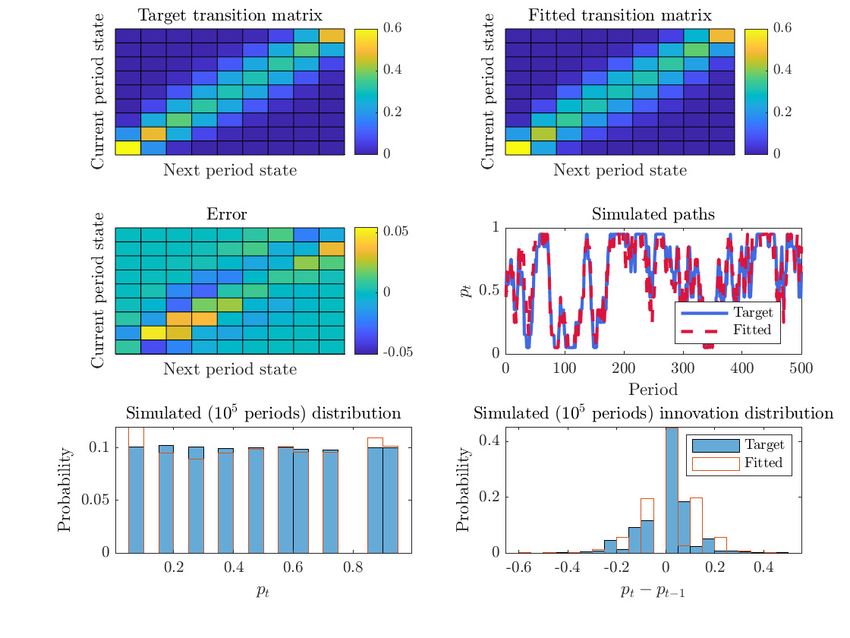
Incarceration, Earnings, and Race∗
        Grey Gordon†             John Bailey Jones‡               Urvi Neelakantan§
                                      Kartik Athreya¶

                                        July 2, 2021

                                           Abstract
          We study the implications of incarceration for the earnings and employment
       of different groups, characterized by their race, gender, and education. Our
       hidden Markov model distinguishes between first-time and repeat incarceration,
       along with other persistent and transitory nonemployment and earnings risks,
       and accounts for nonresponse bias. We estimate the model using the National
       Longitudinal Survey of Youth 1979 (NLSY79), one of the few panel datasets
       that includes incarcerated individuals. The consequences of incarceration are
       enormous: First-time incarceration reduces expected lifetime earnings by 39%
       (59%) and employment by 8 (13) years for black (white) men with a high
       school degree. Conversely, nonemployment and adverse earnings shocks increase
       expected years in jail. Among less-educated men, differences in incarceration
       and nonemployment can explain a significant portion of the black-white gap in
       lifetime earnings—44% of the gap for high school graduates and 52% of the gap
       for high school dropouts.

       Keywords: earnings dynamics, incarceration, racial inequality
       JEL Codes: C23, D31, J15
   ∗
      We are grateful to Amanda Michaud for helpful comments and to Thomas Lubik and Mark
Watson for early guidance. Emily Emick and Luna Shen provided excellent research assistance. The
views expressed here are those of the authors and should not be interpreted as reflecting the views
of the Federal Reserve Bank of Richmond or the Federal Reserve System.
    †
      Federal Reserve Bank of Richmond
    ‡
      Federal Reserve Bank of Richmond
    §
      Federal Reserve Bank of Richmond
   ¶
      Federal Reserve Bank of Richmond

                                                1
1 Introduction
Between 1980 and 2016, the incarceration rate in the United States rose from 0.22% to
0.67% (US Department of Justice, Bureau of Justice Statistics, 2018). The impact of
this three-fold increase has fallen disproportionately on those who are male, black, or
less educated: The imprisoned population is overwhelmingly (91-93%) male and less
educated (Ewert and Wildhagen, 2011), and the imprisonment rate for black men
(2.2%) is nearly six times that for white men (US Department of Justice, Bureau
of Justice Statistics, 2019, Table 10).1 Within certain groups, incarceration is now
pervasive: Western and Pettit (2010, Table 1) find that among black high school
dropouts born between 1975 and 1979, 68% had been incarcerated at least once.
Despite the prevalence and growth of incarceration in the United States, much
remains unknown about the relationship between incarceration, employment, earn-
ings, and demographics.2 Our goals in this paper are to (1) quantify the dynamic
relationship between incarceration, employment, and earnings and (2) measure the
contribution of incarceration and other forms of nonemployment to the earnings gap
between black and white men.3 To this end, we estimate a statistical model of in-
carceration, employment, and earnings over the life cycle, using a flexible framework
that controls semi-parametrically for race, education, and gender. Our hidden Markov
model allows for transitory and persistent nonemployment spells, movements up and
down the (positive) earnings distribution, and arbitrarily long-lasting effects of incar-
ceration. Transition probabilities depend on age, gender, race, education, and previ-
ous incarceration. We estimate the model using the National Longitudinal Survey of
Youth 1979 (NLSY79), one of the few panel datasets that reports incarceration. We
explicitly account for missing data and allow for the possibility that its incidence is
not random.
1
The majority of style guides currently recommend that neither “black” nor “white” be capital-
ized, so we follow this convention. The incarceration rate and the imprisonment rate are distinct
measures, as only the former includes people held in local jails. While the measure we use in our
analyses is incarceration, many national statistics are available only for the imprisoned.
2
As Neal and Rick (2014) observe, there is a need for more research on the effects of incarcera-
tion on “the employment and earnings prospects of less-skilled men, and less-skilled black men in
particular.”
3
Although we study both men and women, we focus on reporting results for men because they
comprise the vast majority of the incarcerated. We report a few results and statistics for women in
Section 5 and in the Appendix. Additional results are available upon request.
2Our estimates show that the income losses associated with incarceration and long-
term nonemployment are enormous. A typical 25-year-old black (white) male high
school graduate entering jail for the first time will, relative to an otherwise identical
man, suffer a lifetime income loss of $121,000 ($273,000) in 1982-1984 dollars, a 40%
(54%) drop. For those without a high school degree, the losses amount to $103,000
and $170,000, respectively, resulting in 54% and 49% drops (respectively) for black
and white men. The large lifetime effects are a consequence of essentially permanent
reductions in flow earnings after an incarceration spell. The earnings losses from a
transition to persistent nonemployment are also significant. For black male high school
graduates, the loss ($113,000) is comparable to the loss from incarceration, while the
loss for white men ($154,000) is somewhat smaller.
Although the effects of incarceration and nonemployment are profound for both
black and white men, their incidence differs markedly. For high school graduates, our
estimates indicate that while 24% of black men will eventually be incarcerated, only
3% of white men will.4 Differences in nonemployment outside of incarceration are
also quite large. Between ages 22 and 57, black men with a high school degree will on
average experience 8.5 years of nonemployment, 4.5 years more than whites.
To summarize, the likelihood of nonemployment and incarceration is higher for
black men than for their white counterparts, while the effects on earnings are typi-
cally larger for white men. What, then, is the net effect of these forces on the lifetime
earnings gap between the two groups?5 One way we answer this question is to elim-
inate incarceration and/or nonemployment and recalculate the gap. In the baseline,
white male high school graduates earn 65% more than black male high school grad-
uates over their lifetimes. Eliminating incarceration alone would reduce this to 59%,
while eliminating nonemployment alone would reduce it to 44%. If both incarceration
and nonemployment were eliminated, the lifetime earnings of white male high school
graduates would exceed those of black males by 37%. Alternatively, a formal decom-
position suggests that 46% of the lifetime earnings gap for high school graduates is
attributable to nonemployment and/or incarceration. This fraction is higher (67%)
4
Because the NLSY79 cohort came of age before the height of the incarceration boom, their
incarceration rates, while high, fall below those realized at the height of the boom.
5
We again use numbers for male high school graduates, but again, similar patterns hold across
all education levels.
3for high school dropouts and lower (20%) for college graduates.
In addition to our substantive findings, our paper introduces a rich yet relatively
tractable framework for earnings processes. Our framework integrates nonemploy-
ment, incarceration and earnings, imposes few distributional assumptions, and builds
on a well-established statistical literature. Whenever incarceration, or more gener-
ally any discrete outcome, is important to understanding earnings, our framework
provides a flexible way to account for it.
1.1 Related literature
Our paper contributes to three bodies of work: the study of the impact of incarceration
on employment and earnings, the study of the black-white earnings gap, and the study
of earnings processes in general.
The data show unambiguously that “labor market prospects after prison are bleak”
(Travis et al., 2014, page 233). In their review (and borrowing from Pager, 2008),
Travis et al. (2014) discuss three potential explanations. The first is selection: Indi-
viduals with poor job market prospects are more likely to acquire a criminal record.6
The second is transformation: Time spent in jail or prison changes individuals in ways
undesirable to employers. The third is labeling: A history of imprisonment in and of
itself makes an individual less desirable to employers. There are legal restrictions
(and/or liability concerns) regarding what positions those with a criminal record can
fill. Moreover, consistent with the first two mechanisms, a criminal record may signal
undesirable traits.
The leading empirical issue in this literature is controlling for the first mecha-
nism, non-random selection into incarceration. Travis et al. (2014) describe several
methodological responses. Among studies using survey data, the leading strategy is
to construct “control groups” of nonincarcerated individuals who otherwise resemble
the incarcerated. This has many parallels with our approach, where we condition on
an individual’s incarceration and earnings history, as well as their education, gender,
and race. These studies generally find that incarceration depresses subsequent labor
market outcomes. Among studies using administrative data, a popular strategy is to
6
Throughout the document, we use “criminal record” to mean a record that includes time spent
in jail or prison.
4exploit exogenous variation in incarceration due to the random assignment of judges
(Kling 2006, Loeffler 2013, Mueller-Smith 2015). As a whole, studies that use admin-
istrative data—with or without the judge instrument—provide mixed support for a
causal interpretation.7
Like most models of earnings processes, our framework is statistical, and episodes
of incarceration therein are not strictly exogenous. On the other hand, most individ-
uals in our data go to jail or prison after we first observe them, allowing us to show
that individuals with low earnings are more likely to transition into incarceration.
Moreover, the NLSY79 cohort happened to live through a period where aggregate
incarceration rates increased dramatically, implying that much of the variation in
incarceration is exogenous to the individual.
Irrespective of whether incarceration is driven by worker characteristics or by
chance, it is valuable to know how labor market outcomes change in its aftermath,
and our framework allows us to do this. In particular, our framework allows us to track
earnings and employment for decades, enabling us to study the long-run dynamics
and cumulative effects of incarceration.
In addition to the purely empirical literature discussed by Travis et al. (2014),
there are a number of structural studies that incorporate incarceration, including
Lochner (2004), Fella and Gallipoli (2014), Fu and Wolpin (2018), and Guler and
Michaud (2018). These generate earnings losses in various ways. For example, Guler
and Michaud (2018) assume that incarceration leads to human capital depreciation
and a higher proclivity for crime. Relative to these structural studies, our approach
allows for a more flexible specification, with a rich set of age and demographic controls.
Our results can also complement structural analyses by providing estimation targets
like those used in Guler and Michaud (2018).
Our paper also contributes to the empirical literature on the black-white earnings
gap. As Bayer and Charles (2018) document, this gap has proven remarkably per-
sistent: As a proportion of the median earnings of white men, the median earnings
of black men are no higher today than they were in 1950. They attribute much of
the difference to a large and expanding gap in employment; the gap in median earn-
7
This may reflect limitations of administrative data; although accurate, most administrative
sources have fewer variables, explanatory or outcome, than do surveys.
5ings among male workers has in fact narrowed considerably.8 As the growth of the
employment gap has coincided with the surge in incarceration, it is natural to ask
whether the two are related.
The third literature to which our paper contributes is the estimation and anal-
ysis of earnings processes. This literature is huge; an incomplete list of papers in-
cludes Abowd and Card (1989), Meghir and Pistaferri (2004), Bonhomme and Robin
(2009), Guvenen (2009), Bonhomme and Robin (2010), Altonji et al. (2013), Hu
et al. (2019), De Nardi et al. (2020) and Guvenen et al. (2020). Our paper adds to
this literature in three ways. The first is that it explicitly accounts for incarceration.
Earlier earnings process studies have not differentiated between incarceration and
other forms of nonemployment. Because of data limitations—many data sets exclude
the institutionalized—they might not have had the capacity to do so. Second, many
earnings process studies have focused on the continuously employed. Our approach
combines incarceration, nonemployment, and positive earnings in a unified frame-
work. This allows us to account for the possibility that incarceration is likely to be
preceded, as well as followed, by low earnings.9
We also make a methodological contribution to the literature. Like Arellano et al.
(2017), we define transition probabilities in terms of quantiles, rather than levels,
which allows for nonnormal shocks and variable persistence. We target a different
set of quantiles, however, which allows us to utilize existing work on latent Markov
Chains (e.g., Bartolucci et al. 2010, Bartolucci et al. 2012). One advantage of our
framework is that it allows us to differentiate between short- and long-term spells of
nonemployment. Hence, we can capture varying levels of labor market attachment.
Our framework also lets us deal with missing data flexibly, allowing its incidence to
be nonrandom and persistent over time.
The rest of the paper is organized as follows. In section 2, we introduce our sta-
tistical model, and in section 3, we describe the data. In section 4, we interpret our
parameter estimates. In section 5, we discuss the model’s implications for employment,
8
Bayer and Charles (2018) also emphasize the role of race-neutral increases in the returns to
education, which have amplified the effects of education differences.
9
In estimating the earnings process for their structural model, Caucutt et al. (2018) assume that
ex-convicts transition into either unemployment or the lowest possible positive earnings quintile. On
the other hand, they assume that the probability that an individual becomes incarcerated in the
future depends only on whether the individual is incarcerated at present.
6incarceration, and earnings over the life-cycle and calculate the changes in lifetime
earnings and employment that follow an episode of incarceration. In section 6, we
assess the contributions of incarceration and other forms of nonemployment to the
racial gap in lifetime earnings. We conclude in section 7.
2 Statistical Model and Methodology
Our model of earnings contains two variables: an unobserved latent state that follows
a Markov chain; and a discrete-valued observed outcome, the distribution of which
depends only on the current latent state. This is a variant of the ubiquitous state-space
framework, arguably most akin to Hamilton’s (1989) regime-switching model.10
2.1 Latent States and Observed Outcomes
Let `n,t ∈ L = {L0 , L1 , ..., LI−1 } denote individual n’s underlying, latent labor mar-
ket state at date t, and let mn,t ∈ M = {M0 , M1 , ..., MJ−1 } denote the earnings
outcome observed by the researcher. The set of latent states, L, consists of incarcer-
ation, long-term nonemployment, and Q∗ earnings potential bins.11 This set of latent
outcomes is then interacted with a {0, 1} criminal record flag, so that L contains
I = 2(Q∗ + 2) elements. The set of observed outcomes, M, consists of incarceration,
current nonemployment, Q positive earnings bins, and not interviewed/missing. The
nonmissing outcomes are also interacted with the criminal record flag, so that M
contains J = 2(Q + 2) + 1 elements.
We discretize the distributions of both earnings potential and observed earnings
(when positive). This both simplifies the estimation process and produces estimates
that port directly into dynamic structural models. As we show below, we can increase
the number of earnings bins without increasing the number of model parameters. It
also bears noting that the bins represent quantile rank (conditional on race, gen-
der, education, and age), rather than level, groupings. As the extensive literature on
copulas (see, e.g., Trivedi and Zimmer 2007) has shown, working in quantile space
10
See also Farmer (2020). Bartolucci et al. (2010) provide an introduction.
11
An individual’s earnings potential is his or her unobserved earnings capacity.
7is an effective way to model non-normal shocks and variable persistence.12 Let pq ,
where q = 0, 1, ..., Q, denote the probability cutoffs for the earnings bins; in a modest
abuse of notation we will also use q to index the bin given by the interval (pq−1 , pq ),
q = 1, 2, ..., Q. We partition earnings into deciles, so that pq ∈ {0.0, 0.1, ..., 0.9, 1}, and
there are Q = 10 bins. We assume further that the bins for latent earnings potential
are the same as those for observed earnings, so that Q∗ = Q; this is straightforward if
tedious to relax. We estimate the deciles for observed earnings, semi-parametrically,
in a separate procedure.
Our model is based on two key assumptions. The first is that `n,t is conditionally
Markov, with the I × I transition matrix, Ax :
Aj,k | x = Pr(`n,t+1 = Lk | `n,t = Lj , xn,t ) = Pr(`n,t+1 = Lk | Ft ), (1)
where: xn,t is a vector of exogenous variables; Ft denotes the time-t information set;
and Aj,k | x denotes row j and column k of Ax . In our case, xn,t contains an individual’s
age (which enters parametrically) and their race, gender, and education level (which
enter semi-parametrically, as there are separate sets of parameters for each group).13
The second assumption is that the distribution of the observed outcome mn,t depends
on only the contemporaneous realization of `n,t . We place the probabilities that map
`n,t to mn,t in the I × J matrix Bz :
Bj,k | z = Pr(mn,t = Mk | `n,t = Lj , zn,t ) = Pr(mn,t = Mk | Ft−1 , `n,t ). (2)
The vector zn,t is the concatenation of xn,t and an indicator of whether the individual
was interviewed in period t − 1, which captures the persistence of nonresponse. The
final element of our model is the 1 × I row vector µ1 , which gives the unconditional
distribution of the initial latent state `n,1 conditional on xn,1 .
For the remainder of the section, we will drop the individual index n and suppress
the probabilities’ dependence on x and z.
12
Arellano et al. (2017) also rely heavily on quantiles, for similar reasons. As we discuss in Ap-
pendix A, however, the structure of their approach is very different from ours.
13
Recall that `n,t includes whether the individual has been previously incarcerated.
8Figure 1: Earnings process transitions
Current Latent State: lt
{ Jail, Not Employed, bin1, bin2, …, binQ* }
Logit Transition Probabilities
Transition
bins 1 through Q*
Matrix A: lt → lt+1
Kumaraswamy CDF: depends on lt
Jail Not Employed bin1 bin2 … binQ*
Observation Matrix B: lt+1 → mt+1
Not
Jail Not Employed bin1 bin2 … binQ
Interviewed
2.2 Latent State Transitions
As the top half of Figure 1 shows, we populate the transition matrix A in two steps.
First, we use a multinomial logit regression to determine the one-period-ahead prob-
abilities of incarceration, long-term nonemployment, or employment (bins 1 to Q∗ ).
We assume that an incarceration record is backward-looking and permanent, so that
once a person is incarcerated, he will have an incarceration record in all subsequent
periods.
The variables in this regression include the current state, age, and interactions.
Appendix A presents our exact specification. An important simplification is that we
characterize the earnings potential bins by their midpoint rank, p̃q := [pq +pq−1 ]/2. By
way of example, when earnings are partitioned into deciles, p̃q ∈ {0.05, 0.15, ..., 0.95}.
Because we treat p̃q as continuous rather than categorical, the number of variables in
the logistic regression is invariant to the number of bins.
Second, we estimate the distribution of next period’s earnings potential, condi-
tional on being employed, across the bins. To do this, we assume that the conditional
distribution of ranks follows the Kumaraswamy (1980) distribution. Like the Beta
9distribution, the Kumaraswamy distribution is a flexible function defined over the
[0, 1] interval; however, its CDF is much simpler:
K(p; α, β) = Pr(y ≤ p; α, β) = 1 − (1 − pα )β .
The parameters α and β are both strictly positive. It follows that if earnings bin q
covers quantiles pq−1 to pq ,
Pr(bin q) = K(pq ; α, β) − K(pq−1 ; α, β). (3)
We allow α and β to depend on the current state `t and the explanatory vector xt , so
that α = α(`t , xt ) and β = β(`t , xt ). When the current state is the earnings bin qt , we
characterize it by its midpoint value, p̃qt . Appendix A presents the full specification.
Our functional forms place relatively few restrictions on the earnings transi-
tions. As Jones (2009) argues, the Kumaraswamy distribution appears well-suited
for “quantile-based” statistical modeling, permitting a wide variety of shapes. More-
over, given enough terms, α(·) and β(·) can vary in arbitrarily complicated ways,
allowing the conditional CDF K p; α(`t , xt ), β(`t , xt ) to vary in arbitrarily compli-
cated ways. Strictly speaking, our approach is valid only when the true conditional
distribution of earnings potential is smooth. This is a standard assumption, however,
and we have separate nonemployment and incarceration states that absorb the mass
of zero-earnings outcomes. In Appendix B, we assess the ability of the Kumaraswamy
distribution to approximate a standard Gaussian AR(1) process and show that the
approximation works well.
Because we use the midpoint value p̃qt to characterize the current earnings bin,
the number of parameters in α(·) and β(·) need not increase with the number of bins
(see Appendix A). Even if we treat α(·) and β(·) as sieve estimators, the number of
parameters will grow more slowly than the sample size. As the number of bins grows
large, we get the conditional CDF K pt+1 ; α(pt , xt ), β(pt , xt ) , where pt and pt+1 are
both quantile ranks; at this point, K(·) is a copula. The probability difference in equa-
tion (3), appropriately deflated, likewise converges to the density of the underlying
Kumaraswamy distribution.
102.3 Observation Dynamics
The bottom half of Figure 1 shows how we populate the observation matrix B. The
first step of the process is determining the probability that an individual is interviewed
by the NLSY at time t.14 We use a logistic specification. The explanatory variables
include the current latent state, age, and an indicator of whether the individual was
interviewed in the previous wave. Including these variables helps us control for non-
random attrition.
Conditional on being observed, we impose the following mapping from latent states
to measured outcomes. We assume that the NLSY79 measures incarceration accu-
rately, so that the latent incarceration state maps directly into the incarceration
outcome. Because our latent nonemployment state is meant to capture long-term
disengagement from the labor force, we assume the persistent nonemployment state
maps directly into nonemployment (again, conditional on being observed). Finally,
each earnings potential bin can map into nonemployment and any of the observed
earnings bins. The probability of nonemployment is logistic. Conditional on being
employed, the distribution of earnings across bins follows a formula akin to equa-
tion (3), the main difference being that the Kumaraswamy distribution is replaced by
a truncated univariate logistic distribution. Because multiple combinations of A and
B can produce similar patterns of observed outcomes, we seek a specification where
the distribution of observed earnings shifts rightward in earnings potential. Using the
symmetric logistic distribution, which we further center around the earnings potential
rank p̃q , ensures that the mapping from the latent states to the observed outcomes
has this property.
In the standard earnings model, transitory shocks capture both short-term earn-
ings shocks and measurement error. A similar sort of ambiguity applies here. We
believe that transitions from latent earnings to nonemployment reflect short-term
spells of nonemployment. Transitions between latent and observed employment bins
may reflect measurement error as well.
14
Individuals who die are dropped from the likelihood function at their date of death, rather
than treated as missing. We view attrition via death as qualitatively distinct from nonresponse. For
similar reasons, we also remove individuals when they are dropped from the NLSY79’s Supplemental
Sample in 1991.
112.4 Initial Probabilities
We construct the initial distribution of latent states, µ1 (`1 |x̃1 ), in much the same
way we found their transition probabilities. (Here, x̃1 consists of race, gender, and
education.) First, we find the probability that the individual is incarcerated, nonem-
ployed (long-term), or in one of the earnings potential bins. Conditional on having
positive earnings, we find the distribution across initial earnings potential bins using
the Kumaraswamy distribution; the calculations parallel those in equation (3). The
final step is to estimate the probability that the individual has a criminal record, con-
ditional on the other latent states, using a logistic regression. The product of these
two probabilities gives us our initial distribution.
2.5 Likelihood
We estimate our model using maximum likelihood, utilizing the forward recursion
described in, e.g., Bartolucci et al. (2010) and Scott (2002). This is quite similar to
the methodology for the regime-switching model presented in Hamilton (1994, chapter
22). Appendix A provides a more detailed description. We estimate separate sets of
transition and observation probabilities for each race-gender-education combination.
We weight each individual’s log-likelihood using the NLSY79 sampling weights for
1979.15
For some groups—white men with a college degree, white women with at least a
high school diploma, and black women with either a high school or a college degree—
the incidence of incarceration is so low that their incarceration-related parameters
cannot be estimated with any precision. In these cases, we drop individuals with
a criminal record and estimate a simplified model of employment and earnings. To
this set of parameters, we add incarceration-related parameters estimated for other,
similar groups, namely white men with some college education, white women without
a high school diploma, or black women with some college experience. In making
these imputations, we adjust the constant terms for the incarceration probabilities
to match the ever-incarcerated rate observed for that group in the NLSY79;16 with a
15
Within each race-gender-education group, the weights are scaled to have an average value of 1.
16
For white men and black women with college degrees, and white women with a high school
degree, the fraction of individuals with a criminal record is implausibly low, 0.03% or less. In these
12logistic formulation, this is simple to do. Appendix F describes the adjustments. These
imputations are somewhat ad hoc, but the groups to which they are applied have
very low rates of incarceration, implying that any imputation error will be relatively
unimportant in the aggregate.
2.6 Quantiles and Conditional Means
To complete our model, we need to delineate the earnings bins and assign a level of
earnings to each bin. We estimate bin cutoffs by age, for each race-gender-education
group, using quantile regression. Using these cutoffs, we then assign individuals to
bins and take averages by age. While the estimation procedure works with any set
of cutoffs, to reduce sampling error we estimate the cutoffs and within-bin condi-
tional means from the Current Population Survey (CPS), which contains far more
observations than the NLSY79.
3 Data
We now describe how we use our two data sources, the NLSY79 and the CPS.
3.1 The NLSY79
Our primary source of data is the 1979 cohort of the National Longitudinal Survey of
Youth (NLSY79), a nationally representative panel survey of young men and women
born between 1957 and 1964. From 1979-1994, respondents were interviewed every
year; since 1994, interviews occur every other year. The NLSY collects information
about education, employment, family, and finances. It is also one of the few nationally
representative surveys that enables us to observe an individual’s incarceration status.
Specifically, the variable that reports a person’s residence status and location allows
“jail/prison” as a response.17 Coupled with the available earnings and employment
data, this information makes the NLSY79 well-suited for our study and enables us to
carry out our analysis largely using this single dataset.
cases we impute the rates using data from other race and education groups.
17
We use “jail” henceforth to refer to either jail or prison.
13The NLSY79 has three subsamples: the (core) cross-sectional sample, a supple-
mental sample of minority and/or disadvantaged individuals, and a military sample.
We exclude the military sample, as earnings for this group are hard to interpret, and
we drop Hispanic respondents. This leaves us with roughly 9,600 individuals, of which
4,747 are male. We include both workers and the self-employed; Appendix C describes
our employment and earnings measures in some detail.
We have four education categories: less than a high school diploma, high school
diploma, some college, and bachelor’s degree or higher. Exploiting the panel design of
the NLSY79, we classify individuals on the basis of their highest observed attainment,
treating education as a permanent characteristic. We categorize individuals by years
of schooling, except for GED recipients, whom we classify as high school dropouts. As
Heckman et al. (2011) and others have noted, GED recipients on average have worse
labor market outcomes than those receiving high school diplomas. It is also the case
that many recipients earn their GEDs while incarcerated.
Table 1 shows summary statistics for men, the main focus of our analysis.18 Our
data cover the years 1980-2014. The first panel illustrates the education gradient in
earnings and shows that at every education level, black men earn significantly less than
their white counterparts. By way of example, median earnings for a black high school
dropout are 41% (4.93/12.00) those of his white counterpart. The second panel shows
incarceration rates. For most groups, incarceration rates are highest for men in their
30s. This may reflect to some extent a conflation of time and age effects: The national
transition toward mass incarceration in the 1980s and 1990s occurred at the same time
the NLSY79 cohort aged out of their 20s and into their 30s. Another notable feature
is that men with some college experience are more likely to be incarcerated than high
school graduates; recall that we classify GED recipients as high school dropouts. As
expected, incarceration rates differ markedly by race. The largest absolute differences
are among high school dropouts: The difference across all ages is over 6 percentage
points (pp). The largest proportional differences, however, are among those with at
least a high school degree.
The third panel of Table 1 shows our measure of a “criminal record,” namely a
personal history of at least one previous incarceration spell.19 The fourth panel shows
18
Appendix D shows the summary statistics for women. Statistics calculated using 1979 weights.
19
Because our measure of a criminal record is backward-looking, our estimation sample starts in
14Table 1: Summary Statistics by Race and Education for Men, NLSY79
Black Men White Men
LTHS HS SC CG LTHS HS SC CG
Earnings (in $1,000s)
Mean 7.73 11.90 14.35 24.00 13.45 19.65 22.53 32.44
10th percentile 0 0 0 0.93 0 4.29 2.91 3.01
25th percentile 0 2.74 4.99 10.11 4.40 11.01 10.90 12.32
50th percentile 4.93 10.50 13.20 19.21 12.00 17.57 18.69 24.11
75th percentile 12.32 17.06 20.48 30.60 18.55 25.08 28.07 38.42
90th percentile 19.35 24.90 28.80 45.93 26.57 34.21 40.38 65.22
Currently Incarcerated (%)
All ages 9.61 2.54 3.40 0.41 3.30 0.26 0.53 0.01
22-29 10.87 2.10 3.13 0.69 3.60 0.25 0.59 0
30-39 12.39 4.03 4.59 0.24 3.23 0.41 0.58 0
40-49 5.93 1.84 2.74 0 3.26 0.09 0.55 0
50 and older 3.02 0.67 1.69 0.66 1.98 0.07 0 0.11
Previously Incarcerated (%)
All ages 27.52 9.75 9.21 2.80 13.18 0.95 2.44 0.02
22-29 18.72 4.40 5.89 1.99 9.23 0.45 1.38 0
30-39 31.11 10.95 10.13 3.01 13.29 0.99 2.82 0
40-49 34.55 14.65 13.17 3.85 19.11 1.50 3.32 0
50 and older 35.87 16.94 11.36 3.14 19.74 1.87 3.89 0.21
Fraction Employed (%)
All 55.00 69.90 71.21 78.51 68.56 78.25 77.48 81.44
Previously 32.17 41.60 33.62 47.89 46.09 43.66 53.31 50.00
incarcerated
Not previously 63.55 72.98 75.03 79.45 71.91 78.56 78.04 81.43
incarcerated
Mean Values
Year of birth 1960.4 1960.4 1960.4 1960.3 1960.5 1960.2 1960.1 1960.3
Age 29.76 30.05 28.80 29.77 27.62 27.86 28.09 28.99
Fraction of male 4.67 4.76 3.01 2.12 15.61 28.12 17.37 24.34
population (%)
Observations 8,475 9,071 5,829 3,935 10,035 16,081 9,755 14,315
Individuals 479 499 322 209 781 1,016 603 838
Note: [LTHS,HS,SC,CG] denote less than high school/high school/some college/college
graduate.
15employment. The first row of this panel, which shows aggregate results, reveal that
the earnings gaps found in the first panel are to some extent employment gaps. This
is consistent with the findings of Bayer and Charles (2018) described earlier: The
earnings gaps among the fully-employed, although still significant, are smaller. The
second and third rows of this panel show that the employment rates for men with
a criminal record are 25-40pp lower than those of men without. There may also be
incarceration-related differences in the earnings of those who work.
The final panel shows the distribution of respondents by race and education. The
first line shows proportions calculated using the NLSY79 sample weights, while the
last two lines show unweighted counts. Including the supplemental sample provides
us with a large number of black respondents.
3.2 The Current Population Survey (CPS)
Although the NLSY79 is our principal data source, to calculate the cutoffs that de-
lineate the earnings quantiles, we make use of the larger sample available in the CPS
(downloaded from IPUMS; Ruggles et al. 2020). CPS data are available from 1962 to
2019; however, we limit our sample to 1976 onward because data on hours worked,
which we need for our measure of employment, are not available prior to that year.
Since the CPS is not a panel, we employ a synthetic cohort approach. Ideally, we
would limit the sample to those born in the same years as our NLSY79 cohort (1957
to 1964) but, to have a sufficient number of observations, we include individuals born
between 1941 and 1980 (i.e., the NLSY79 +/- two cohorts) and use cohort dummies
to account for any cohort effects within this group. This consists of around 4.2 mil-
lion observations. We restrict the sample to white and black individuals, who together
make up about 94% of the sample. We also exclude those for whom educational at-
tainment is not reported. We limit observations to those aged between 22 and 66.
Starting the sample at age 22 helps ensure that those who chose to attend college
have entered the workforce. We choose 66 as the upper limit since that is the nor-
mal Social Security retirement age for the NLSY79 cohort. After applying these age
restrictions, around 3 million individuals remain in the sample.
The CPS elicits income information for the year prior to the survey year. Our
1980, allowing us to use the 1979 incarceration measure.
16focus is on earnings, which we define broadly to include not just wage and salary in-
come, but also the labor portions of farm and business income. Since we have separate
categories for the nonemployed and incarcerated, we limit ourselves to those who were
employed in the previous year. Those who remain (about 2.4 million) form our sample
of employed individuals. Appendix C describes our employment and earnings mea-
sures in more detail. We weight the data to ensure that the sample is representative
of the population.
Within this sample, we estimate earnings bin cutoffs (deciles) separately for each
race-gender-education group. In particular, in each group, for each quantile q, we run
the following quantile regression:
5
X
yt = βq,0 + βq,1 at + βq,2 a2t + βq,3 a3t + γq,m cohortm + q,t . (4)
m=2
Here yt denotes earnings, at is age, and cohortm is a dummy variable for one of the
five 8-year cohorts contained in our CPS sample.
With the results of Equation (4) in hand, we use post-estimation procedures to
obtain the decile cutpoints for each race-gender-education-cohort group at each age.
These are shown in Figures E.1 and E.2 for women and men, respectively, in Ap-
pendix E.
Applying the cutpoints to the CPS data, we calculate within-decile mean earnings
at each age for each group. We then fit a cubic polynomial in age with cohort dummies
through these age-specific means. Applying post-estimation procedures to the results
of this regression yields life-cycle profiles of within-decile mean earnings for our cohort
of interest. Figures E.3–E.4 show mean earnings and the fitted life-cycle profiles for
women and men from the 1957-64 birth cohort.
4 Estimation Results
Given the nonlinear nature of the underlying model, the parameter estimates and
standard errors, displayed in Tables F.1 and F.2 of Appendix F, are hard to interpret.
Consequently, we instead highlight a few of the implied transition matrices (A) and
observation matrices (B).
174.1 Latent Transition Matrices
We focus our discussion of the transition matrices on men without a high school
degree, where the dynamics of incarceration are easiest to see, but all education
groups display similar patterns. Tables 2 and 3 present the latent state transition
probabilities for a 25-year-old black man and white man, respectively, without a high
school degree. Rows index the current state `t , while columns index the future state
`t+1 .20
Table 2: Latent transition probabilities, 25-year-old black men without a high school
diploma
Future State
Jail Flag = 0 Jail Flag = 1
Current Q1+ Q3+ Q5+ Q7+ Q9+ Q1+ Q3+ Q5+ Q7+ Q9+
State ↓ N Q2 Q4 Q6 Q8 Q10 Jail N Q2 Q4 Q6 Q8 Q10 Jail
JF = 0 N 0.73 0.17 0.03 0.02 0.01 0.01 0.02
JF = 0 Q1 0.14 0.52 0.18 0.06 0.01 0.00 0.08
JF = 0 Q3 0.05 0.27 0.53 0.11 0.00 0.00 0.04
JF = 0 Q5 0.02 0.01 0.23 0.63 0.09 0.00 0.02
JF = 0 Q6 0.01 0.00 0.07 0.53 0.37 0.00 0.01
JF = 0 Q8 0.01 0.00 0.01 0.12 0.55 0.31 0.01
JF = 0 Q10 0.00 0.00 0.00 0.02 0.08 0.89 0.00
JF = 0 Jail 0.16 0.31 0.10 0.06 0.03 0.01 0.34
JF = 1 N 0.56 0.18 0.03 0.02 0.01 0.01 0.18
JF = 1 Q1 0.07 0.35 0.13 0.05 0.01 0.00 0.39
JF = 1 Q3 0.03 0.20 0.44 0.10 0.00 0.00 0.23
JF = 1 Q5 0.01 0.01 0.19 0.58 0.09 0.00 0.12
JF = 1 Q6 0.01 0.00 0.06 0.48 0.37 0.00 0.09
JF = 1 Q8 0.00 0.00 0.01 0.11 0.52 0.31 0.05
JF = 1 Q10 0.00 0.00 0.00 0.02 0.08 0.87 0.03
JF = 1 Jail 0.04 0.10 0.04 0.02 0.01 0.00 0.79
Note: Rows are indexed by the latent state at age 25, columns by the latent state at age 26. JF or
Jail Flag indicates a history of incarceration. “Jail” denotes currently incarcerated. N indicates not
employed but not currently incarcerated. Qi denotes earnings potential decile i. Some transitions
omitted.
The first of these general patterns is that men who are nonemployed or have low
earnings potential are much more likely to transit to jail. A 25-year-old black man
20
To avoid presenting 242 numbers, we condense the matrix A in two ways: We present transition
probabilities for only a subset of the current states, reducing the number of rows; and we combine
future states by summing probabilities, reducing the number of columns.
18with no criminal history (JF = 0) in the bottom decile of the earnings potential
distribution (Q1) has a roughly 8% chance of becoming incarcerated at age 26. The
incarceration probability for an otherwise identical man in the 8th earnings potential
decile (Q8) is 1%. White men follow the same pattern, though their corresponding
chances of being incarcerated are lower than for black men.
Table 3: Latent transition probabilities, 25-year-old white men without a high school
diploma
Future State
Jail Flag = 0 Jail Flag = 1
Current Q1+ Q3+ Q5+ Q7+ Q9+ Q1+ Q3+ Q5+ Q7+ Q9+
State ↓ N Q2 Q4 Q6 Q8 Q10 Jail N Q2 Q4 Q6 Q8 Q10 Jail
JF = 0 N 0.69 0.17 0.06 0.04 0.02 0.01 0.01
JF = 0 Q1 0.05 0.71 0.18 0.02 0.00 0.00 0.04
JF = 0 Q3 0.03 0.28 0.63 0.04 0.00 0.00 0.02
JF = 0 Q5 0.02 0.00 0.17 0.76 0.05 0.00 0.01
JF = 0 Q6 0.01 0.00 0.02 0.52 0.44 0.00 0.00
JF = 0 Q8 0.01 0.00 0.00 0.03 0.64 0.31 0.00
JF = 0 Q10 0.00 0.00 0.00 0.00 0.06 0.93 0.00
JF = 0 Jail 0.04 0.45 0.12 0.04 0.01 0.00 0.34
JF = 1 N 0.71 0.11 0.05 0.03 0.03 0.03 0.05
JF = 1 Q1 0.05 0.52 0.18 0.05 0.01 0.00 0.18
JF = 1 Q3 0.03 0.25 0.56 0.07 0.00 0.00 0.08
JF = 1 Q5 0.02 0.00 0.17 0.70 0.07 0.00 0.04
JF = 1 Q6 0.01 0.00 0.03 0.48 0.46 0.00 0.02
JF = 1 Q8 0.01 0.00 0.00 0.04 0.56 0.38 0.01
JF = 1 Q10 0.00 0.00 0.00 0.00 0.05 0.94 0.00
JF = 1 Jail 0.02 0.14 0.05 0.03 0.01 0.00 0.75
Note: Rows are indexed by the latent state at age 25, columns by the latent state at age 26. JF or
Jail Flag indicates previous incarceration. N indicates not employed but not currently incarcerated.
Qi denotes earnings potential decile i. Some transitions omitted.
The second is that recidivism is prevalent. A 25-year-old black (white) man cur-
rently in the bottom decile of earnings potential with a criminal record has a 39%
(18%) chance of being in jail the following year, an increase of 31pp (14pp) over
that for a man with no record. Moreover, men who are currently jailed, should they
exit, are most likely to exit to nonemployment or to the bottom decile of earnings
potential, where the odds of reincarceration are the highest. A man who is currently
incarcerated and in possession of a criminal record will remain incarcerated nearly
80% of the time.
19A third feature is that men with low earnings potential are more likely to transit
to nonemployment than those with high earnings potential. On the other hand, men
who stay employed are most likely to remain in their current earnings potential bin, as
the large numbers on the diagonals indicate. For example, a 25-year-old man with no
criminal record in the top earnings potential decile has around a 90% chance of being
in the top two deciles in the following year. It also bears noting that the transition
probabilities are not symmetric. It is much more common for a man in the bottom
decile of earnings potential to transit to higher deciles than it is for a man at the top
decile to transition down.
The patterns described above largely hold for both black and white men. In addi-
tion, the newly incarcerated in both groups face identical chances (34%) of remain-
ing incarcerated the following year. There are, however, differences between the two
groups, most notably that white men are much less likely to become incarcerated
than their black counterparts. White men are also less likely to transition to nonem-
ployment.21
4.2 Measurement Matrices
We turn next to the probabilities mapping from the latent states to observed out-
comes, embodied in the matrix B. Table 4 presents the observation probabilities for
a 25-year-old black man without a high school degree. Rows index the latent state `t ,
while columns index the observed outcome mt . We condense the results in much the
same way that we condensed those for the transition matrix A.
Perhaps the most notable feature of Table 4 is the high likelihood that a worker
with low earnings potential will be nonemployed. For example, a man in the bottom
earnings potential decile will be nonemployed 40% of the time if he has no criminal
record and 60% of the time if he has one. Recall that this nonemployment spell is
completely transitory. Conditional on latent earnings potential, realizing such a spell
has no effect whatsoever on the probability of future nonemployment or, for that
matter, any future outcome. Nonetheless, in every period, black men with low earnings
potential face a significant risk of nonemployment. In addition to nonemployment, for
21
The one seeming exception involves nonemployed men with a criminal record, where the in-
creased risk of nonemployment facing white men (71% vs. 56%) is almost completely offset by a
decreased risk of incarceration (5% vs. 18%).
20Table 4: Observation probabilities, 25-year-old black men without a high school diploma
Observed Outcome
Jail Flag = 0 Jail Flag = 1
Latent Q1+ Q3+ Q5+ Q7+ Q9+ Q1+ Q3+ Q5+ Q7+ Q9+
State ↓ N Q2 Q4 Q6 Q8 Q10 Jail N Q2 Q4 Q6 Q8 Q10 Jail
JF = 0 N 1.00
JF = 0 Q1 0.40 0.60 0.00 0.00 0.00 0.00
JF = 0 Q3 0.17 0.22 0.57 0.04 0.00 0.00
JF = 0 Q5 0.07 0.13 0.25 0.29 0.19 0.08
JF = 0 Q6 0.04 0.11 0.20 0.27 0.24 0.15
JF = 0 Q8 0.02 0.00 0.00 0.09 0.59 0.30
JF = 0 Q10 0.01 0.00 0.00 0.00 0.00 0.99
JF = 0 Jail 1.00
JF = 1 N 1.00
JF = 1 Q1 0.61 0.39 0.00 0.00 0.00 0.00
JF = 1 Q3 0.31 0.22 0.33 0.11 0.02 0.00
JF = 1 Q5 0.14 0.15 0.20 0.21 0.18 0.12
JF = 1 Q6 0.09 0.10 0.19 0.25 0.22 0.14
JF = 1 Q8 0.05 0.03 0.09 0.22 0.33 0.28
JF = 1 Q10 0.03 0.00 0.00 0.00 0.01 0.96
JF = 1 Jail 1.00
Note: Rows are indexed by the latent state at age 25, columns by the observed state at the same age.
JF or Jail Flag indicates previous incarceration. “Jail” denotes currently incarcerated. N indicates
not employed but not currently incarcerated. For rows, Qi denotes earnings potential decile i. For
columns, Qj denotes observed earnings decile j. Some transitions omitted.
most earnings potential deciles, the distribution of observed outcomes spans a wide
range of positive earnings realizations. The one exception is the top earnings potential
decile, where 99% of realized earnings fall in the top two outcome deciles. This may
reflect the rightward skew of the earnings distribution. At the upper tail, large changes
in earnings levels need not produce large changes in earnings ranks; see the figures in
Appendix E.
Table 5 presents the observation probabilities for a 25-year-old white man without
a high school degree. Transitory nonemployment is less common among white men
than among black men. For example, a man in the bottom earnings potential decile
with no criminal record will be nonemployed 29% of the time if he is white and
40% of the time if he is black. Black men are not only more likely to be persistently
nonemployed, but also more likely to experience temporary nonemployment spells.
Taking stock, we see that nonemployment and incarceration pose significant risks
for less educated men, especially those with low latent earnings potential. It is also
21clear that the effects of incarceration are profound. Men with criminal records face
markedly higher odds of nonemployment and (re-)incarceration. All of these risks are
greater for black men.
Table 5: Observation probabilities, 25-year-old white men without a high school diploma
Observed Outcome
Jail Flag = 0 Jail Flag = 1
Latent Q1+ Q3+ Q5+ Q7+ Q9+ Q1+ Q3+ Q5+ Q7+ Q9+
State ↓ N Q2 Q4 Q6 Q8 Q10 Jail N Q2 Q4 Q6 Q8 Q10 Jail
JF = 0 N 1.00
JF = 0 Q1 0.29 0.71 0.01 0.00 0.00 0.00
JF = 0 Q3 0.05 0.21 0.21 0.20 0.18 0.14
JF = 0 Q5 0.02 0.03 0.30 0.56 0.10 0.01
JF = 0 Q6 0.01 0.01 0.13 0.50 0.31 0.04
JF = 0 Q8 0.01 0.00 0.02 0.16 0.48 0.32
JF = 0 Q10 0.01 0.00 0.00 0.00 0.00 0.99
JF = 0 Jail 1.00
JF = 1 N 1.00
JF = 1 Q1 0.42 0.58 0.00 0.00 0.00 0.00
JF = 1 Q3 0.09 0.18 0.18 0.18 0.18 0.18
JF = 1 Q5 0.03 0.04 0.30 0.49 0.12 0.01
JF = 1 Q6 0.02 0.03 0.16 0.42 0.30 0.07
JF = 1 Q8 0.01 0.00 0.01 0.12 0.54 0.32
JF = 1 Q10 0.02 0.00 0.00 0.00 0.00 0.98
JF = 1 Jail 1.00
Note: Rows are indexed by the latent state at age 25, columns by the observed state at the same
age. JF or Jail Flag indicates previous incarceration. N indicates not employed but not currently
incarcerated. For rows, Qi denotes earnings potential decile i. For columns, Qj denotes observed
earnings decile j. Some transitions omitted.
5 Simulations: Incarceration, Nonemployment, and
Earnings
We now turn to our model’s predictions for the longer-term behavior of incarcera-
tion, employment, and earnings. We look first at the life-cycle profiles of these three
variables. We then provide a sense of the long-run effect of these states in two ways:
by looking at a measure of their persistence; and then by generating impulse re-
sponses to incarceration, nonemployment, and earnings shocks. Taken together, these
22results address our first objective, quantifying the relationship between incarceration,
employment, and earnings.
5.1 Age Profiles
5.1.1 Incarceration
Figure 2 presents age-incarceration profiles by race for less than high school (L) and
high school (H) men. The first-time incarceration rates, depicted in the bottom left
panel, are monotonically declining in age, as one might expect. The fraction of the
population with a history of incarceration (top right panel) thus rises most quickly at
younger ages. Tables 2 and 3 showed that men with criminal records are more likely
to be (re-)incarcerated in the future, and when incarcerated, more likely to spend
consecutive years in jail. This is reflected in the average incarceration spell length
(bottom right panel), which increases early in life. The number of repeat offenders
in jail thus rises for a while, before slowly falling. This causes the total incarceration
rate (top left panel) to have a hump shape.
Figure 2 also highlights the large disparities in incarceration rates by race and
education. Within race, incarceration rates decrease sharply with education. Across
races, incarceration rates are markedly higher for blacks than whites. Putting the two
together, the rates for white men without a high school degree are comparable to
rates for black men with a high school degree.
The patterns for years spent incarcerated are quite distinct from those for incar-
ceration rates. The average incarceration spells of white men are, if anything, longer
than those of blacks. Conditional on being incarcerated, middle-aged white men with
a high school diploma have longer spells than those of any other group. Black men
have higher incarceration rates not because they serve longer spells, but because they
are far more likely to be sent to jail.22
Figure G.1, found in Appendix G, compares the current and ever-incarcerated
rates predicted by the model to those in the data. Because we allow for nonrandom
22
Our finding that white defendants serve longer spells appears at odds with the tendency of black
defendants to receive longer sentences in federal courts (Rehavi and Starr 2014; Light 2021). There
appears to be very little difference in felony sentence lengths at the state level (Rosenmerkel et al.,
2009, Table 3.6), however, and incarceration stints need not involve felony convictions at all.
23Figure 2: Age-Incarceration Profiles
Note: [B,W][L,H] denote black/white, less than high school/high school.
attrition, the data and the model need not align perfectly.23 The fit is nonetheless
quite good.
5.1.2 Nonemployment
Figure 3 displays nonemployment profiles. Recall that the model has two types of
nonemployment: persistent nonemployment, where the latent state is nonemployment,
which automatically results in measured nonemployment; and transitory nonemploy-
ment, where the latent state is working (in particular, one of the earnings potential
23
Figure G.3 shows the effects of this observation bias on the incarceration and nonemployment
profiles.
24deciles), but the observed outcome is nonemployment.24 These are given in the top
and bottom left panels, respectively. The top right panel shows total measured nonem-
ployment, the sum of persistent and transitory nonemployment. Figure G.2, found
in Appendix G, compares the total nonemployment rates predicted by the model to
those in the data. As with incarceration, the fits are good.
Figure 3: Nonemployment by age and type
0.6 0.6
0.4 0.4
0.2 0.2
0 0
30 40 50 30 40 50
0.6 10
8
0.4
6
4
0.2
2
0 0
30 40 50 30 40 50
Note: [B,W][L,H,S,C] denote black/white, less than high school/high school/some
college/bachelor’s degree.
The age profiles for persistent nonemployment generally rise with age, the one
24
Because of the annual (or biennial) frequency of the NLSY79, there is a time aggregation issue
regarding how to treat individuals who are nonemployed for periods of less than a year: Under our
coding, individuals who work for only part of a year are classified as employed. This is one likely
reason why the dynamics of the lowest earnings potential deciles, which include many part-timers,
are somewhat distinct from those higher up.
25exception being a modest decline for young men without a high school degree. These
upward slopes are consistent with the tendency of older workers to exit the work-
force. The profiles for transitory nonemployment behave very differently, sometimes
displaying a hump shape. But even when transitory nonemployment is rising, persis-
tent nonemployment rises more quickly. As men age, an increasing fraction of their
nonemployment is persistent. This is one reason why the duration of nonemployment
(bottom right panel) rises with age.
The profiles for total (measured) nonemployment show that black men who did not
attend college are much more likely to be nonemployed than their white counterparts.
While education-related differences in nonemployment are significant, race-related
differences are arguably larger. For example, the nonemployment rate for black high
school graduates rises from 11% at age 22 to 53% by age 57; nonemployment for white
men rises from 4% to 27%. In fact, at any age, a black man with a high school degree
is more likely to be nonemployed than a white man without one.
5.1.3 Earnings
Our model’s predictions for earnings (for men), disaggregated by race and education,
are shown in Figure 4. The top left and bottom right panels include both incar-
cerated and nonincarcerated men. They show that the canonical hump shape over
the life-cycle is maintained. As expected, earnings increase sharply with educational
attainment, while significant racial differences within education groups remain.
The impact of incarceration on earnings can be seen by comparing the earnings of
those who have never been incarcerated (top right) with those who have (bottom left).
The bottom left panel shows that incarceration compresses the education gradient
of earnings to a striking degree. The figure suggests that because people with an
incarceration history have similar earnings, it is those with high initial earnings—
whites and the more highly educated—who suffer the bigger earnings loss.
5.2 Persistence
One of the strengths of our statistical framework is that it allows the intertemporal
persistence of earnings to vary across the earnings distribution. To construct a simple
26Figure 4: Age-earnings profiles for men by race and education
Note: [B,W][L,H,S,C] denote black/white, less than high school/high
school/some college/bachelor’s degree.
state-specific measure of persistence, we begin with the deviation
zk,t+j := E[yt+j | `t = Lk ] − E[yt+j ],
where y denotes measured earnings, and ` denotes the latent state. We then measure
state k-conditional persistence as:
1 P9 1/5
5 j=5 zk,t+j
ρk,t := 1 P4 .
5 j=0 zk,t+j
27ρk,t measures how quickly earnings return to their unconditional mean value when the
age-t latent state is k. When y follows a simple AR(1), yt+1 = ρyt + et , ρk,t reduces
to ρ. We take five-year averages to remove the highest-frequency dynamics.25
Figure 5: Earnings persistence by latent state, men with a high school degree or less
Note: [B,W]M[L,H] denote black/white, men, less than high school/high school; J
indicates current incarceration; N indicates not employed but not currently incarcer-
ated; Qi denotes earnings potential decile i.
Figure 5 shows age-averaged earnings persistence by state for men who are high
school dropouts or have a high school degree.26 Across the latent states Q1-Q10, the
earnings of white men are considerably more persistent. While ρk,t is typically above
1 for white men with a high school degree and around .98 for white high school
dropouts, for black men 0.96 is a more representative number. The earnings effects of
nonemployment or jail are similarly more persistent for white men than black men.
For both races, persistence is lower at the tails of the earnings potential distribution
(e.g., Q1 and Q10) than in the middle.
25
Our persistence measure is similar in spirit to the quantile-based measure proposed by Arellano
t+1 | `t ]
et al. (2017), which, if adapted to scaled means, would equal ρk,t = ∂E[y∂` t `t =Lk
.
26
To avoid small denominators, we estimate ρk,t only for the states where
P4
| 15 j=0 zk,t+j /σ(yt+j )| ≥ 0.25 for σ(yt+j ) the unconditional standard deviation of yt+j . Val-
ues for these states are indicated by markers on the plot.
28You can also read