Quantitative assessment of fire and vegetation properties in simulations with fire-enabled vegetation models from the Fire Model Intercomparison ...
←
→
Page content transcription
If your browser does not render page correctly, please read the page content below
Geosci. Model Dev., 13, 3299–3318, 2020
https://doi.org/10.5194/gmd-13-3299-2020
© Author(s) 2020. This work is distributed under
the Creative Commons Attribution 4.0 License.

Quantitative assessment of fire and vegetation properties in
simulations with fire-enabled vegetation models from
the Fire Model Intercomparison Project
Stijn Hantson1,2 , Douglas I. Kelley3 , Almut Arneth1 , Sandy P. Harrison4 , Sally Archibald5 , Dominique Bachelet6 ,
Matthew Forrest7 , Thomas Hickler7,8 , Gitta Lasslop7 , Fang Li9 , Stephane Mangeon10,a , Joe R. Melton11 ,
Lars Nieradzik12 , Sam S. Rabin1 , I. Colin Prentice13 , Tim Sheehan6 , Stephen Sitch14 , Lina Teckentrup15,16 ,
Apostolos Voulgarakis10 , and Chao Yue17
1 Atmospheric    Environmental Research, Institute of Meteorology and Climate Research, Karlsruhe Institute of Technology,
Garmisch-Partenkirchen, Germany
2 Geospatial Data Solutions Center, University of California Irvine, Irvine, CA 92697, USA
3 UK Centre for Ecology and Hydrology, Wallingford OX10 8BB, UK
4 School of Archaeology, Geography and Environmental Science, University of Reading, Reading, UK
5 Centre for African Ecology, School of Animal, Plant and Environmental Sciences, University of the Witwatersrand,

Private Bag X3, WITS, Johannesburg, 2050, South Africa
6 Biological and Ecological Engineering, Oregon State University, Corvallis, OR 97331, USA
7 Senckenberg Biodiversity and Climate Research Institute (BiK-F), Senckenberganlage 25,

60325 Frankfurt am Main, Germany
8 Institute of Physical Geography, Goethe University, Altenhöferallee 1, 60438 Frankfurt am Main, Germany
9 International Center for Climate and Environmental Sciences, Institute of Atmospheric Physics,

Chinese Academy of Sciences, Beijing, China
10 Department of Physics, Imperial College London, London, UK
11 Climate Research Division, Environment and Climate Change Canada, Victoria, BC V8W 2Y2, Canada
12 Department of Physical Geography and Ecosystem Science, Lund University, 22362 Lund, Sweden
13 AXA Chair of Biosphere and Climate Impacts, Grand Challenges in Ecosystem and the Environment,

Department of Life Sciences and Grantham Institute – Climate Change and the Environment, Imperial College London,
Silwood Park Campus, Buckhurst Road, Ascot SL5 7PY, UK
14 College of Life and Environmental Sciences, University of Exeter, Exeter EX4 4RJ, UK
15 ARC Centre of Excellence for Climate Extremes, University of New South Wales, Sydney, NSW, Australia
16 Climate Change Research Center, University of New South Wales, Sydney, NSW 2052, Australia
17 Laboratoire des Sciences du Climat et de l’Environnement, LSCE/IPSL, CEA-CNRS-UVSQ,

Université Paris-Saclay, 91198 Gif-sur-Yvette, France
a now at: Data 61, CSIRO, Brisbane, Australia

Correspondence: Stijn Hantson (hantson.stijn@gmail.com)

Received: 17 September 2019 – Discussion started: 8 January 2020
Revised: 6 June 2020 – Accepted: 22 June 2020 – Published: 17 July 2020

Published by Copernicus Publications on behalf of the European Geosciences Union.
3300                                                                              S. Hantson et al.: FireMIP model evaluation

Abstract. Global fire-vegetation models are widely used to          burnt area and fire emissions are increasingly included in
assess impacts of environmental change on fire regimes and          dynamic global vegetation models (DGVMs) and Earth sys-
the carbon cycle and to infer relationships between climate,        tem models (ESMs) (Hantson et al., 2016; Kloster and Lass-
land use and fire. However, differences in model structure          lop, 2017; Lasslop et al., 2019). However, the representation
and parameterizations, in both the vegetation and fire com-         of both lightning-ignited fires and anthropogenic fires (in-
ponents of these models, could influence overall model per-         cluding cropland fires) varies greatly in global fire models.
formance, and to date there has been limited evaluation of          This arises due to the lack of a comprehensive understand-
how well different models represent various aspects of fire         ing of how fire ignitions, spread and suppression are affected
regimes. The Fire Model Intercomparison Project (FireMIP)           by weather, vegetation and human activities, as well as the
is coordinating the evaluation of state-of-the-art global fire      relative scarcity of long-term, spatially resolved data on the
models, in order to improve projections of fire characteris-        drivers of fires and their interactions (Hantson et al., 2016).
tics and fire impacts on ecosystems and human societies in          As a result, model projections of future fire are highly uncer-
the context of global environmental change. Here we per-            tain (Settele et al., 2014; Kloster and Lasslop, 2017). Since
form a systematic evaluation of historical simulations made         vegetation mortality – including fire-related death – is one
by nine FireMIP models to quantify their ability to repro-          determinant of carbon residence time in ecosystems (Allen et
duce a range of fire and vegetation benchmarks. The FireMIP         al., 2015), differences in the representation of fire in DGVMs
models simulate a wide range in global annual total burnt           or ESMs also contributes to the uncertainty in trajectories of
area (39–536 Mha) and global annual fire carbon emission            future terrestrial carbon uptake (Ahlström et al., 2015; Friend
(0.91–4.75 Pg C yr−1 ) for modern conditions (2002–2012),           et al., 2014; Arora and Melton, 2018). Improved projections
but most of the range in burnt area is within observational         of wildfires and anthropogenic fires, their impact on ecosys-
uncertainty (345–468 Mha). Benchmarking scores indicate             tem properties, and their socioeconomic impact will there-
that seven out of nine FireMIP models are able to represent         fore support a wide range of global environmental change
the spatial pattern in burnt area. The models also reproduce        assessments, as well as the development of strategies for sus-
the seasonality in burnt area reasonably well but struggle to       tainable management of terrestrial resources.
simulate fire season length and are largely unable to repre-           Although individual fire-enabled DGVMs have been eval-
sent interannual variations in burnt area. However, models          uated against observations, comparisons of model perfor-
that represent cropland fires see improved simulation of fire       mance under modern-day conditions tend to focus on a lim-
seasonality in the Northern Hemisphere. The three FireMIP           ited number of fire-related variables or specific regions (e.g.
models which explicitly simulate individual fires are able to       French et al., 2011; Wu et al., 2015; Ward et al., 2016;
reproduce the spatial pattern in number of fires, but fire sizes    Kloster and Lasslop, 2017). Such comparisons do not pro-
are too small in key regions, and this results in an under-         vide a systematic evaluation of whether different parame-
estimation of burnt area. The correct representation of spa-        terizations or levels of model complexity provide a better
tial and seasonal patterns in vegetation appears to correlate       representation of global fire regimes than others. Likewise,
with a better representation of burnt area. The two older fire      none of the Coupled Model Intercomparison Projects that
models included in the FireMIP ensemble (LPJ–GUESS–                 have been initiated to support the Intergovernmental Panel on
GlobFIRM, MC2) clearly perform less well globally than              Climate Change (IPCC) process (CMIP; Taylor et al., 2012;
other models, but it is difficult to distinguish between the re-    Eyring et al., 2016) focus on fire, even though several of the
maining ensemble members; some of these models are bet-             CMIP models simulate fire explicitly. The Fire Model In-
ter at representing certain aspects of the fire regime; none        tercomparison Project (FireMIP) is a collaborative initiative
clearly outperforms all other models across the full range of       to systematically evaluate state-of-the-art global fire models
variables assessed.                                                 (Hantson et al., 2016; Rabin et al., 2017).
                                                                       The FireMIP initiative draws on several different types
                                                                    of simulations, including a baseline historical simulation
                                                                    (1700–2013 CE) and sensitivity experiments to isolate the re-
1   Introduction                                                    sponse of fire regimes to individual drivers, as well as sim-
                                                                    ulations in which fire is deliberately excluded (Rabin et al.,
Fire is a crucial ecological process that affects vegetation        2017). While the sensitivity and exclusion experiments pro-
structure, biodiversity and biogeochemical cycles in all veg-       vide valuable insights into model behaviour (Teckentrup et
etated ecosystems (Bond et al., 2005; Bowman et al., 2016)          al., 2019; Li et al., 2019), the baseline historical simulation
and has serious impacts on air quality, health and economy          provides an opportunity to assess how well the models sim-
(e.g. Bowman et al., 2009; Lelieveld et al., 2015; Archibald        ulate modern conditions. Model–model differences could re-
et al., 2013). In addition to naturally occurring wildland fires,   flect differences in the treatment of fire, ecosystem processes
fire is also used as a tool for pasture management and to           or how fire interacts with other aspects of the land surface in
remove crop residues. Because fire affects a large range of         an individual model. Evaluation of the baseline simulations
processes within the Earth system, modules which simulate           needs therefore to include evaluation of ecosystem processes

Geosci. Model Dev., 13, 3299–3318, 2020                                             https://doi.org/10.5194/gmd-13-3299-2020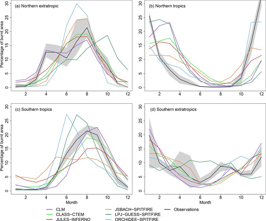
S. Hantson et al.: FireMIP model evaluation                                                                                 3301

and diagnosis of interactions between simulated vegetation          tively strong fire suppression associated with human activ-
and fire.                                                           ities (Teckentrup et al., 2019), were able to reproduce the
   Systematic model evaluation can also serve another pur-          emergent relationship with human population density. How-
pose. The analysis of future climate and climate impacts            ever, the treatment of the anthropogenic influence on burnt
is often based on results from climate and impact model             area has been identified as a weakness in the FireMIP mod-
ensembles (e.g. Kirtman et al., 2013; Collins et al., 2013;         els (Andela et al., 2017; Teckentrup et al., 2019; Li et al.,
Warszawski et al., 2013), and these ensembles are also be-          2019; Forkel et al., 2019a), mainly due to a lack of process
ing used as a basis for impact assessments (e.g. Settele et al.,    understanding.
2014; Hoegh-Guldberg et al., 2019). However, there is in-              In this paper, we focus on quantitative evaluation of model
creasing dissatisfaction with the idea of using the average be-     performance using the baseline historical simulation and
haviour of model ensembles without accounting for the fact          a range of vegetation and fire observational datasets. We
that some models are less reliable than others (Giorgi and          use the vegetation-model evaluation framework described by
Mearns, 2002; Knutti, 2010; Parker et al., 2013), and many          Kelley et al. (2013), with an extended set of data targets to
have called for “the end of model democracy” (e.g. Held,            quantify the fire and vegetation properties and their uncer-
2005; Knutti, 2010). Although there is still considerable dis-      tainties. We identify (i) common weaknesses of the current
cussion about how to constrain models using observations,           generation of global fire-vegetation models and (ii) factors
and then how to combine and possibly weight models de-              causing differences between the models and (iii) discuss the
pending on their overall performance or performance against         implications for future model development.
a minimum set of specific criteria (e.g. Eyring et al., 2005;
Tebaldi et al., 2005; Gleckler et al., 2008; Weigel et al., 2008;
Santer et al., 2009; Parker, 2013; Abramowitz et al., 2019), it     2     Methods
is clear that results from systematic evaluations are central to
                                                                    2.1    Model simulations
this process.
   A number of papers have examined specific aspects of the         The baseline FireMIP simulation is a transient experiment
FireMIP baseline simulations. Andela et al. (2017) showed           starting in 1700 CE and continuing to 2013 (see Rabin et
that the FireMIP models do not reproduce the decrease in            al., 2017, for description of the modelling protocol and the
global burnt area over the past 2 decades inferred from anal-       sources of the input data for the experiments). Models were
ysis of version 4s of the Global Fire Emission Database             spun up until carbon stocks were in equilibrium for 1700 CE
(GFED4s) data product. In fact, four of the models show             conditions (equilibrium was defined as < 1 % change over a
an increase in burnt area over the period 1997–2014. Al-            50-year time period for the slowest carbon pool in each grid
though the remaining five models show a decrease, their             cell) using land use and population density for 1700 CE, CO2
mean decrease is only about one-tenth of the observed rate          concentration for 1750 CE, and recycling climate and light-
(−0.13 ± 0.56 % yr−1 , compared to the observed trend of            ning data from 1901 to 1920 CE. Although the experiment
−1.09 ± 0.61 % yr−1 ). However, the observed global decline         is fully transient after 1700 CE, annually varying values of
of burnt area derived from satellite data is strongly dominated     all these forcings are not available until after 1900 CE. Cli-
by African savanna ecosystems; the spatial pattern of trends        mate, land use, population and lightning were regridded to
is very heterogeneous, and the satellite record is still very       the native grid of each model. Global fire–vegetation mod-
short, which raises issues about the robustness of these trends     els ran with either dynamic or prescribed natural vegetation
(Forkel et al., 2019b). Li et al. (2019) compared modelled          (Table 1), but all used observed time-evolving cropland and
and satellite-based fire emissions and concluded that most          pasture (if simulated) distribution.
FireMIP models fall within the current range of observational          Nine coupled fire–vegetation models have performed the
uncertainty. Forkel et al. (2019a) compared the emergent re-        FireMIP baseline experiments. The models differ in com-
lationships between burnt area and multiple potential drivers       plexity, representation of human impact and vegetation dy-
of fire behaviour, including human caused ones, as seen in          namics, and spatial and temporal resolution (Table 1). A
observations and the FireMIP models. They show that, al-            detailed description of each model is given in Rabin et
though all of the models capture the observed emergent rela-        al. (2017). Most of the models ran simulations for the full
tionships with climate variables, there are large differences in    period 1700–2013, but CLASS–CTEM, JULES–INFERNO,
their ability to capture vegetation-related relationships. This     MC2 and CLM simulated 1861–2013, 1700–2012, 1902–
is underpinned by a regional study using the FireMIP mod-           2009 and 1850–2013 respectively. This slight deviation from
els over China that showed that there are large differences in      the protocol does not affect the results of all but one model
simulated vegetation biomass, hence in fuel loads, between          presented here as we only analyse data for the present-day
the models (Song et al., 2020). These results make a focus          period (2002–2012). For MC2, the 2002–2009 time period
on benchmarking both simulated fire and vegetation partic-          was used for analysis, which might influence the results for
ularly pertinent. Forkel et al. (2019a) showed that some of         this model.
the FireMIP models, specifically those that include a rela-

https://doi.org/10.5194/gmd-13-3299-2020                                              Geosci. Model Dev., 13, 3299–3318, 2020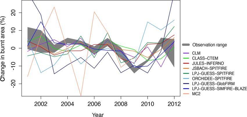
3302                                                                                            S. Hantson et al.: FireMIP model evaluation

Table 1. Brief description of the global fire models that ran the FireMIP baseline experiments. Process indicates models which explicitly
simulate ignitions and fire spread. A detailed overview can be found in Rabin et al. (2017).

 Model                        Dynamic                          Fire model   Human suppression    Spatial resolution   Temporal      Reference
                              biogeography                     type         of fire spread/            (long × lat)   resolution
                                                                            burnt area
 CLM                          No                               Process      Yes                        2.5◦ × 1.9◦    Half hourly   Li et al. (2013)
 CLASS–CTEM                   No                               Process      Yes                 2.8125◦ × 2.8125◦     Daily         Melton and Arora (2016)
 JULES–INFERNO                Yes, but without fire feedback   Empirical    No                    1.875◦ × 1.245◦     Half hourly   Mangeon et al. (2016)
 JSBACH–SPITFIRE              No                               Process      Yes                   1.875◦ × 1.875◦     Daily         Lasslop et al. (2014)
 LPJ–GUESS–SPITFIRE           Yes                              Process      No                         0.5◦ × 0.5◦    Daily         Lehsten et al. (2009)
 LPJ–GUESS–GlobFIRM           Yes                              Empirical    No                         0.5◦ × 0.5◦    Annual        Smith et al. (2014)
 LPJ–GUESS–SIMFIRE–BLAZE      Yes                              Empirical    Yes                        0.5◦ × 0.5◦    Annual        Knorr et al. (2016)
 MC2                          Yes                              Process      No                         0.5◦ × 0.5◦    Monthly       Bachelet et al. (2015)
 ORCHIDEE–SPITFIRE            No                               Process      No                         0.5◦ × 0.5◦    Daily         Yue et al. (2014)

2.2    Benchmarking reference datasets                                            – Burnt area
                                                                                     Five global burnt fraction products were used in this
Model performance was evaluated using site-based and re-
                                                                                     study (Fig. S1). We used the fourth version of the
motely sensed global datasets of fire occurrence, fire-related
                                                                                     Global Fire Emissions Database (GFED4) for 1997-
emissions and vegetation properties (Fig. 1; Fig. S1 in the
                                                                                     2013, which uses the MCD64 burnt area MODIS-based
Supplement). We include vegetation variables (e.g. gross
                                                                                     product in combination with an empirical estimation of
primary productivity, GPP; net primary productivity, NPP;
                                                                                     burnt area based on thermal anomalies when MODIS
biomass; and leaf area index, LAI) because previous analy-
                                                                                     data were unavailable (Giglio et al., 2013). We also in-
ses have indicated that they are critical for simulating fire oc-
                                                                                     cluded a version where the MCD64 burnt area prod-
currence and behaviour (Forkel et al., 2019a; Teckentrup et
                                                                                     uct was merged with the small fire detection approach
al., 2019), and there are global datasets available. We did not
                                                                                     developed by Randerson et al. (2012; GFED4s). The
consider parameters such as soil or litter moisture because,
                                                                                     third dataset is the MODIS burnt area product MCD45,
although these may have an important influence on fire be-
                                                                                     which is the only burnt area product not using MODIS
haviour, globally comprehensive datasets are not available.
                                                                                     thermal anomalies within its burnt area detection al-
All datasets are plotted in Fig. S1. We used multiple datasets
                                                                                     gorithm (2002–2013) (Roy et al., 2008). The fourth is
as targets for variables where they were available in order to
                                                                                     the FireCCIv4.0 dataset based on MERIS satellite data
take into account observational uncertainty.
                                                                                     (Alonso-Canas and Chuvieco, 2015), available for the
   Ideally, model benchmarking should take account of un-
                                                                                     period 2005–2011. The fifth is the FireCCI5.1 dataset
certainties in the observations. However, observational un-
                                                                                     based on MODIS 250m imagery (Chuvieco et al.,
certainties are not reported for most of the datasets used here
                                                                                     2018).
(e.g. vegetation carbon). While it would in principle be pos-
sible to include uncertainty for example by down-weighting                        – Fire emissions.
less reliable datasets (e.g. Collier et al., 2018), determin-
                                                                                     Carbon emission by fires is estimated within the Global
ing the merits of the methods used to obtain observational
                                                                                     Fire Assimilation System (GFAS) based on satellite-
data is rather subjective, and there is no agreement as to
                                                                                     retrieved fire radiative power (FRP) (Kaiser et al.,
which is more reliable if multiple reference datasets exist
                                                                                     2012). Here we use the global GFAS data for the period
for the same variable (e.g. burnt area). Furthermore, some of
                                                                                     2000–2013.
the datasets (e.g. emissions) involve modelled relationships;
there has been little assessment of the impact of the choice of                   – Fire size and numbers.
model on the resultant uncertainty in emission estimates (e.g.
                                                                                     Estimates on mean size and number of fires can be pro-
Kaiser et al., 2012). While we use multiple datasets when
                                                                                     duced using a flood-filling algorithm to extract individ-
available (e.g. for burnt area, where there are extremely large
                                                                                     ual fires (Archibald et al., 2013). Here we use the data
differences between the products and they may all underesti-
                                                                                     as produced by Hantson et al. (2015) from the MCD45
mate the actual burnt area; Roteta et al., 2019), in an attempt
                                                                                     global burnt area product (Roy et al., 2008). Only large
to integrate observational uncertainty in our evaluations, it
                                                                                     fires ≥ 25 ha (1 MODIS pixel) are detected, with a con-
seems premature to incorporate uncertainty in the benchmark
                                                                                     siderable underestimation of fires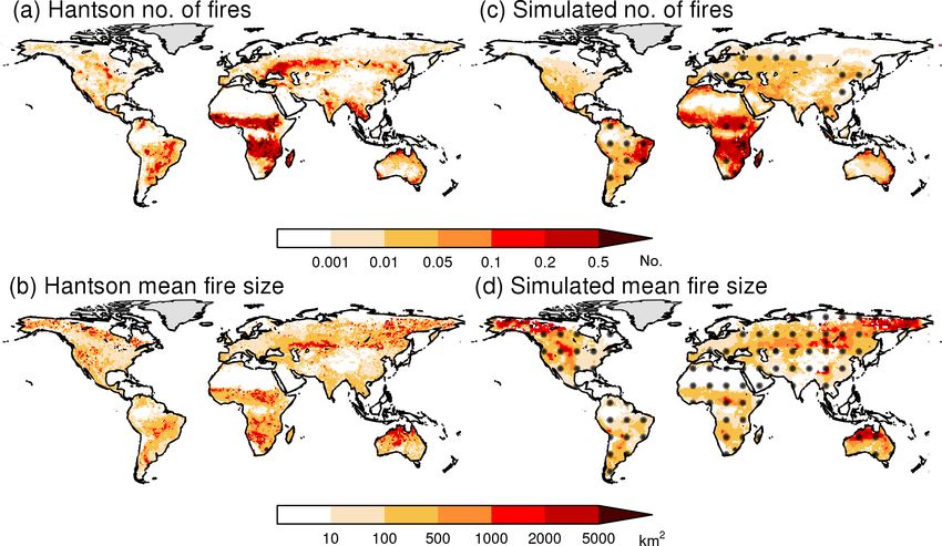
S. Hantson et al.: FireMIP model evaluation                                                                                3303

  – Vegetation productivity.                                       value of the observations and a “random” model produced
      We use multiple datasets for vegetation productivity,        by bootstrap resampling of the observations.
      both measurements from site locations and global up-            Normalized mean error (NME) was selected over other
      scaled estimates. The site-level GPP dataset is from         metrics (e.g. RMSE) as these normalized scores allow for di-
      Luyssaert et al. (2007), and the site-level NPP combines     rect comparison in performance between variables with dif-
      these data with data from the Ecosystem Model-Data           ferent units (Kelley et al., 2013). NME is more appropri-
      Intercomparison (EMDI; Olson et al., 2001) databases.        ate for variables which do not follow a normal distribution,
      Sites from managed or disturbed environments were not        and it has therefore been used as the standard metric to as-
      used. A recent compilation of NPP site-level estimates       sess global fire model performance (e.g. Kloster and Lasslop,
      was compiled by Michaletz et al. (2014). The mean of         2017; Kelley et al., 2019; Boer et al., 2019). NME is defined
      observations was taken when more than one measure-           as
      ment was available within a 0.5◦ grid cell. We also use
                                                                            P
                                                                                Ai |obsi − simi |
      upscaled FLUXNET GPP data (Jung et al., 2017; Tra-           NME = P                        ,                           (1)
                                                                                Ai obsi − obs
      montana et al., 2016). Kelley et al. (2013) showed that
      the spreading of data between FLUXNET site observa-          where the difference between observations (obs) and simu-
      tions in such upscaling artificially improved model per-     lation (sim) are summed over all cells (i) weighted by cell
      formance, probably because it used similar input data        area (Ai ) and normalized by the average distance from the
      and methods, which might emulate functional relation-        mean of the observations (obs). Since NME is proportional
      ships used within DGVMs. Hence scores obtained by            to mean absolute errors, the smaller the NME value, the bet-
      Jung should not be interpreted as true “benchmarking         ter the model performance. A score of 0 represents a perfect
      scores” but could help inform differences between mod-       match to observations. NME has no upper bound.
      els in relation to scores obtained from other compar-           NME comparisons were conducted in three steps follow-
      isons like burnt area (See Fig. S1).                         ing Kelley et al. (2013):
  – Carbon in vegetation.                                            – Step 1 is as described above.
      A global dataset on aboveground vegetation biomass
                                                                     – Step 2 is with obsi and simi replaced with the difference
      was recently produced by combining two existing
                                                                       between observation or simulation and their respective
      datasets – Saatchi et al. (2011) and Baccini et al. (2012)
                                                                       means, i.e. xi → xi − x̄, removing systematic bias and
      – using a reference dataset of field observations and es-
                                                                       describe the performance of the model around the mean.
      timates (Avitabile et al., 2016). However, this dataset
      only considers woody biomass, and to be able to analyse        – Step 3 is where obsi and simi from step 2 were divided
      vegetation carbon also for areas without tree cover we           by the mean deviation, i.e. xi → xi / |xi |. This removed
      used the dataset generated by Carvalhais et al. (2014),          the influence of bias in the variability and described the
      which combined the Saatchi et al. (2011) and Thurner             models ability to reproduce the spatial pattern in burnt
      et al. (2014) biomass datasets while providing a best es-        area.
      timate for herbaceous biomass.
                                                                   To limit the impact of observational uncertainties in the ref-
  – Leaf area index (LAI).                                         erence datasets on the comparisons and as NME can be sen-
      We use the MODIS LAI product MCD15, which gives              sitive to the simulated magnitude of the variable, we mainly
      global LAI values each 8 d (Myneni et al., 2002) and         focus on benchmarking results after removing the influence
      the LAI dataset produced based on AVHRR (Claverie            of biases in the mean and variance (step 3). However, com-
      et al., 2016). The mean LAI over the period 2001–2013        parisons of steps 1 and 2 are given in Table S1 in the Supple-
      is used for benchmarking.                                    ment.
                                                                      To assess a model’s ability to reproduce seasonal patterns
2.3   Model evaluation and benchmarking                            in a variable, we focused on seasonal concentration (roughly
                                                                   equivalent to the inverse of season length) and seasonal phase
We adopted the metrics and comparison approach specified           (or timing) comparisons from Kelley et al. (2013). This uses
by Kelley et al. (2013) as it provides a comprehensive scheme      the mean seasonal “vector” for each observed and simulated
for the evaluation of vegetation models. This protocol pro-        location based on the monthly distribution of the variable
vides specifically designed metrics to quantify model perfor-      through the year, whereby each month, m, is represented by
mance in terms of annual-average, seasonal and interannual         a vector in the complex plane whose direction (θm ) corre-
variability against a range of global datasets, allowing the       sponds to the time of year, and length corresponds to the
impact of spatial and temporal biases in means and variabil-       magnitude of the variable for that month as follows:
ity to be assessed separately. The derived model scores were
compared to scores based on the temporal or spatial mean           θm = 2 · π · (m − 1)/12.                                   (2)

https://doi.org/10.5194/gmd-13-3299-2020                                             Geosci. Model Dev., 13, 3299–3318, 2020
3304 S. Hantson et al.: FireMIP model evaluation
A mean vector L is the average of the real (Lx ) and imagi- 0.5◦ grid. Although some models were run at a coarser reso-
nary (Ly ) parts of the 12 vectors (xm ). lution, the spatial resolution at which the benchmarking was
performed had only a limited impact on the scores (Fig. S2),
Lx = 6m xm · cos (θm ) which does not affect conclusions drawn here. Each model
Ly = 6m xm · sin (θm ) (3) was compared to each reference dataset except in the few
cases where the appropriate model output was not provided
The mean vector length by the annual average describes the (e.g. LAI in ORCHIDEE, GPP in MC2). Only the models
seasonal concentration (C) of the variable, while its direction which incorporate the SPITFIRE fire module provided fire
(P ) describes seasonal timing (phase) as follows: size and number results.
q
L2x + L2y
C= (4) 3 Results
6m x m
Lx 3.1 Modern-day model performance: burnt area and
P = arctan . (5)
Ly fire emissions
If the variable in a given cell is concentrated all in 1 month, The simulated modern (2002–2012) total global annual burnt
then, C is equal to 1, and P corresponds to that month. If area is between 39 and 536 Mha (Table 2). Most of the
burnt area is evenly spread throughout the year, then con- FireMIP models are within the range of burnt area esti-
centration is zero, and phase is undefined. Where the phase mated by the individual remotely sensed products (354 to
of a cell is undefined in either observations or simulation, 468 Mha yr−1 ). LPJ–GUESS–GlobFIRM and MC2 simulate
then it was not used in the comparison. Likewise, if a cell much less burnt area than that shown by any of the prod-
has zero annual average burnt area for either observations or ucts, and CLASS–CTEM simulates more than shown by any
simulation, then that cell is not included in the comparisons. of the products. However, use of the range of the remotely
Concentration was compared using NME step 1. Phase was sensed estimates may not be a sufficient measure of the un-
compared using the mean phase difference metric (MPD): certainty in burnt area because four of them are derived from
1 the same active fire product (Forkel et al., 2019a), and re-
MPD = 6i Ai · arcos cos Psim,i − Pobs,i /6i Ai . (6) cent work suggests that they may all underestimate burnt area
π
(Roteta et al., 2019). Thus, we cannot definitively say that the
MPD represents the average timing error, as a proportion of apparent overestimation by CLASS–CTEM is unrealistic.
the maximum phase mismatch (6 months). With the exception of MC2 and LPJ–GUESS–GlobFIRM,
Seasonality metrics could not be calculated for three mod- the models realistically capture the spatial patterns in burnt
els (LPJ–GUESS–GlobFIRM, LPJ–GUESS–SIMFIRE– area (Figs. 1 and 2) and perform better than either of the null
BLAZE, MC2), either because they do not simulate the models irrespective of the reference burnt area dataset (Ta-
seasonal cycle or because they did not provide these outputs. ble 3). CLM (NME: 0.63–0.80) and ORCHIDEE–SPITFIRE
We did not use FireCC4.0 to assess seasonality or interan- (0.70–0.73) are the best performing models. All the FireMIP
nual variability (IAV) in burnt area because it has a much models correctly simulate most burnt area in the tropics (24–
shorter times series than the other burnt area products. 466 Mha yr−1 ) compared to observed values in the range of
Model scores are interpreted by comparing them to two 312–426 Mha yr−1 (Table 2). The simulated contribution of
null models (Kelley et al., 2013). The “mean” null model tropical fires to global burnt area is in the range of 56 % to
compares each benchmark dataset to a dataset of the same 92 %, with all models except ORCHIDEE–SPITFIRE simu-
size created using the mean value of all the observations. The lating a lower fraction than observed (89 %–93 %). This fol-
mean null model for NME always has a value of 1 because lows from FireMIP models tending to underestimate burnt
the metric is normalized by the mean difference. The mean area in Africa and Australia, although burnt area in South
null model for MPD is based on the mean direction across all American savannas is usually overestimated (Table 2). All of
observations, and therefore the value can vary and is always the FireMIP models, except LPJ–GUESS–GlobFIRM, cap-
less than 1. The “randomly resampled” null model com- ture a belt of high burnt area in central Eurasia. However, the
pares the benchmark dataset to these observations resampled models overestimate burnt area across the extratropics on av-
1000 times without replacement (Table 3). The randomly re- erage by 180 % to 304 %, depending on the reference burnt
sampled null model is normally worse than the mean null area dataset. This overestimation largely reflects the fact that
model for NME comparisons. For MPD, the mean will be the simulated burnt area over the Mediterranean basin and
better than the random null model when most grid cells show western USA is too large (Table 2, Fig. 2).
the same phase. The FireMIP models that include a subannual time
For comparison and application of the benchmark metrics, step for fire calculations (CLM, CLASS–CTEM, JULES–
all the target datasets and model outputs were resampled to a INFERNO, JSBACH–SPITFIRE, LPJ–GUESS–SPITFIRE,
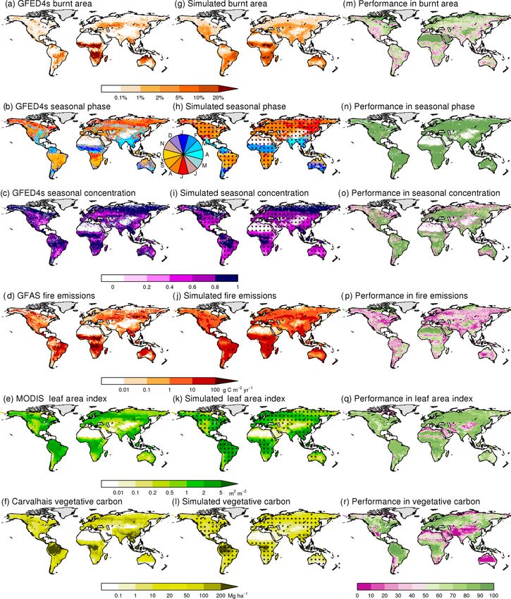
Geosci. Model Dev., 13, 3299–3318, 2020 https://doi.org/10.5194/gmd-13-3299-2020S. Hantson et al.: FireMIP model evaluation 3305 Figure 1. Reference datasets, the mean of all models and the percent of models for which the estimate falls within 50 %–200 % of the (mean) reference data are presented for a set of fire relevant variables. Results for the following variables are given as follows: (a) fraction burnt area, (b) seasonal timing of burnt area (as measured by mean phase), (c) burnt area season length (as measured by seasonal concentration), (d) fire C emissions (g C m−2 yr−1 ), (e) vegetation carbon (Mg ha−1 ) and (f) leaf area index (LAI) (m2 m−2 ). Stippling in the second column indicates where variance between models is less than the FireMIP model ensemble mean. Purple in the third column indicates cell where the majority of the FireMIP models produce poor simulations of the variable, while green areas indicate that the majority of the FireMIP models perform well for that aspect of the fire regime. ORCHIDEE–SPITFIRE) generally reproduce the seasonal- pendent of the reference burnt area dataset. The observations ity of burnt area (Fig. 3), particularly in the tropics. The show a unimodal pattern in burnt area in the tropics, peak- models capture the timing of the peak fire season reasonably ing between November and the end of February in the north- well, with all of the models performing better than mean null ern tropics and between June and the end of October in the model for seasonal phase in burnt area (Table 3). The models southern tropics (Fig. 3). The models also show a unimodal also frequently perform better than the random null model, pattern in both regions. However, all the FireMIP models with all models performing better against GFED4. How- except ORCHIDEE–SPITFIRE show a ∼ 2-month delay in ever, all of the FireMIP models perform worse than mean peak burnt area in the northern tropics, and the period with null model for seasonal concentration of burnt area, inde- high burnt area is also less concentrated than observed. Some https://doi.org/10.5194/gmd-13-3299-2020 Geosci. Model Dev., 13, 3299–3318, 2020
3306 S. Hantson et al.: FireMIP model evaluation
Table 2. Simulated and observed burnt area (Mha) for the period 2002–2012 for the globe and for key regions including the northern
extratropics (NET; >30◦ N), the southern extratropics (SET; > 30◦ S), the tropics (30◦ N–30◦ S), the savanna regions of Africa (18◦ W–40◦ E,
13◦ N–20◦ S), the savanna region of South America (42–68◦ W, 9–25◦ S), the Australian savanna (120–155◦ E, 11–20◦ S), the agricultural
band of central Eurasia (30–85◦ E, 50–58◦ N), the Mediterranean basin (10◦ W–37◦ E, 31–44◦ N) and the western USA (100–125◦ W, 31–
43◦ N). Data availability for FireCCI40 is limited to 2005–2011 and for MC2 to 2002–2009.
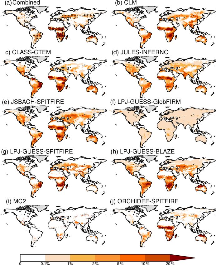
Global NET Tropics SET S American African Australian Central Mediterranean Western
savanna savanna savanna Eurasia basin USA
GFED4s 468 39 426 4 18 295 35 8.5 1.3 1.0
GFED4 349 27 319 3 14 218 34 5.2 0.8 0.9
MCD45 348 33 312 4 13 232 25 7.0 2.0 0.9
FireCCI40 345 23 320 2 8 237 25 6.8 1.1 0.8
FireCCI51 387 37 347 3 14 230 38 10.2 1.3 1.1
CLM 454 77 362 15 36 194 15 7.9 9.3 3.4
CLASS–CTEM 536 41 466 28 46 172 20 2.0 4.3 9.5
JULES–INFERNO 381 76 292 13 26 128 23 5.0 11.0 7.7
JSBACH–SPITFIRE 457 114 318 25 21 166 17 15.5 9.5 9.7
LPJ–GUESS–GlobFIRM 39 14 24 1 3 7 3 0.6 0.6 0.5
LPJ–GUESS–SPITFIRE 393 99 280 14 51 135 2.8 12.5 14.5 6.1
LPJ–GUESS–SIMFIRE–BLAZE 482 86 381 15 72 146 27 3.4 7.9 14.9
MC2 97 40 54 3 2 17 2 0.9 5.0 2.2
ORCHIDEE–SPITFIRE 471 16 435 19 13 246 81 2.4 2.4 0.3
models (ORCHIDEE–SPITFIRE, LPJ–GUESS–SPITFIRE)
estimate peak burnt area ∼ 1–2 months too early in the
southern tropics, while others simulate a peak ∼ 1 month
too late (JULES–INFERNO, CLM, CLASS–CTEM) or have
a less concentrated peak (JSBACH–SPITFIRE, JULES–
INFERNO) than observed. The seasonality of burnt area
in the northern extratropics shows a peak in spring and a
second peak in summer. Only CLM reproduces this double
peak, while all of the other FireMIP models show a single
summer peak. Most of the models simulate the timing of
the summer peak well. The only exception is LPJ–GUESS–
SPITFIRE, which simulates the peak ∼ 2–3 months too late.
The observations show no clear seasonal pattern in burnt area
over the southern extratropics, although the most prominent
peak occurs in December and January. All the FireMIP mod-
els, except LPJ–GUESS–SPITFIRE, reproduce this midsum-
mer peak. LPJ–GUESS–SPITFIRE shows little seasonality
in burnt area in this region.
The FireMIP models have problems representing IAV in
global burnt area, with some models (CLASS–CTEM, MC2)
worse than the random model and most models performing
worse than the mean for most of the target datasets (Table 3).
However, there is considerable uncertainty in the observed
IAV in burnt area (Fig. 4), and the scores are therefore de-
pendent on the reference dataset considered, with generally
worse scores for FireCCI5.1 and GFED4s compared to the
Figure 2. Simulated versus observed burnt fraction (% yr−1 ) for other datasets. Observational uncertainty is most probably
the present day (2002–2012), where “combined” indicates the mean
underestimated as the burnt area products are not indepen-
of the different burnt area datasets considered. Stippling indicates
dent, since they all rely on MODIS satellite imagery. Despite
where variance between burnt area datasets is less than the observed
ensemble mean. the failure to reproduce IAV in general, most of the models
show higher burnt area in the early 2000s and a low in 2009–
2010 after which burnt area increased again (Fig. 4).
Geosci. Model Dev., 13, 3299–3318, 2020 https://doi.org/10.5194/gmd-13-3299-2020S. Hantson et al.: FireMIP model evaluation 3307 Table 3. Benchmarking scores after removing the influence of differences in the mean and variance for each individual global fire model for key fire and vegetation variables. A lower score is “better”, with a perfect score equal to 0. The full table with all benchmarking scores is presented in Table S1 in the Supplement. LPJ–G: LPJ–GUESS. Cell are coloured blue if the benchmarking score is lower than both null models, yellow if lower than 1 null model and red when higher than both null models. https://doi.org/10.5194/gmd-13-3299-2020 Geosci. Model Dev., 13, 3299–3318, 2020
3308                                                                           S. Hantson et al.: FireMIP model evaluation

   The spatial patterns in simulated fire-related carbon emis-   trated across the northern extratropics. Thus, the better match
sions are in line with the reference data, with most FireMIP     between the FireMIP models and the upscaled FLUXNET
models except LPJ–GUESS–GlobFIRM, MC2 and LPJ–                   dataset may reflect the broader spatial coverage or the fact
GUESS–SPITFIRE performing better than the mean null              that climate and land-cover data are used for upscaling.
model. CLM, JULES–INFERNO and JSBACH–SPITFIRE                       Only the upscaled FLUXNET data provide monthly data
are the best performing models with NME scores < 0.8. Sea-       and can thus be used to assess GPP seasonality. The FireMIP
sonality in fire emissions mimics the results for burnt area     models are able to represent the seasonal peak timing in GPP,
with good scores for seasonal phase, but all models perform      with all models performing better than the mean and random
worse than the mean null model for seasonal concentration.       null models. However, models have difficulty in representing
CLM is the only FireMIP model to explicitly include peat-        the length of the growing season, with the scores for seasonal
land, cropland and deforestation fires, which contribute 3 %,    concentration in GPP (1.08–1.23) above the mean null model
3 % and 20 % respectively of the global total emissions an-      but below the random null model for all FireMIP models.
nually (van der Werf et al., 2010), but it nevertheless does        Model performance is better for site-level NPP than site-
not perform better than JULES–INFERNO and JSBACH–                level GPP. All of the FireMIP models perform better than
SPITFIRE in representing the spatial pattern of fire carbon      the mean null model, independent of the choice of refer-
emissions.                                                       ence dataset (Table 3), except for CLASS–CTEM against the
   Only three models (JSBACH–SPITFIRE, LPJ–GUESS–                Luyssaert dataset. JULES–INFERNO, JSBACH–SPITFIRE
SPITFIRE, ORCHIDEE–SPITFIRE) provided information                and MC2 are the best-performing models.
about simulated numbers and size of individual fires. All           The FireMIP models generally capture the spatial pattern
three models performed better than the mean null model in        in LAI, with all models performing better than the mean null
representing the spatial pattern in number of fires but worse    model (0.44–0.81), independent of the reference dataset con-
than the mean model for fire size (Table 3). While the spatial   sidered. JULES–INFERNO has the best score for both refer-
pattern in simulated fire number is in agreement with obser-     ence datasets. Although the overall global pattern in LAI is
vations over large parts of the globe, models tend to over-      well represented in all the FireMIP models, they have more
estimate fire numbers in dryland areas such as Mexico and        trouble representing LAI in agricultural areas such as the
the Mediterranean basin (Fig. 5). None of the three models       central USA or areas with low LAI such as drylands and
simulate cropland fires, and so they do not capture the high     mountain areas (Fig. 1).
number of cropland fires (Hall et al., 2016) in central Eura-       The FireMIP models perform well in representing the spa-
sia (Table 2). Models simulate smaller fires than observed       tial pattern carbon in vegetation (Table 3). All nine models
in areas where burnt area is large and where models tend to      perform better than the mean null model, independent of ref-
underestimate burnt area, especially in the African savanna      erence dataset, with ORCHIDEE–SPITFIRE having the best
regions (Fig. 5).                                                scores. Generally, the models are able to simulate carbon in
                                                                 tropical vegetation and the forested regions in the temperate
3.2    Present-day model performance: vegetation                 and boreal region reasonably well but struggle across most
       properties                                                dryland systems (Fig. 1).

Fire spread and hence burnt area is strongly influenced          3.3   Overall assessment
by fuel availability, which in turn is affected by veg-
etation primary production and biomass. Simulated spa-           Our evaluation suggests that LPJ–GUESS–GlobFIRM and
tial patterns of GPP compare well with estimates of GPP          MC2 produce substantially poorer simulations of burnt area
upscaled from FLUXNET data (Jung et al., 2017), with             and its interannual variability than other models in the
scores (0.39–0.67) considerably better than both null mod-       FireMIP ensemble. These are both older models, developed
els. However, performance against site-based estimates of        before the availability of global burnt area products (in the
GPP (Luyssaert et al., 2007) are considerably poorer (1.09–      case of LPJ–GUESS–GlobFIRM) or calibrated regionally
1.49) and worse than the mean null model. Only LPJ–              and not designed to run at global scale (MC2). While the
GUESS–SPITFIRE, LPJ–GUESS–SIMFIRE–BLAZE and                      other models perform better in simulating fire properties,
ORCHIDEE–SPITFIRE perform better than the random null            there is no single model that outperforms other models across
model. There is no clear relationship between model scores       the full range of fire and vegetation benchmarks examined
for the two datasets; models performing better when com-         here. Model structure does not explain the differences in
pared to the Jung dataset do not necessarily show a higher       model performance. Process-based fire models (see Table 1)
score when compared to the Luyssaert GPP dataset. The two        appear to be slightly better able to represent the spatial pat-
GPP datasets are very different. The upscaled FLUXNET            tern in burnt area than empirical models (mean score of 0.87
dataset is a modelled product but has global coverage (see       and 0.94 respectively), but this difference is largely the result
Methods), while the Luyssaert dataset has local measure-         of including GlobFIRM in the empirical model ensemble; re-
ments but only at a limited number of sites, largely concen-     moving this model results in a mean score of 0.87 for these

Geosci. Model Dev., 13, 3299–3318, 2020                                           https://doi.org/10.5194/gmd-13-3299-2020
S. Hantson et al.: FireMIP model evaluation 3309
Figure 3. Simulated and observed seasonality (2002–2012) of burnt area (% of annual burnt area per month) for (a) northern extratropics
(> 30◦ N), (b) northern tropics (0–30◦ N), (c) southern tropics (0–30◦ S) and (d) southern extratropics (> 30◦ S). The mean of all the remotely
sensed burnt area datasets is shown as a black line, with the minimum and maximum range shown in light grey.
is no difference in the performance of process-based and em-
pirical models with respect to IAV in burnt area, seasonal
phase in burnt area or fire emissions.
The FireMIP simulations include three models in which
versions of the same process-based fire module (SPITFIRE)
are coupled to different vegetation models. These three mod-
els produce a wide range of benchmarking scores for burnt
area, with mean benchmarking scores of 0.79, 0.85 and 0.72
for JSBACH, LPJ–GUESS and ORCHIDEE respectively.
There are also large differences between these models in
terms of other aspects of the fire regime (Table 3). As there
Figure 4. The range in interannual variability in burnt area for the
are only moderate differences between the different SPIT-
years 2001–2012 for all models and burnt area datasets which span
the entire time period (GFED4, GFED4s, MCD45, FireCCI51). Re- FIRE implementations (Rabin et al., 2017), this suggests that
sults from the individual FireMIP models, as well as the observa- the overall difference between the models reflect interactions
tional minimum-maximum values, are plotted. between the fire and vegetation modules.
Models using prescribed vegetation biogeography (CLM,
CLASS–CTEM, JSBACH–SPITFIRE, ORCHIDEE–
SPITFIRE) represent the spatial pattern of burnt area better
models. The intermodel spread in scores within each group than models with dynamic vegetation (JULES–INFERNO,
is much larger than the difference between the two types of LPJ–GUESS–SPITFIRE, LPJ–GUESS–GlobFIRM, LPJ–
model. Only one empirical model simulates fire seasonality, GUESS–SIMFIRE–BLAZE, MC2), with respective mean
but this model performs worse than each of the process-based benchmarking scores across all burnt area datasets of
models, independent of reference dataset considered. There
https://doi.org/10.5194/gmd-13-3299-2020 Geosci. Model Dev., 13, 3299–3318, 20203310 S. Hantson et al.: FireMIP model evaluation
0.79 and 0.97. This difference is still present even when CLM is the only model that incorporates cropland fires
LPJ–GUESS–GlobFIRM and MC2 are not included (0.90). (Table 1), and it is also the only model which captures the
It seems likely that models using prescribed vegetation spring peak in burnt area in the northern extratropics asso-
biogeography have a better representation of fuel loads ciated with crop fires (e.g. Le Page et al., 2010; Magi et al.,
and flammability. This can also partially be seen in the 2012; Hall et al., 2016). This might also contribute to the
positive relationship between the benchmarking scores of good overall score of CLM for spatial pattern of burnt area.
vegetation carbon and burnt area spatial patterns for at least
the GFED4, FireCCI4.0 and FireCCI5.1 burnt area reference
datasets (mean of R 2 = 0.31; range of 0.19–0.38). Areas 4 Discussion
where the FireMIP models represent vegetation carbon
poorly coincide with some of the regions where models have There are large differences in the total burnt area between the
trouble representing the spatial pattern of burnt area such as FireMIP models, with two models (LPJ–GUESS–GlobFIRM
dryland regions (Fig. 1). Although there is no relationship and MC2) falling well outside the observed range in burnt
between GPP/NPP and burnt area benchmarking scores, area for the recent period. In the case of LPJ–GUESS–
there is a positive relationship between simulated burnt area GlobFIRM, this is because GlobFIRM was developed before
scores and the seasonal concentration of GPP (R 2 = 0.30– global burnt area products were available, resulting in a gen-
0.84) and, to a lesser extent, the seasonal phase of GPP eral poor performance (Kloster and Lasslop, 2017), in com-
(R 2 = 0.09–0.24). Models which correctly predict the bination with the fact that structural changes were made to
seasonal pattern of GPP/NPP, which has a strong influence the vegetation model without a commensurate development
on the availability of fuel, are more likely to predict the burnt of the fire module. In the case of MC2, this probably reflects
area correctly. This supports the idea that the seasonality of the fact that MC2 was developed for regional applications
vegetation production and senescence, is among the chief but was applied globally here without any refinement of the
drivers of the interactions between vegetation and fire within fire model. The other FireMIP models used the burned area
each model. However, since fires combust some of the datasets to develop and tune their models. They therefore
vegetation and hence reduce fuel loads, fire occurrence also capture the global spatial patterns of burnt area reasonably
influences the seasonality in vegetation productivity. This well, although no model simulates the very high burnt area
may partly explain the varying strength of the correlations in Africa and Australia causing a general underestimation of
between the seasonal concentration and phase and the burnt area in tropical regions and overestimation in extrat-
burnt area. Although both GPP/NPP and burnt area are ropical regions. The analysis of a limited number of models
affected by climate conditions, the emergent relationships suggests that process-based fire models do not simulate the
between simulated and observed climate and burnt area spatial patterns in fire size well (Table 3). In particular they
are generally similar across the FireMIP models (Forkel fail to represent fire size in tropical savannas (Fig. 5), most
et al., 2019), whereas the emergent relationships between probably because they assume a fixed maximum fire duration
vegetation properties and burnt area are much less so. This of less than 1 d (Hantson et al., 2016) while savanna fires are
indicates that fire models could be improved by improving often very long-lived (e.g. Andela et al., 2019). Our results
the simulated fuel availability by a better representation of suggest that process-based fire models could be improved by
the seasonality of vegetation production and senescence. a better representation of fire duration. Although none of the
Fire carbon emission benchmarking scores are strongly re- FireMIP models simulate multiday fires, there are fire models
lated to the burnt area performance (R 2 > 0.85 for GFED4s that do (e.g. Pfeiffer et al., 2013; Le Page et al., 2015), which
and MCD45 and > 0.45 for FireCCI4.0 and GFED4). This could therefore provide a template for future model develop-
indicates that simulated burnt area is the main driver of fire ment. New parameterizations would need to incorporate as-
emissions, overriding spatial patterns in fuel availability and pects of natural and anthropogenic landscape fragmentation
consumption. However, the benchmarking scores for the spa- which limit fire growth (e.g. Pfeifer et al., 2013; Le Page et
tial pattern in burnt area are better overall than those for fire al., 2015; Kelley et al., 2019). Indeed, our results show that
carbon emissions. models that include a human limitation on fire growth repre-
Models that explicitly simulate the impact of human sup- sent the global spatial pattern in burnt area and fire size bet-
pression on fire growth or burnt area (CLM, CLASS–CTEM, ter. The recently generated Global Fire Atlas (Andela et al.,
JSBACH–SPITFIRE, LPJ–GUESS–SIMFIRE–BLAZE) are 2019) includes aspects of the fire behaviour (e.g. fire spread
better at representing the spatial pattern in burnt area com- rate and duration) that offer new opportunities to examine
pared to models which do not include this effect (0.85 and and parameterize fire.
0.93 respectively). In the case of the three process-based Vegetation type and stocks are input variables for the fire
models (CLM, CLASS–CTEM, JSBACH–SPITFIRE) this is models, influencing fire ignition and spread in the process-
most probably because the spatial pattern in fire size is better based models and determining simulated burnt area in the
represented (Table 3). empirical models. The occurrence of fire can, in turn, af-
fect the vegetation type, simulated vegetation productivity
Geosci. Model Dev., 13, 3299–3318, 2020 https://doi.org/10.5194/gmd-13-3299-2020S. Hantson et al.: FireMIP model evaluation 3311 Figure 5. Reference datasets and mean of three models for number of fires and mean fire size. Model output is adapted so that mean and variance coincide with observations as the total values are not directly comparable. Stippling indicates where variance between models is less than the model ensemble mean. (i.e. GPP, NPP) and hence the amount and seasonality of fuel northern extratropics (e.g. Archibald et al., 2009; Le Page et build-up. Our results indicate that intermodel differences in al., 2010; Magi et al., 2012), where the only model that ex- burnt area are related to differences in simulated vegetation plicitly includes crop fires (CLM) is also the only model that productivity and carbon stocks. Seasonal fuel build-up and shows the bimodal seasonality. Thus, the inclusion of anthro- senescence is an important driver of global burnt area. Fur- pogenic fires could help to improve model simulations. How- thermore, we find that models which are better at represent- ever, this requires a better understanding of how fire is used ing the seasonality of vegetation production are also better for land management under different socioeconomic and cul- at representing the spatial pattern in burnt area. These results tural conditions (Pfeiffer et al., 2013; Li et al., 2013). are consistent with the analysis of emergent relationships in Global interannual variability in burnt area is largely FireMIP models, which shows the need to improve processes driven by drought episodes in high biomass regions and fuel related to plant production and biomass allocation to improve buildup after periods of increased rainfall in dryland areas model performance in simulating burnt area (Forkel et al., (e.g. Chen et al., 2017). Previous analysis has shown that 2019a). While there are spatially explicit global estimates re- the FireMIP models are relatively good at representing emer- garding carbon stocks in live vegetation, there is limited in- gent climate–fire relationships (Forkel et al., 2019a); hence formation about carbon stocks of different fuel types and how it seems plausible that fuel build-up and its effect on subse- these change between seasons and over time (van Leeuwen quent burnt area is not well represented in the models and that et al., 2014; Pettinari and Chuvieco, 2016). Furthermore, fuel this is the reason for the poor simulation of IAV in burnt area. availability could be substantially affected by livestock den- This is in line with our findings and the findings of Forkel et sity and pasture management (Andela et al., 2017). While al. (2019a) that fire models are not sensitive enough to previ- improved representation of land management practices could ous previous-season vegetation productivity. improve the representation of fire, the lack of high-quality The spread in simulated global total fire emissions is even fuel availability data currently limits our ability to constrain larger than for burnt area, but fire emissions largely fol- simulated fuel loads. low the same spatial and temporal patterns as burnt area The FireMIP models generally do not simulate the timing (Fig. 1, Table 3). However, the benchmark scores for emis- of peak fire occurrence accurately and tend to simulate a fire sions are worse than those for burnt area. This reflects the season longer than observed. This might be related to the rep- fact that emissions are the product of both errors in simulated resentation of seasonality in vegetation production and fuel vegetation and burnt area. Furthermore, spatial and tempo- build-up. However, human activities can also change the tim- ral uncertainties in the completeness of biomass combustion ing of fire occurrence (e.g. Le Page et al., 2010; Rabin et al., will affect the emissions. While improvements to vegetation 2015), and so an improved representation of the human influ- and fuel loads are likely to produce more reliable estimates ence on fire occurrence and timing could also help to improve of emissions, an improved representation of the drivers of the simulated fire seasonality. The importance of the anthro- combustion completeness in models will also be required pogenic impact on fire seasonality is especially clear in the for more accurate fire emission estimates. Only one of the https://doi.org/10.5194/gmd-13-3299-2020 Geosci. Model Dev., 13, 3299–3318, 2020
3312                                                                S. Hantson et al.: FireMIP model evaluation

FireMIP models (CLM) includes cropland, peatland and de-
forestation fire explicitly, albeit in a rather simple way. Our
analyses suggest that this does not produce an improvement
in the simulation of either the spatial pattern or timing of car-
bon emissions. However, given that together these fires rep-
resent a substantial proportion of annual carbon emissions, a
focus on developing and testing robust parameterizations for
these largely anthropogenic fires could also help to provide
more accurate fire emission estimates.
   Our analysis demonstrates that benchmarking scores pro-
vide an objective measure of model performance and can be
used to identify models that have a might negative impact on
a multimodel mean and so exclude these from further anal-
ysis (e.g. LPJ–GUESS–GlobFIRM, MC2). At the moment,
a further ranking is more difficult because no model clearly
outperforms all other models. Still, some FireMIP models are
better at representing some aspects of the fire regime com-
pared to others. Hence, when using FireMIP output for future
analyses, one could weigh the different models based on the
score for the variable of interest, thus giving more weight to
models which perform better for these variables.

Geosci. Model Dev., 13, 3299–3318, 2020                               https://doi.org/10.5194/gmd-13-3299-2020
You can also read