The Utrecht Finite Volume Ice-Sheet Model: UFEMISM (version 1.0) - GMD
←
→
Page content transcription
If your browser does not render page correctly, please read the page content below
Geosci. Model Dev., 14, 2443–2470, 2021
https://doi.org/10.5194/gmd-14-2443-2021
© Author(s) 2021. This work is distributed under
the Creative Commons Attribution 4.0 License.

The Utrecht Finite Volume Ice-Sheet Model: UFEMISM
(version 1.0)
Constantijn J. Berends1 , Heiko Goelzer1,2,3 , and Roderik S. W. van de Wal1,4
1 Institutefor Marine and Atmospheric research Utrecht, Utrecht University, Utrecht, 3584 CC, the Netherlands
2 Laboratoire  de Glaciologie, Université Libre de Bruxelles, Brussels, Belgium
3 NORCE Norwegian Research Centre, Bjerknes Centre for Climate Research, Bergen, Norway
4 Faculty of Geosciences, Department of Physical Geography, Utrecht University, Utrecht, the Netherlands

Correspondence: Constantijn J. Berends (c.j.berends@uu.nl) and Roderik van de Wal (r.s.w.vandewal@uu.nl)

Received: 26 August 2020 – Discussion started: 8 September 2020
Revised: 15 March 2021 – Accepted: 29 March 2021 – Published: 5 May 2021

Abstract. Improving our confidence in future projections of       for high resolutions. A simulation of all four continental ice
sea-level rise requires models that can simulate ice-sheet evo-   sheets during an entire 120 kyr glacial cycle, with a 4 km
lution both in the future and in the geological past. A physi-    resolution near the grounding line, is expected to take 100–
cally accurate treatment of large changes in ice-sheet geome-     200 wall clock hours on a 16-core system (1600–3200 core
try requires a proper treatment of processes near the margin,     hours), implying that this model can be feasibly used for
like grounding line dynamics, which in turn requires a high       high-resolution palaeo-ice-sheet simulations.
spatial resolution in that specific region, so that small-scale
topographical features are resolved. This leads to a demand
for computationally efficient models, where such a high reso-
lution can be feasibly applied in simulations of 105 –107 years   1   Introduction
in duration. Here, we present and evaluate a new ice-sheet
model that solves the hybrid SIA–SSA approximation of the         The response of the Greenland and Antarctic ice sheets to
stress balance, including a heuristic rule for the grounding-     the warming climate forms the largest uncertainty in long-
line flux. This is done on a dynamic adaptive mesh which          term sea-level projections (e.g. Oppenheimer et al., 2019; van
is adapted to the modelled ice-sheet geometry during a sim-       de Wal et al., 2019). Since the dynamical evolution of ice
ulation. Mesh resolution can be configured to be fine only        sheets has components that are slow compared to the human
at specified areas, such as the calving front or the ground-      timescale, observational evidence alone cannot sufficiently
ing line, as well as specified point locations such as ice-core   reduce this uncertainty. Instead, reconstructions of the evo-
drill sites. This strongly reduces the number of grid points      lution of ice sheets during the geological past are required
where the equations need to be solved, increasing the com-        to improve our understanding of the long-term evolution of
putational efficiency. A high resolution allows the model to      these systems and the constraints this provides for future ice-
resolve small geometrical features, such as outlet glaciers       sheet retreat. Recent work has focused on using ice-sheet
and sub-shelf pinning points, which can significantly affect      models and climate models, with varying degrees of inter-
large-scale ice-sheet dynamics. We show that the model re-        model coupling, to reproduce different periods of the geo-
produces the analytical solutions or model intercomparison        logical past, with climates that have been both significantly
benchmarks for a number of schematic ice-sheet configura-         warmer and colder than the present (e.g. Abe-Ouchi et al.,
tions, indicating that the numerical approach is valid. Be-       2013; Pollard et al., 2013; DeConto and Pollard, 2016; Stap
cause of the unstructured triangular mesh, the number of ver-     et al., 2017; Berends et al., 2018, 2019; Willeit et al., 2019).
tices increases less rapidly with resolution than in a square-    These studies have highlighted and reemphasized the impor-
grid model, greatly reducing the required computation time        tance of understanding, and properly modelling, the differ-
                                                                  ent physical interactions between ice sheets, sea level, the

Published by Copernicus Publications on behalf of the European Geosciences Union.
2444                              C. J. Berends et al.: The Utrecht Finite Volume Ice-Sheet Model: UFEMISM (version 1.0)

solid Earth, and the regional and global climate. Since sev-           2013), too low to properly capture grounding line dynamics.
eral of these processes become relevant only when significant          A few existing models, which are mainly intended for rela-
changes in ice-sheet geometry occur, studying them requires            tively short (101 –103 years) simulations, use high-resolution,
very long (105 –107 years) ice-sheet model simulations.                static adaptive grids (“static” meaning that the grid is adapted
   The dynamics of the Antarctic ice sheet at present are              to the initial ice-sheet geometry but is not updated dur-
strongly influenced by the presence of floating ice shelves            ing a simulation, e.g. ISSM, Larour et al., 2012; Elmer/Ice,
(Pattyn, 2018). Different studies have investigated the phys-          Gagliardini et al., 2013; MALI, Hoffman et al., 2018) or even
ical processes affecting these ice shelves, including surface          dynamic adaptive grids (“dynamic” meaning that the grid is
melt induced by atmospheric processes (Bevan et al., 2017;             adapted to the evolving ice-sheet geometry during a simu-
Kuipers Munneke et al., 2018), bottom melt induced by intru-           lation, e.g. BISICLES (Cornford et al., 2013). These more
sion of warm ocean water (Depoorter et al., 2013; Lazeroms             sophisticated models solve for more terms in the Navier–
et al., 2018, Reese et al., 2018a), brittle fracturing of ice cliffs   Stokes equations (either the higher-order Blatter–Pattyn (Pat-
(Pollard et al., 2015), and the response of the grounding line         tyn, 2003) approximation, or even the full Stokes system) us-
to changes in sea level and bedrock elevation (Gomez et al.,           ing finite element methods, making them more physically ac-
2013; Barletta et al., 2018). Ice dynamics around the ground-          curate. While recent developments have improved their com-
ing line have been of particular interest, with some studies           putational efficiency enough to make small-scale (single ice-
suggesting that a very high model resolution (< 100 m) is              sheet basin, 104 years) palaeo-simulations feasible (Cuzzone
needed to accurately resolve the physical processes involved           et al., 2018, 2019), they tend to be too computationally de-
(Schoof, 2007; Gladstone et al., 2012; Pattyn et al., 2012,            manding for the 105 –107 -year simulations needed for palaeo-
2013). Since this not achievable for palaeo-applications, dif-         ice-sheet simulations.
ferent approaches have been proposed where semi-analytical                Here, we present and evaluate a new ice-sheet model
solutions (Schoof, 2007; Tsai et al., 2015) are implemented            that constitutes a compromise between these two families:
as boundary conditions in numerical models, to maintain                the Utrecht Finite Volume Ice-Sheet Model (UFEMISM). It
physical accuracy at lower resolutions (Pollard and DeConto,           combines the hybrid SIA–SSA approximation to the stress
2012; Pattyn, 2017) of 1–40 km. However, while these ap-               balance used in most palaeo-ice-sheet models with a dynamic
proaches achieve good results in situations without buttress-          adaptive grid, which allows it to achieve a high (< 5 km) res-
ing (Pattyn et al., 2013), their performance in simulating re-         olution near the grounding line, while retaining the computa-
alistic ice shelves, where buttressing is usually a significant        tional speed required for feasibly performing long palaeo-
factor, is poor (Reese et al., 2018b). Furthermore, a coarse           ice-sheet simulations. This makes it especially useful for
model resolution can affect simulated ice-sheet evolution not          studying the impact of ice-sheet–solid Earth–sea-level inter-
just through numerical errors, but also by insufficiently re-          actions on long-term ice-sheet evolution. In Sect. 2, we pro-
solving small-scale topographical features such as fjords and          vide a brief description of the physical equations for ice dy-
mountains (Cuzzone et al., 2019).                                      namics and thermodynamics that are solved by the model,
   Ice-sheet model computation time increases rapidly with             as well as a description of the dynamic adaptive grid upon
model resolution, due to the increasing number of grid                 which those equations are solved. In Sect. 3, we present re-
points, the decreasing time step required for numerical sta-           sults from a number of benchmark experiments performed
bility, and the increasing number of topographic features that         with UFEMISM, showing that the model output agrees well
are resolved. This means that the need for both a high model           with different analytical solutions, as well as with output
resolution and long simulations results in a computational             from other ice-sheet models. In Sect. 4, we present results
paradox. Most research groups working on palaeo-ice-sheet              from a detailed analysis of the computational performance
simulations consider the uncertainties in palaeoclimate re-            of the model.
constructions used as forcing to be much larger than the
physical inaccuracy resulting from a low model resolution.
The ice-sheet models used by these groups therefore typi-              2     Model description
cally have a low-resolution, fixed grid and solve a simplified
version of the Navier–Stokes equations, which makes them               2.1    Overview
very computationally efficient, and relatively easy to com-
pile, run, and modify (e.g. SICOPOLIS, Greve et al., 2011;             UFEMISM is a variable-resolution ice-sheet model. Flow ve-
PISM, Winkelmann et al., 2011; ANICE, de Boer et al.,                  locities for grounded ice are calculated using the shallow ice
2014; f.ETISh, Pattyn, 2017; GRISLI, Quiquet et al., 2018;             approximation (SIA; Morland and Johnson, 1980), while the
CISM, Lipscomb et al., 2019; Yelmo, Robinson et al., 2020).            shallow shelf approximation (SSA; Morland, 1987) is used
Palaeo-simulations of the Antarctic ice sheet with such mod-           both for calculating flow velocities for floating ice, and as
els have used resolutions of, for example, 10 (DeConto and             a “sliding law” for grounded ice, using the hybrid approach
Pollard, 2016), 32 (Robinson et al., 2020), 40 (Berends et al.,        by Bueler and Brown (2009). These equations are discretized
2019), 80 (Willeit et al., 2019), or 110 km (Abe-Ouchi et al.,         and solved on a dynamic adaptive grid (also called a mesh),

Geosci. Model Dev., 14, 2443–2470, 2021                                                  https://doi.org/10.5194/gmd-14-2443-2021
C. J. Berends et al.: The Utrecht Finite Volume Ice-Sheet Model: UFEMISM (version 1.0) 2445
which is generated and updated internally based on the mod- 2.3 Ice dynamics
elled ice-sheet geometry. The resolution can vary from as
coarse as 200 km over open ocean or 100 km over the inte- UFEMISM uses the hybrid SIA–SSA approximation to the
rior of a large ice-sheet, to as fine as 1 km at the grounding stress balance developed by Bueler and Brown (2009). In this
line, with the precise numbers specified at run-time through approximation, ice velocities over land are calculated using
a configuration file. Using a finite volume approach (hence the SIA, whereas ice velocities for floating ice, as well as
the name), ice velocities and fluxes are calculated on cell sliding velocities on land, are calculated using the SSA. The
boundaries, similar to the “staggered” Arakawa C grid used two velocity fields are then added together, following the ap-
in many ice models based on finite differences (Arakawa and proach developed for PISM by Winkelmann et al. (2011),
Lamb, 1977). By explicitly calculating the mass of ice moved who argued that the weighted average used by Bueler and
between individual vertices in every time step, this approach Brown (2009) introduces a new degree of freedom, while not
guarantees conservation of mass. The model is thermome- appreciably changing the solution.
chanically coupled, solving for the diffusion and advection The SIA relates the (depth-dependent) ice velocities
of heat, which enters the ice sheet through the surface and u (z) , v (z) directly to local ice thickness H , the temperature-
∂h ∂h
base, as well as through strain heating. For this purpose, the dependent viscosity A (T ∗ ), and the surface slopes ∂x ∂y
ice sheet is divided vertically into 15 unequally spaced lay- (with the dependence on x, y, t in all variables left out for
ers (also configurable), decreasing in thickness near the base, ease of notation):
where most of the deformation takes place. The resulting
Zz
three-dimensional englacial temperature field is used to de- n n−1
n
termine the ice viscosity. D (z) = 2(ρgH ) |∇h| H A T ∗ z0 dz0 , (1)
b
2.2 Unstructured triangular mesh ∂h
u (z) = D (z) ,
∂x
The main distinguishing feature of UFEMISM with respect (2)
∂h
to other palaeo-ice-sheet models is the unstructured trian- v (z) = D (z) .
gular mesh on which the physical equations are solved. ∂y
UFEMISM includes its own mesh generation code, which is Here, D(z) (which very much resembles the diffusivity in
based on an extended version of Ruppert’s algorithm (Rup- SIA-only ice models, e.g. Eq. 16 in Huybrechts et al., 1996)
pert, 1995). This algorithm is discussed in more detail in Ap- is defined as a function of the ice density ρ, gravitational
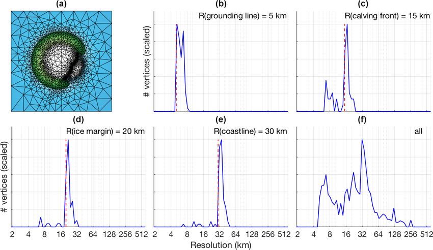
pendix E. Shown in Fig. 1 are four meshes generated for both acceleration g, ice thickness H , surface gradient ∇h, Glen’s
Antarctica and Greenland, based on present-day ice-sheet ge- flow law exponent n, and the temperature-dependent ice flow
ometry (BedMachine Greenland version 3, Morlighem et al., factor A(T ∗ ). For a comprehensive derivation of Eqs. (1)
2017, and BedMachine Antarctica version 1, Morlighem et and (2), see for example Bueler and Brown (2009). In or-
al., 2019), with maximum ice-margin (including both the der to calculate ice thickness changes over time, the depth-
grounding line and the calving front) resolutions of 100, dependent velocities in Eq. (2) are vertically averaged.
30, 10, and 3 km, respectively. For Antarctica, two high- A concrete version of the SSA stress balance, expressed
resolution locations are included: one at the South Pole, and in terms of the vertically averaged horizontal ice velocities
one at the EPICA Dome C drill site. u, v, is given by Bueler and Brown (2009). Here, subscripts
Since the ice margin, the calving front and the ground- ∂u
denote partial derivatives, e.g. ux = ∂x :
ing line are one-dimensional regions, increasing the desired
resolution only over these regions results in a total number ∂ ∂
of vertices and triangles that scales almost linearly with this 2νH 2ux + vy + νH uy + vx (3a)
∂x ∂y
resolution (though not quite, as increasing the resolution re- τc u
solves more geographical features, increasing the length of − = ρgH hx ,
|u|
the lines). How the number of vertices and the computational
∂ ∂
speed of the model scale with the prescribed resolution is in- νH uy + vx + 2νH ux + 2vy (3b)
vestigated in more detail in Sect. 4. UFEMISM uses a dy- ∂x ∂y
τc v
namic adaptive mesh, which is adapted to the modelled ice- − = ρgH hy .
sheet geometry during a simulation, so that the grounding |u|
line and other regions of interest are always captured at a The first two terms on the left describe the extensional
high resolution, even when the ice-sheet geometry changes stresses, also called “membrane stresses”. The third term de-
substantially. The exact way this is achieved is illustrated in scribes the basal shear stress for a Coulomb-type friction law,
Appendix E. which is commonly used in hybrid SIA–SSA models since
the vanishing friction at the grounding line yields better re-
sults than the discontinuous Weertman-type friction law. The
https://doi.org/10.5194/gmd-14-2443-2021 Geosci. Model Dev., 14, 2443–2470, 20212446 C. J. Berends et al.: The Utrecht Finite Volume Ice-Sheet Model: UFEMISM (version 1.0)
Figure 1. Meshes generated for Antarctica (a–d) and Greenland (e–h), based on present-day ice-sheet geometry, with maximum ice-margin
(including grounding line and calving front) resolutions of 100, 30, 10, and 3 km, respectively. For Antarctica, two high-resolution locations
are included: one at the South Pole, and one at the EPICA Dome C drill site. Both have been prescribed the same resolution as the ice margin.
right-hand side describes the gravitational driving stress. The servation of mass. The finite volume approach is explained
vertically averaged ice viscosity ν is described by MacAyeal in more detail in Appendix B.
(1989) as a function of ice velocity: The SIA and SSA are solved asynchronously, with the
time steps determined as a function of the local resolution
Zh Rc (defined as the distance between the two regular vertices
1 −1
ν= A T∗ n dz (4) connected by the staggered vertex vc ), the staggered SIA dif-
2 fusivity Dc , and the staggered SSA ice velocities uc , vc , sim-
b
1−n ilar to the approach used in PISM (Bueler et al., 2007):
1 2 2n
· u2x + vy2 + ux vy + uy + vx .
4 −Rc2
1tSIA = min , (6a)
c 6π Dc
In order to ensure proper grounding line migration, a semi-
analytical solution for grounding line flux with a Coulomb- Rc
1tSSA = min . (6b)
type sliding law (Tsai et al., 2015) is applied as a boundary c |uc | + |vc |
condition for the SSA:
2.4 Thermodynamics
8A(ρg)n ρi n−1 n+2
qg = Q0 n 1− Hg . (5) UFEMISM uses a mixed implicit–explicit finite differencing
4 tan ϕ ρw
scheme with a fixed time step to solve the heat equation in a
The way this solution is implemented is described in detail flowing medium:
in Appendix C.
∂T k 2 8
The way these equations are discretized on the unstruc- = ∇ T − u · ∇T + , (7)
tured triangular mesh is derived in Appendix A. Ice thickness ∂t ρcp ρcp
changes over time are then calculated using a finite volume ∂u ∂h ∂v ∂h
8 = 2 ε̇xz τxz + ε̇yz τyz = −ρg (h − z) + .
approach: by calculating both the surface slopes (∂h)/(∂x) ∂z ∂x ∂z ∂y
and (∂h)/(∂y) and the resulting ice velocities u and v, on (8)
the boundaries between vertices (using the “staggered mesh”
approach described in Appendix A), ice fluxes between indi- The three terms on the right-hand side of Eq. (7) respec-
vidual vertices are calculated explicitly, and moved from one tively represent diffusion, advection, and strain heating (us-
vertex to the other in every time step. This guarantees con- ing a strain heating expression that is valid only for the SIA;
Geosci. Model Dev., 14, 2443–2470, 2021 https://doi.org/10.5194/gmd-14-2443-2021C. J. Berends et al.: The Utrecht Finite Volume Ice-Sheet Model: UFEMISM (version 1.0) 2447
a simplification that will need to be addressed in future im- We performed several simulations with UFEMISM of an
provements). In UFEMISM, horizontal diffusion of heat is ice sheet that starts at t = t0 with the Halfar solution for H0 =
neglected, simplifying Eq. (7) to 5000 m, R0 = 300 km, A = 10−16 Pa3 yr−1 , and n = 3. The
ice-margin resolutions for the different simulations were set
∂T k ∂ 2T 8 to 50, 16, 8, and 4 km. Shown in Fig. 2 are transects of the
= 2
− u · ∇T + . (9)
∂t ρcp ∂z ρcp simulated ice sheet at different points in time, compared to
the analytical solution.
This equation is discretized on an irregular grid in the ver- UFEMISM reproduces the analytical solution well, with
tical direction; all vertical derivatives are discretized implic- the largest errors occurring at the margin, and decreasing
itly, whereas horizontal derivatives are discretized explicitly. with resolution. As was shown by Bueler et al. (2005), this is
This mixed approach has a long history of use in palaeo- the case for all spatially discrete SIA models and is due to the
ice-sheet models (e.g. Huybrechts, 1992; Greve, 1997), as fact that such models are intrinsically unable to reproduce the
it is numerically stable (since both the steepest gradients and infinite surface slope at the margin predicted by the contin-
shortest grid distances are in the vertical direction), relatively uum model. They also show that these errors do not “corrupt”
easy to implement, and fast to compute. Using 15 layers in the model solution over the interior. This matches our results,
the vertical direction, a time step of 10 years is typically suf- where the modelled ice-sheet interior after 100 000 years is
ficient to maintain numerical stability for the range of resolu- still close to the analytical solution. At that time, the mod-
tions investigated here. The iterative scheme for solving this elled ice-sheet margin at 4 km resolution differs from the an-
equation is derived in Appendix C. alytical solution by about 10 km.
A generalization of the solution by Halfar (1981), applica-
3 Model verification and benchmark experiments ble to problems including a simple elevation-dependent ac-
cumulation rate, was derived by Bueler et al. (2005). For an
In order to verify the numerical solution to the ice dynami- accumulation given by
cal equations, we performed several benchmark experiments, λ
where we compare our model output to analytical solutions Mλ (r, t) = H (r, t) (12)
t
(Halfar, 1981; Bueler et al., 2005), and to results from the
EISMINT intercomparison exercise (Huybrechts et al., 1996) the solution for the ice thickness over time reads as follows:
for the SIA part of the solution, and finally for the complete " n
# n+1 2n+1
α −β n
hybrid SIA–SSA to the MISMIP experiments (Pattyn et al. t0 t r
2012). All of the experiments were performed using the dy- Hλ (r, t) = H0 1− , (13)
t t0 R0
namic adaptive mesh.
2 − (n + 1) λ 1 + (2n + 1) λ
α= ,β= ,
3.1 Verification using analytical solutions 5n + 3 5n + 3
(14)
β 2n + 1 n R0n+1
For several schematic, simplified ice-sheet configurations, 2A
t0 = 2n+1
, 0= (ρg)n .
analytical solutions exist for the time evolution of the ice 0 n+1 H0 5
sheet. One of these was derived by Halfar (1981), describ-
The special case of zero mass balance, described by λ = 0,
ing a “similarity solution” for the time evolution of a radially
gives the solution by Halfar (1981). The results of this ex-
symmetrical, isothermal ice sheet lying on top of a flat bed,
periment are shown in Fig. 3, for the case of λ = 5, which
with a uniform zero mass balance. For an ice sheet which,
describes a positive accumulation rate, resulting in a rapidly
at time t0 , has a thickness at the dome H0 and margin radius
expanding ice sheet. Here, too, UFEMISM reproduces the
R0 , the time-dependent solution to the SIA, with Glen’s flow
analytical solution well, with the largest errors occurring at
law exponent n, reads as follows:
the ice-sheet margin and decreasing with resolution.
n
2 1 ! n+1
n
2n+1
3.2 EISMINT benchmark experiments
t0 5n+3 t0 5n+3 r
H (r, t) = H0 1 − ,
t t R
In order to further investigate the validity of our numeri-
cal schemes for ice dynamics and thermodynamics, we used
(10)
UFEMISM to perform the first set of EISMINT benchmark
R0n+1
n
1 2n + 1 2A experiments (Huybrechts et al., 1996). All of the six experi-
t0 = , 0= (ρg)n . (11)
(5n + 3) 0 n + 1 H02n+1 5 ments consist of a radially symmetric ice sheet, lying atop a
flat, non-deformable bedrock. While the temperature of the
Since the surface mass balance is zero, any change in ice ice is calculated dynamically, the ice flow factor is kept fixed
thickness is caused only by ice dynamics, making this a use- at a value of A = 10−16 Pa3 yr−1 , meaning that ice tempera-
ful experiment for verifying ice-sheet model numerics. ture is a purely diagnostic variable. The six experiments are
https://doi.org/10.5194/gmd-14-2443-2021 Geosci. Model Dev., 14, 2443–2470, 20212448 C. J. Berends et al.: The Utrecht Finite Volume Ice-Sheet Model: UFEMISM (version 1.0) Figure 2. The evolution through time of a schematic, radially symmetric, isothermal ice sheet, as simulated by UFEMISM at different ice-margin resolutions, compared to the Halfar solution starting at t = t0 . The small sub-panels in the top-right corner of the panels show a zoomed-in view of the ice margin, showing how the simulated ice margin converges to the analytical solution as the model resolution increases. Figure 3. The evolution through time of a schematic, radially symmetric, isothermal ice sheet, with positive accumulation rate, as simulated by UFEMISM at different ice-margin resolutions, compared to the Bueler (2005) solution. divided into two groups of three: a “moving margin” and a experiment were performed with ice-margin resolutions of “fixed margin” group (Table 1). In the “fixed margin” exper- the original EISMINT resolution of 50 km, as well as finer iments, the mass balance is such that the expected theoretical resolutions of 16, 8, and 4 km. ice margin lies outside the model domain, and ice thickness Shown in Fig. 4 are the simulated ice thickness and ice at the boundary is artificially kept at zero. In realistic model velocity of a radial transect of the ice sheet in experiment I, configurations, such a margin (i.e. where the ice thickness at the end of a 120 kyr simulation that was initialized with an does not approach zero) can occur at a calving front. A mov- ice thickness of zero. These results agree well with those pre- ing margin is achieved by setting a zero mass balance inte- sented by Huybrechts et al. (1996), showing an ice sheet that gral over a bounded region fully enclosed within the model is ∼ 2960 m thick at the divide and has a maximum outward domain. The three experiments within a group have differ- ice velocity of ∼ 55 m yr−1 at approximately 450 km away ent mass balances; a fixed, “steady-state” mass balance, one from the divide. The small sub-panel in the upper right cor- with an added 20 kyr sinusoid, and one with a 40 kyr sinu- ner of panel (a) zooms in on the ice margin, showing that the soid, which is useful for investigating the performance of the modelled ice margin converges to the analytical ice margin model in terms of temporal evolution. Simulations for each Geosci. Model Dev., 14, 2443–2470, 2021 https://doi.org/10.5194/gmd-14-2443-2021
C. J. Berends et al.: The Utrecht Finite Volume Ice-Sheet Model: UFEMISM (version 1.0)                                        2449

Table 1. The six different EISMINT experiments.                   Table 2. The step-wise flow factor changes in the MISMIP experi-
                                                                  ment.
             Experiment    Margin    Mass balance
                                                                            Time window      Flow factor (Pa−3 yr−1 )
             I             moving      steady-state
             II            moving           20 kyr                          0–25 kyr                  10−16
             III           moving           40 kyr                          25–50 kyr                 10−17
             IV             fixed      steady-state                         50–75 kyr                 10−16
             V              fixed           20 kyr
             VI             fixed           40 kyr

                                                                  3.3   MISMIP benchmark experiment

                                                                  In order to validate our solution to the hybrid SIA–SSA
(the perimeter of the circle where the mass balance integrates    stress balance, we performed the first MISMIP experiment
to zero) as the resolution increases.                             (Pattyn et al., 2012), modified from a 1-D flow line exper-
   Shown in Fig. 5 are the same transects for experiment          iment to 2-D plan-view experiment in a manner similar to
IV (steady-state, fixed margin), showing an ice sheet that is     Pattyn (2017). This schematic experiment consists of a cone-
∼ 3400 m thick at the divide, compared to 3340–3420 m in          shaped island at thep centre of the model grid (described by
Huybrechts et al. (1996).                                         b = 720 − 778.5 · x 2 + y 2 /(750 km)), under a spatially and
   Figures 6 and 7 show the temperature transect of the ice       temporally uniform mass balance forcing of 30 cm yr−1 . This
sheet for experiments I and IV at 4 km resolution, and the        results in a circular ice sheet, surrounded by an ice shelf that
basal temperature transects for all simulations in these exper-   extends to the domain boundary. In order to assess grounding
iments. Following the specifications from Huybrechts at al.       line dynamics in the model, the ice flow factor A is step-wise
(1996), the thermal conductivity and specific heat capacity of    increased (leading to grounding-line advance) and subse-
ice are kept fixed at uniform values of k = 2.1 J s−1 m−1 K−1     quently decreased (leading to grounding-line retreat). Pattyn
and cp = 2009 J kg−1 K−1 , respectively. Here, too, results       et al. (2012) showed that, while most participating ice-sheet
agree well with those reported by Huybrechts et al. (1996).       models produce some amount of grounding line advance in
In experiment I, basal temperatures at the ice divide are 11–     the first phase, many of them failed to retreat back to their ini-
12 K below the pressure melting point (PMP), increasing           tial position in the second phase. The “best” performance (i.e.
along the outward transect until they reach the PMP at 350–       a one-to-one relation between flow factor and grounding-line
400 km from the divide. In experiment IV we see similar re-       position, without any hysteresis) was observed in models that
sults, with basal temperatures at the ice divide lying around     included a semi-analytical solution to the grounding line flux
8 K below PMP, reaching PMP slightly further towards the          (Schoof, 2007; Tsai et al., 2015), either as a boundary con-
margin at 400–450 km from the divide. Preliminary exper-          dition to the SSA, or by overwriting the numerically derived
iments with a one-dimension set-up (vertical column only)         grounding line flux (typically using a heuristic rule to deter-
show that these results are robust across different choices of    mine which grid cells to apply the analytical solution to). We
vertical resolutions.                                             chose the former approach in UFEMISM, using the semi-
   Figure 8 shows the ice thickness change at the ice di-         analytical solution by Tsai et al. (2015) for a grounding line
vide over time for experiments II, III, V, and VI. Here too,      flux with a Coulomb-type sliding law, as a boundary condi-
the results from simulations with UFEMISM at different            tion in the SSA. This was achieved by solving the SSA simul-
resolutions agree with the results published by Huybrechts        taneously on both the regular and the “staggered” mesh (ex-
et al. (1996). The glacial–interglacial ice thickness (G–IG)      plained in more detail in Appendix C), and keeping the val-
changes for all four experiments lie within the ranges re-        ues on the staggered grounding line vertices (lying halfway
ported by Huybrechts et al. (1996), as listed in the top-right    between a grounded and a floating vertex) fixed at the analyt-
corners of both panels of Fig. 8. The simulated ice thickness     ical solution. We then prescribe a flow factor with step-wise
time series at different resolutions are not distinguishable.     changes every 25 000 years, as shown in Table 2. This exper-
Figure 9 shows the basal temperature relative to the pressure     iment was performed with grounding-line resolutions of 64,
melting point over time, for the same experiments. We find        32, and 16 km.
a G–IG temperature changes that are slightly smaller than            The results of this experiment with UFEMISM are shown
the values reported by Huybrechts et al. (1996), lying just       in Fig. 10. Panel (a) shows cross sections of the modelled
outside their reported ranges. In agreement with the findings     ice sheets at the end of the three time windows. As can be
of Huybrechts et al. (1996), introducing glacial cycles in the    seen, the ice sheets at 25 and 75 kyr are nearly indistinguish-
moving margin experiments (Fig. 9a) results in G–IG mean          able (as they should be for the same flow factor) and show no
temperature decrease of about 1 K, while the fixed margin ex-     appreciable dependence on resolution. Panel (b) shows the
periments (Fig. 9b) see a temperature increase of about 2.5 K.    grounding line position over time, showing that the ground-

https://doi.org/10.5194/gmd-14-2443-2021                                             Geosci. Model Dev., 14, 2443–2470, 2021
2450 C. J. Berends et al.: The Utrecht Finite Volume Ice-Sheet Model: UFEMISM (version 1.0)
Figure 4. (a) Ice thickness and (b) vertically averaged ice velocity of a radial transect of the ice sheet in experiment I, simulated by UFEMISM
at 50, 16, 8, and 4 km ice-margin resolutions. The vertical dashed line in (a) denotes the analytical ice margin.
Figure 5. (a) Ice thickness and (b) vertically averaged ice velocity of a radial transect of the ice sheet in experiment IV, simulated by
UFEMISM at 50, 16, 8, and 4 km ice-margin resolutions. The sharp peaks in the velocity near the margin are a result of the singularity in
these Nye–Vialov margins, and the ice thickness approaches zero as one approaches the margin, but the ice flux remains finite, implying an
infinite velocity.
ing line retreats exactly to its initial position after the flow 10 000 years. For these simulations, the climate was set to
factor is returned to its initial value, and that the results are the present-day observed climate (ERA-40; Uppala et al.,
resolution-independent. 2005) plus a spatially and temporally uniform 5 ◦ C warm-
ing. The version of UFEMISM presented here already in-
cludes the IMAU-ITM mass balance model (Fettweis et al.,
4 Computational performance 2020), so that a 5 ◦ C warming leads to a substantial retreat
through the increase in surface melt. The model was ini-
The first version of UFEMISM presented here is paral- tialized with the BedMachine Antarctica v2 (Morlighem et
lelized using the Message Passing Interface (MPI) construct al., 2019) bed topography and ice geometry. Sub-shelf melt
of “shared memory”, allowing the program to run in parallel was calculated using the temperature- or depth-dependent
on a number of processor cores that are able to directly ac- parameterization by Winkelmann et al. (2011) and Martin et
cess the same physical memory (usually either 16, 24, or 32 al. (2011), using a constant uniform ocean temperature. The
cores on typical computer clusters or supercomputers). This ice flow factor, thermal conductivity, specific heat, and pres-
is a temporary choice; the effort to extend the parallelization sure melting point were all calculated using the temperature-
to multiple nodes, using the full capability of MPI, is still dependent expressions given by Huybrechts (1992). The
ongoing but is beyond the scope of this paper. basal shear stress in the Coulomb-type sliding law imple-
In order to investigate the computational performance of mented in the SSA was calculated using the parameteriza-
the different model components, we performed a series of tions for the till friction angle and pore water pressure from
simulations of Antarctic ice-sheet retreat over a period of
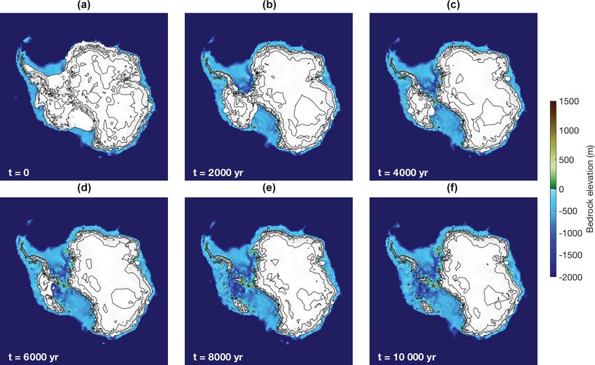
Geosci. Model Dev., 14, 2443–2470, 2021 https://doi.org/10.5194/gmd-14-2443-2021C. J. Berends et al.: The Utrecht Finite Volume Ice-Sheet Model: UFEMISM (version 1.0) 2451 Figure 6. (a) Ice temperature and velocity vectors for the steady-state ice sheet in experiment I, as produced by UFEMISM with a 4 km ice-margin resolution. (b) Basal temperature transects for the different simulations in the same experiment. Figure 7. (a) Ice temperature and velocity vectors for the steady-state ice sheet in experiment IV, as produced by UFEMISM with a 4 km ice-margin resolution. (b) Basal temperature transects for the different simulations in the same experiment. Martin et al. (2011). A constant, uniform geothermal heat ranging from bC = 0.71 for the SSA to bC = 0.83 for the flux of 1.72 × 10⁶ J m−2 yr−1 (Sclater et al., 1980) was pre- SIA. Mesh updating scales less well, with bC = 0.47. This is scribed. No glacial isostatic adjustment or changes in sea likely to do with the fact that the entire mesh generation code level were included. This experiment is not meant to rep- was writing by the authors themselves, instead of relying resent a realistic projection of Antarctic retreat; the choice upon available external software packages. Since mesh up- of forcing is merely convenient because it ensures a rapidly dating accounts for only 2 %–4 % of total computation time, changing ice-sheet geometry, forcing frequent mesh updates. this does not noticeably affect the parallelization of the com- The results of one of these simulations are shown in Fig. 11. plete model, which has bC = 0.74. The SSA dominates the The computation times of the different model components total computation time across all resolutions and numbers of as a function of number of cores and model resolution are processors, requiring as much or more computation time as shown in Fig. 12. The simulations described in Sect. 4 were all other model components combined. The routine that ap- run on the LISA computer cluster operated by SURFsara, plies the finite volume method described in Appendix B to using an Intel Xeon Gold 6130 Processor with a 2.1 GHz update the ice thickness through time is included in the SIA clock frequency and 22 MB cache, and were compiled with computation time. the ifort compiler. Figure 12b shows computation versus model resolution for Figure 12a shows the degree of parallelization of the the same model components. For each model component, model components. For each model component, logarithmic logarithmic fits have been made between the computation fits have been made between the computation time t and time t and the resolution R of the form ln t = a + bR ln R. In the number of cores C of the form ln t = a + bC ln C. The an idealized situation (such as the EISMINT experiments), coefficient bC describes the degree of parallelization, such the SIA and SSA should scale with the resolution to order that bC = 1 describes perfect parallelization, i.e. doubling the bR = 3 in a square-grid model (two orders from the number number of cores reduces the computation time by half. The of grid cells, and one from the time-step dependence on res- three physics modules have a good degree of parallelization, olution, according to the numerical stability criterion for the https://doi.org/10.5194/gmd-14-2443-2021 Geosci. Model Dev., 14, 2443–2470, 2021
2452                              C. J. Berends et al.: The Utrecht Finite Volume Ice-Sheet Model: UFEMISM (version 1.0)

Figure 8. (a) Ice thickness change at the divide for experiments II and III (moving margin, respectively 20 (blue) and 40 kyr (red) sinusoid
mass balance perturbation). (b) The same for the fixed margin experiments (V and VI), simulated by UFEMISM at 50, 16, 8, and 4 km ice-
margin resolutions. Listed in the top-right corners of both panels are the glacial–interglacial ice thickness changes simulated by UFEMISM,
compared to the ranges reported by Huybrechts et al. (1996) between brackets.

Figure 9. (a) Basal temperature change at the divide for experiments II and III (fixed margin, respectively 20 (blue) and 40 kyr (red) sinusoid
mass balance perturbation). (b) The same for the fixed margin experiments (V and VI), simulated by UFEMISM at 50, 16, 8, and 4 km
ice-margin resolutions. Listed in the top-right corners of both panels are the glacial–interglacial basal temperature changes simulated by
UFEMISM, compared to the ranges reported by Huybrechts et al. (1996) between brackets.

solution of the mass conservation equation). In UFEMISM,                  tion time. Preliminary experiments with a simple square-grid
this can be theoretically reduced to order bR = 2, since a high           model showed the same effect, and the computation time for
resolution is only applied over the one-dimensional ice-sheet             those experiments scaled with resolution to order bR = 3.5–
margin, where the diffusivity is not necessarily the largest              4.0, rather than the bR = 3 in the idealized case.
of the model domain. The reason that the results shown in                    The computation time of the mesh updating component
Fig. 12 deviate from this idealized case is because, for a re-            also scales well with model resolution, to the order bR =
alistic ice sheet, increasing the resolution resolves more to-            2.59. The thermodynamics component scales even better,
pographical features, which increases the length of the one-              with order bR = 0.95. The reason that this is so much lower
dimensional domains of the ice margin, the grounding line,                than the SIA and SSA components is that the thermodynam-
and the calving front. This is illustrated in Fig. 13, which              ics uses a constant rather than a dynamic time step, which is
shows the number of vertices of meshes for Greenland and                  related to the choice of vertical discretization rather than to
Antarctica versus the model resolution at the ice margin.                 the horizontal model resolution.
   Similarly, resolving more topographical features also leads               In these experiments, the entire ice margin, including the
to an increased ice diffusivity in areas with steep gradients,            grounding line and calving front, was given the same resolu-
decreasing the critical time step and increasing the computa-             tion. When using UFEMISM for actual palaeo-simulations,

Geosci. Model Dev., 14, 2443–2470, 2021                                                     https://doi.org/10.5194/gmd-14-2443-2021
C. J. Berends et al.: The Utrecht Finite Volume Ice-Sheet Model: UFEMISM (version 1.0)                                                   2453

Figure 10. (a) Cross sections of the modelled ice sheet at different times and different resolutions. (b) Grounding-line position over time for
the different resolutions.

Figure 11. Results from the 10 000-year Antarctic retreat simulation with a 4 km grounding line resolution. Panels (a–f) show the modelled
ice sheet at 2000-year intervals. Bedrock elevation is indicated by colours, surface elevation contours are shown at 1000 m intervals.

such a high resolution would only be used for the ground-                 they are at their maximum extent, while the Eurasian and
ing line, where it directly increases the physical accuracy of            Greenland ice sheets respectively require about one-half and
the solution. In one last experiment, we performed the same               one-quarter as much computation time. Based on these num-
Antarctic retreat simulation, with the resolution set to 4 km             bers, a full glacial cycle simulation of all four ice sheets
for the grounding line, 16 km for the rest of the ice mar-                would take somewhere between 1.5 and 3 times as much
gin, and 200 km over the ice sheet interior. Run on 16 cores,             as one for only Antarctica, implying a required computation
the simulation took about 88 core hours (5 h 30 m wall-clock              time of about 1600–3200 core hours (100–200 wall clock
time) to complete. Extrapolating these numbers to the Green-              hours on a 16-core system). For comparison, a full glacial cy-
land, North American, and Eurasian ice sheets is difficult,               cle simulation with ANICE at 40 km resolution takes about
due to the differences in size, glacial–interglacial geometry             8 core hours, which implies a simulation at 4 km would take
changes, and relative area of floating ice. Previous work with            about 25 000–80 000 core hours (numbers based on extrapo-
the square-grid model ANICE (Berends et al., 2018, 2019)                  lation), meaning that UFEMISM is about 10–30 times faster.
indicates that the Antarctic and North American ice sheets                If the grounding line resolution is decreased to 8 km, these
typically have roughly the same computational expense when                numbers decrease to about 200–600 core hours (20–40 wall

https://doi.org/10.5194/gmd-14-2443-2021                                                      Geosci. Model Dev., 14, 2443–2470, 2021
2454                                   C. J. Berends et al.: The Utrecht Finite Volume Ice-Sheet Model: UFEMISM (version 1.0)

Figure 12. (a) Computation times vs. number of cores for the SSA (blue), SIA (red), thermodynamics (yellow), and mesh updating (purple)
model components, as well as for the entire model (black), for a 10 000-year Antarctic retreat simulation at 8 km resolution. These four
components together account for ∼ 99.8 % of the total computation time. Logarithmic fits of the form ln t = a + bC ln C have been made to
the data, with the scaling coefficients bC shown in the legend. (b) Computation times vs. model resolution for the same model components,
run on 16 cores. Logarithmic fits of the form ln t = a + bR ln R have been made to the data, with the scaling coefficients bC shown in the
legend.

                                                                        cessors that can access the same shared memory chip. This
                                                                        means that it should be possible to compile and run the
                                                                        model on most consumer-grade systems. The model con-
                                                                        tains roughly 200 double precision data fields. For the 3 km
                                                                        resolution Antarctica mesh (∼ 100 000 vertices) shown in
                                                                        Fig. 1, this implies a memory usage of about 1.6 GB. Out-
                                                                        put is written to NetCDF files at about 10 kb per vertex,
                                                                        implying that a 120 kyr glacial cycle simulation of Antarc-
                                                                        tica at 3 km (100 000 vertices), where output is written every
                                                                        1000 model years, would generate about 150 GB of data.

                                                                        5   Conclusions and discussion

Figure 13. Number of vertices vs. ice-margin resolution for Green-      We have presented and evaluated a new thermomechani-
land and Antarctica.                                                    cally coupled ice-sheet model, UFEMISM, which solves the
                                                                        SIA and SSA versions of the ice-dynamical equations on a
Table 3. Observed and extrapolated computation times (in core           fully adaptive mesh. The model is able to accurately repro-
hours) for different simulations with ANICE and UFEMISM. Bold-          duce the analytical solutions for the evolution of schematic
faced numbers are observed times, all others are estimates based on     ice sheets by Halfar (1981) and Bueler et al. (2005), as
extrapolation.                                                          well as the EISMINT benchmark experiments (Huybrechts
                                                                        et al., 1996), indicating that the numerical schemes for solv-
  Experiment                                     ANICE     UFEMISM      ing the SIA and integrating the mass conservation law are
  10 kyr Antarctic retreat, 4 km               700–4500            88   valid. In a modified version of the first MISMIP experiment
  120 kyr glacial cycle (all ice), 40 km               8     2.5–12.5   (Pattyn et al., 2012), adapted from a 1-D flowline to a 2-D
  120 kyr glacial cycle (all ice), 8 km       2200–5000      200–600    plan view, UFEMISM shows a grounding line position that
  120 kyr glacial cycle (all ice), 4 km    25 000–80 000   1600–3200    is resolution-independent and displays no hysteresis during
                                                                        forced advance–retreat cycles. Analysis of the computational
                                                                        performance of the model indicates that it scales well with
hours) for UFEMISM, and 2200–5000 core hours for AN-                    both number of processors and model resolution. Based on
ICE. These numbers are summarized in Table 3.                           those results, UFEMISM should be able to simulate the evo-
   UFEMISM can be compiled with both the Gfortran and                   lution of the four large continental ice sheets over an entire
ifort compilers, requiring only LAPACK, NetCDF, and MPI                 glacial cycle, with a grounding line resolution of 4 km, in
as external packages, and can run on any number of pro-                 1600–3200 core hours (100–200 wall hours on 16 proces-

Geosci. Model Dev., 14, 2443–2470, 2021                                                  https://doi.org/10.5194/gmd-14-2443-2021
C. J. Berends et al.: The Utrecht Finite Volume Ice-Sheet Model: UFEMISM (version 1.0) 2455 sors), which is very feasible on typical facilities for scientific reduce this, including a spatially variable relaxation param- computation. eter (see Appendix B) and/or a multigrid scheme. Efforts to The MISMIP experiment (Pattyn et al., 2012) used here develop these solutions into applications that are robust and to validate our solution to the SSA requires further consid- stable enough for the large-scale, long-term simulations for eration. Pattyn et al. (2012) showed that simply solving the which UFEMISM is intended are ongoing but are beyond the SSA without any special treatment of the grounding line re- scope of this study. sults in grounding line positions that are strongly resolution- As UFEMISM is intended to be used for palaeo- dependent and yield significant hysteresis during advance– simulations, it has been developed to be able to include an retreat cycles, unless model resolution is lower than ∼ 100 m elaborate climate forcing and mass balance forcing. Previous (a value that is not feasible in palaeoglaciological simula- work by our group has focused on developing a computa- tions). This problem is not particular to the SSA, as the same tionally efficient climate forcing that explicitly includes im- problems are observed in the full-Stokes model Elmer/ice, portant feedback processes in the ice–climate system, such where a ∼ 30 km hysteresis in grounding-line position is ob- as the altitude–temperature feedback, ice–albedo feedback, served at a model resolution of 200 m (Gagliardini et al., and orographic precipitation feedback (Berends et al., 2018). 2016). Different semi-analytical solutions for the ice flux While these solutions have not yet been implemented in across the grounding line in the absence of buttressing have UFEMISM, it has been designed with these solutions in been proposed (Schoof, 2007; Tsai et al., 2015), and Pattyn mind, so that implementing them should be straightforward. et al. (2012) showed that using these solutions as a bound- Future work will also focus on improving the thermodynam- ary condition decreases both the resolution dependence and ics (probably using an energy-conserving enthalpy-based ap- the hysteresis (which is confirmed by our own results pre- proach along the lines of Aschwanden et al., 2012), adding sented here). However, implementing these analytical solu- a basal hydrology model (Bueler and van Pelt, 2015), and tions in 3D numerical models has proven difficult (Pollard including recently developed parameterizations for cliff fail- and DeConto, 2012; Pattyn et al., 2013), and recent work ure and shelf hydrofracturing (Pollard et al., 2015). We have has demonstrated that these analytical solutions cannot (yet) also previously worked on developing a coupled ice-sheet– be feasibly altered to account for buttressing (Reese et al., sea-level model (de Boer et al., 2014). A key improvement 2018b), which is absent in the MISMIP experiment we per- in UFEMISM with respect to our previous ice-sheet model is formed, but which plays an important role at the majority of the improved treatment of grounding line dynamics, which Antarctic grounding lines (Reese et al., 2018b). Our model makes it important to accurately account for changes in the therefore meets the same performance standards as existing geoid and the resulting changes in water depth at the ground- models for grounding line dynamics but probably does not ing line. While UFEMISM has not yet been coupled to a sea- produce correct grounding line dynamics under all circum- level model, it has been designed with such a future coupling stances, as the role of buttressing remains a matter of de- in mind. bate. Just how large an effect this has on palaeo-ice-sheet dy- namics relative to the uncertainties arising from proxy data, palaeoclimate forcing, and other physical processes, is still unclear. The current version of UFEMISM has been parallelised using MPI shared memory, meaning the number of proces- sors that can run the model depends on the hardware system, limited by how many processors can access the same mem- ory chip. The three most computationally expensive model components (the SSA, SIA, and thermodynamics modules, respectively) are shown to scale well. Extending the paralleli- sation framework to allow the model to run on multiple nodes might therefore substantially reduce the wall clock time for large simulations. The current version of UFEMISM uses do- main decomposition to parallelize the mesh generation algo- rithm. This approach lends itself well to multi-node paralleli- sation, as each node can be assigned a region of the model domain. The iterative scheme used in solving the SSA is currently the most computationally demanding model component, re- quiring as much or more computation time as all the other model components combined. Preliminary experiments have identified several possible solutions that could substantially https://doi.org/10.5194/gmd-14-2443-2021 Geosci. Model Dev., 14, 2443–2470, 2021
2456 C. J. Berends et al.: The Utrecht Finite Volume Ice-Sheet Model: UFEMISM (version 1.0)
t 1 h (t+1)∗ t i (t+1)∗ t i
i
Appendix A: Discretizing derivatives on an Ny,tri = x − x , x − x , x − x . (A3b)
unstructured triangular mesh ntz
Equation (A2) can then be written as
A1 First-order partial derivatives ∗
t
fx,tri = f i Nx,tri
t
(1) + f t Nx,tri
t t
(2) + f (t+1) Nx,tri (3), (A4a)
In UFEMISM, derivatives are discretized on the unstruc- t ∗
fy,tri = f i Ny,tri
t
(1) + f t Ny,tri
t t
(2) + f (t+1) Ny,tri (3). (A4b)
tured triangular mesh using an averaged-gradient approach.
In short, gradients are defined on the triangles surrounding a We approximate the derivative fxi of f on vertex i by aver-
vertex (which are piecewise smooth surfaces, having unique aging the derivatives on the n surrounding triangles:
gradients). The gradient on a vertex is then defined simply
n
as the average of the gradients on the surrounding triangles. 1X
fxi = ft (A5)
In the following derivation, we will show that this results n t=1 x,tri
in a linear combination of the function values on a vertex n h
and its direct neighbours. These coefficients, which we here 1X ∗
i
= f i Nx,tri
t
(1) + f t Nx,tri
t t
(2) + f (t+1) Nx,tri (3)
call “neighbour functions” (also known as “numerical sten- n t=1
cils”), are a function of mesh geometry, which means they 1X n 1X n
= fi t
f t Nx,tri
t
need to be calculated only once for a new mesh, and can Nx,tri (1) + (2)
n t=1 n t=1
be stored in memory for later use. This averaged-gradient
approach is very similar to an unweighted least-squares ap- n h
1X ∗ t
i
proach (Syrakos et al., 2017), and in Sect. A3 we will show + f (t+1) Nx,tri (3) .
n t=1
that, as expected, the resulting accuracy is second-order con-
vergent for the first derivatives fx and fy , and first-order con- Lowering the indices in the last sum term by one, this can be
vergent for the second derivatives fxx , fxy , and fyy . rearranged to read as follows:
Before getting started, we introduce “star notation” as n
1X
shorthand for the modulo function: i ∗ = mod(in). Using this fxi = ft (A6)
notation, “the next neighbour vertex counter-clockwise from n t=1 x,tri
neighbour s” becomes (s + 1)∗ , while “the next surrounding 1X n 1X n
= fi t
f t Nx,tri
t
triangle clockwise from triangle t” becomes (t − 1)∗ . Nx,tri (1) + (2)
n t=1 n t=1
Consider the unstructured triangular mesh in Fig. A1. We
n h
first define the partial derivatives fx and fy of a function f on 1X (t−1)∗
i
the triangles surrounding vertex i. Since these triangles are + f t Nx,tri (3)
n t=1
plane sections, they have well-defined first-order derivatives, n
which can be expressed using the normal vector to the plane. 1X
= fi N t (1)
Treating the value f i of f on vertex i as a coordinate in a n t=1 x,tri
third dimension, we can define v i = x i , y i , f i , such that
n h
1X
(t−1)∗
i
the upward normal vector nt to triangle t, spanned by v i , v t , + f t Nx,tri
t
(2) + Nx,tri (3) .
∗ n t=1
and v (t+1) , is given by
∗
This can be simplified by introducing the neighbour func-
nt = v t − v i × v (t+1) − v i (A1) tions Nxi on vertex i:
∗ ∗ ∗ n
f i y (t+1) − y t + f t y i − y (t+1) + f (t+1) y t − y i 1X
Nxi = t
i t (t+1)∗
t
(t+1)∗ − x i + f (t+1)∗ x i − x t .
Nx,tri (1) (A7a)
=
f x − x + f x n t=1
∗ ∗
xt − xi y (t+1) − y i − y t − y i x (t+1) − x i 1 t (t−1)∗
Nxi,t = Nx,tri (2) + Nx,tri (3) . (A7b)
n
The first-order spatial derivatives t
fx,tri and t
fy,tri of f on t This simplifies Eq. (A6) to
are then given by
n
X
−nty fxi = f i Nxi + f t Nxi,t . (A8)
t −ntx t
fx,tri = f = . (A2) t=1
ntz y ntz
For vertices lying on the domain boundary, which therefore
These expressions can be simplified by introducing the have n neighbours but n − 1 surrounding triangles, it can be
“neighbour functions” on triangle t: shown that the neighbour functions can be expressed as
n−1
1 h i 1 X
∗ ∗
Nxi = t
t
Nx,tri = t y t − y (t+1) , y (t+1) − y i , y i − y t (A3a) n − 1 t=1
Nx,tri (1) , (A9a)
nz
Geosci. Model Dev., 14, 2443–2470, 2021 https://doi.org/10.5194/gmd-14-2443-2021C. J. Berends et al.: The Utrecht Finite Volume Ice-Sheet Model: UFEMISM (version 1.0) 2457
Figure A1. A very simple unstructured triangular mesh. The vertex Figure A2. The geometric centres of the triangles surrounding ver-
under consideration, v i , is surrounded by its neighbours v n1 to v n6 , tex v i make up the vertices of a new set of “sub-triangles”, which
which together span triangles t 1 to t 6 . All neighbouring vertices and can be used to define the second derivative of a function on vertex
triangles are ordered counter-clockwise. vi .
1 1 if t = 1, dinate) is then given by
n−1 Nx,tri (2)
1 n−1
Nxi,t = n−1 N x,tri (3) if t = n,
∗
(A9b) nsx = v sx − v ix × v (s+1) − v ix (A11)
∗ x
1 N t (2) + N (t−1) (3)
otherwise.
n−1 x,tri x,tri "
(s+1)∗
#
1 f y i
−y +f
x
(s+2)∗
2y − y s
−y s
+f
x,tri
i (s+1)∗ (s+2)∗
x,tri
∗
y s + y (s+1) − 2y i
= (s+1)∗
.
f x −x i+f s x (s+2)∗
+x s
− 2x + f (s+1)∗ (s+2)∗ i i s
2x − x − x (s+1)∗
x x,tri x,tri
3 x + x − 2x y + y − 2y − y + y
1
3
s (s+1)∗ i (s+1)∗ (s+2)∗ i 1
3
s (s+1)∗ − 2y i
∗ ∗
x (s+1) + x (s+2) − 2x i
A2 Second-order partial derivatives s
The second-order derivatives fxx,sub s
and fxy,sub of f on s
are then given by
In order to discretize the second derivatives fxx , fxy , and
fyy , we treat the geometric centres of the triangles surround- s −nsx,x
fxx,sub = , (A12a)
ing vertex i as “staggered” vertices, where the staggered first nsx,z
derivatives are calculated according to Eq. (A4). We then −nsx,y
construct a new set of “sub-triangles”, spanned by the ver- s
fxy,sub = s . (A12b)
tex i and these staggered vertices, as illustrated in Fig. A2. nx,z
Since we know the values of fx and fy on all of them, we We then introduce the “sub-triangle neighbour functions”,
can use the same approach as before to calculate the gradi- similar to Eqs. (A3) (which, again, depend only on mesh ge-
ents of the first derivatives (i.e. the second derivatives) on ometry):
the sub-triangles, and average them to get the values on ver-
tex i. Preliminary experiments showed that using the geo-
s 1 s ∗
∗ ∗
metric centre instead of the circumcentre yields more stable Nx,sub = s y − y (s+2) , y (s+1) + y (s+2) − 2y i ,
nx,z
solutions when using these to solve differential equations. A (A13a)
mathematical proof of why this is the case might be interest-
∗
ing but lies beyond the scope of this study. 2y i − y s − y (s+1) ,
A new, staggered vertex in triangle t is created, using the
horizontal coordinates of the geometric centre of t, and the 1
∗
∗ ∗
s
t
derivative fx,tri of f on t as the vertical coordinate: Ny,sub = x (s+2) − x s , 2x i − x (s+1) − x (s+2) ,
nsx,z
" ∗ ∗
# (A13b)
x i + x t + x (t+1) y i + y t + y (t+1)
v tx t
= , , fx,tri . (A10)
∗
3 3 x s + x (s+1) − 2x i .
(s+1)∗ Substituting these into Eqs. (A12) yields
The sub-triangle
i i i s is spanned by v ix , v sx , and v x , where
i i
v x = x , y , fx (with fx as given by Eq. A8). The normal s
fxx,sub = fxi Nx,sub
s s
(1) + fx,tri s
Nx,sub (2) (A14a)
vector nsx to sub-triangle s (using the derivatives of f on the
(s+1)∗ s
vertex i and the triangles s and (s + 1)∗ as the vertical coor- + fx,tri Nx,sub (3),
https://doi.org/10.5194/gmd-14-2443-2021 Geosci. Model Dev., 14, 2443–2470, 2021You can also read