FOCUS: Clustering Crowdsourced Videos by Line-of-Sight
←
→
Page content transcription
If your browser does not render page correctly, please read the page content below
FOCUS: Clustering Crowdsourced Videos by Line-of-Sight

                                                  Puneet Jain                             Justin Manweiler
                                                 Duke University                           IBM T. J. Watson
                                        puneet.jain@duke.edu                         jmanweiler@us.ibm.com

                                                Arup Acharya                                 Kirk Beaty
                                                IBM T. J. Watson                           IBM T. J. Watson
                                            arup@us.ibm.com                          kirkbeaty@us.ibm.com

ABSTRACT                                                                             1.   INTRODUCTION
Crowdsourced video often provides engaging and diverse                               With the ubiquity of modern smartphones, photo and video
perspectives not captured by professional videographers.                             journalism is no longer limited to professionals. By virtue
Broad appeal of user-uploaded video has been widely                                  of having a Internet-connected videocamera always at arms’
confirmed: freely distributed on YouTube, by subscription on                         reach, the average person is always ready to capture and
Vimeo, and to peers on Facebook/Google+. Unfortunately,                              share exciting or unexpected events. With the advent of
user-generated multimedia can be difficult to organize; these                        Google Glass, the effort required to record and share will
services depend on manual “tagging” or machine-mineable                              soon disappear altogether. The popularity of YouTube and
viewer comments. While manual indexing can be effective                              video sharing on social media (e.g., Facebook and Google+)
for popular, well-established videos, newer content may be                           is evidence enough that many already enjoy creating and
poorly searchable; live video need not apply. We envisage                            distributing their own video content, and that such video
video-sharing services for live user video streams, indexed                          content is valued by peers. Indeed, major news organizations
automatically and in realtime, especially by shared content.                         have also embraced so-called “citizen journalism,” such as
We propose FOCUS, for Hadoop-on-cloud video-analytics.                               CNN iReport, mixing amateur-sourced content with that of
FOCUS uniquely leverages visual, 3D model reconstruction                             professionals, and TV broadcasting this content worldwide.
and multimodal sensing to decipher and continuously
track a video’s line-of-sight. Through spatial reasoning on                          Amateur video need not be immediately newsworthy to be
the relative geometry of multiple video streams, FOCUS                               popular or valuable. Consider a sporting event in a crowded
recognizes shared content even when viewed from diverse                              stadium. Often, spectators will film on their smartphones,
angles and distances. In a 70-volunteer user study, FOCUS’                           later posting these videos to YouTube, Facebook, etc. Even
clustering correctness is roughly comparable to humans.                              if their content is generally mundane, these videos capture
                                                                                     the unique perspective of the observer, and views potentially
                                                                                     missed by professional videographers, even if present. Unfor-
Categories and Subject Descriptors                                                   tunately, given a multitude of sources, such video content is
H.3.4 [Information Storage and Retrieval]: Systems and                               difficult to browse and search. Despite the attempts of sev-
Software                                                                             eral innovative startups, the value can be lost due to a “nee-
                                                                                     dle in a haystack” effect [3–6]. To organize, websites like
General Terms                                                                        YouTube rely on an haphazard index of user-provided tags
                                                                                     and comments. While useful, tags and comments require
Algorithms, Design, Experimentation, Performance                                     manual effort, may not be descriptive enough, are subject to
                                                                                     human error, and may not be provided in realtime — thus,
Keywords                                                                             not amenable to live video streams. In contrast, we envis-
Crowdsourcing, Line-of-sight, Live Video, Multi-view Stereo                          age a realtime system to extract content-specific metadata for
                                                                                     live video. Unlike related work applying lightweight sensing
                                                                                     in isolation [1], our approach blends sensing with computer
                                                                                     vision. This metadata is sufficiently precise to immediately
                                                                                     identify and form “clusters” of synchronized streams with re-
                                                                                     lated content, especially, a precise subject in shared “focus.”

                                                                                     In this paper, we propose FOCUS, a system for realtime anal-
Permission to make digital or hard copies of all or part of this work for
personal or classroom use is granted without fee provided that copies are            ysis and clustering of user-uploaded video streams, especially
not made or distributed for profit or commercial advantage and that copies           when captured in nearby physical locations (e.g., in the same
bear this notice and the full citation on the first page. To copy otherwise, to      stadium, plaza, shopping mall, or theater). Importantly, FO-
republish, to post on servers or to redistribute to lists, requires prior specific   CUS is able to deduce content similarity even when videos are
permission and/or a fee.                                                             taken from dramatically different perspectives. For example,
SenSys ’13, November 11 - 15 2013, Roma, Italy
                                                                                     two spectators in a soccer stadium may film a goal from the
Copyright 2013 ACM 978-1-4503-2027-6/13/11 ...$15.00.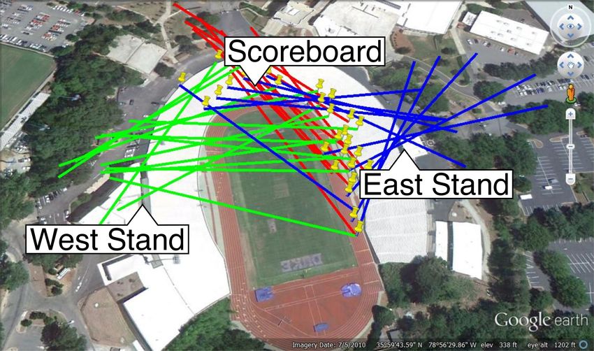
East and West stands, respectively. With up to 180 degrees           is community-sourced video on Facebook and Google+. The
of angular separation in their views, each spectator may cap-        value of particular shared content, however, can be lost in
ture a distinct (uncorrelated) background. Even the shared           volume, due to the difficulty of indexing multimedia. Today,
foreground subject, the goalkeeper, will appear substantially        user-generated “tags” or mineable text comments aid peers
different when observed over her left or right shoulder. With-       while browsing rich content. Unfortunately, newer and
out a human understanding of the game, it would be diffi-            real-time content cannot benefit from this metadata.
cult to correlate the East and West views of the goalkeeper,
while distinguishing from other players on the field. Novelly,       We envisage large-scale sharing of live user video from smart-
FOCUS’ analysis reasons about the relative camera location           phones. Various factors are enabling: the pervasiveness of
and orientation of two or more video streams. The geomet-            smartphones and increasing use of social apps; improving cel-
ric intersection of line-of-sight from multiple camera views is      lular data speeds (e.g., 4G LTE); ubiquity of Wi-Fi deploy-
indicative of shared content. Thus, FOCUS is able to infer log-      ments; increased availability and adoption of scalable, cloud-
ical content similarity even when video streams contain little       based computation, useful for low-cost video processing and
or no visual similarity.                                             distribution; enhanced battery capacity, computational capa-
                                                                     bilities, sensing, and video quality of smartphones; and the
Users record and upload video using our Android app,                 advent of wearable, wirelessly-linked videocameras for smart-
which pairs the video content with precise GPS-derived               phones, such as in Google Glass.
timestamps and contextual data from sensors, including GPS,
compass, accelerometer, and gyroscope. Each video stream             The dissemination of live, mobile, crowdsourced multimedia
arrives at a scalable service, designed for deployment on            is relevant in a variety of scenarios (e.g., sports). However,
an infrastructure-as-a-service cloud, where a Hadoop-based           to extract this value, its presentation must not be haphazard.
pipeline performs a multi-sensory analysis. This analysis            It must be reasonably straightforward to find live streams of
blends smartphone sensory inputs along with structure from           interest, even at scales of hundreds or thousands of simultane-
motion, a state-of-the-art technique from computer vision.           ous video streams. In this paper, we propose FOCUS, a system
For each stream, FOCUS develops a model of the user’s                to enable an organized presentation, especially designed for
line-of-sight across time, understanding the geometry of the         live user-uploaded video. FOCUS automatically extracts con-
camera’s view — position and orientation, or pose. Across            textual metadata, especially relating to the line-of-sight and
multiple user streams, FOCUS considers video pairs, frame            subject in “focus,” captured by a video feed. While this meta-
by frame. For each pair, for each frame, FOCUS determines            data can be used in various ways, our primary interest is to
commonality in their respective lines-of-sight, and assigns          classify or cluster streams according to similarity, a notion of
a “similarity” score. Across multiple feeds, across multiple         shared content. In this section, we will consider what it means
frames, these scores feed a pairwise spatiotemporal matrix           for a pair of video streams to be judged as “similar,” consider
of content similarity. FOCUS applies a form of clustering on         approaches and metrics for quantifying this understanding of
this matrix, invoking ideas from community identification in         similarity, and identify challenges and opportunities for ex-
complex networks, returning groups with a shared subject.            tracting metric data on commodity smartphones.

FOCUS remains an active research project, as we endeavor to          2.1    Characterizing Video Content Similarity
further harden its accuracy and responsiveness. However, de-         While there can be several understandings of “video similar-
spite ample room for further research, we believe that FOCUS         ity,” we will consider two videos streams to be more similar
today makes the following substantial contributions:                 if, over a given period of time, a synchronized comparison of
     1. Novel Line-of-Sight Video Content Analysis: FOCUS            their constituent frames demonstrates greater “subject simi-
        uses models derived from multi-view stereo reconstruc-       larity.” We judge two frames (images) to be similar depend-
        tion to reason about the relative position and orientation   ing on how exactly each captures the same physical object.
        of two or more videos, inferring shared content, and pro-    Specifically, that object must be the subject, the focal intent of
        viding robustness against visual differences caused by       the videographer. By this definition, subject-similar clusters
        distance or large angular separations between views.         of live video streams can have several applications, depend-
                                                                     ing on the domain. In sporting events, multiple videos from
     2. Inertial Sensing for Realtime Tracking: Despite an           the same cluster could be used to capture disparate views of a
        optimized Hadoop-on-cloud architecture, the computa-         contentious referee call, allowing viewers to choose the most
        tional latency of visual analysis remains substantial. FO-   amenable angle of view — enabling a crowdsourced “instant
        CUS uses lightweight techniques based on smartphone          replay.” For physical security, multiple views of the same sub-
        sensors, as a form of dead reckoning, to provide contin-     ject can aid tracking of a suspicious person or lost child. For
        uous realtime video tracking at sub-second timescales.       journalism, multiple views can be compared, vetting the in-
     3. Clustering Efficacy Comparable to Humans: In a 70-           tegrity of an “iReport.”
        volunteer study, clustering by modularity maximization       It is important to note that this definition of similarity says
        on a “spatiotemporal” matrix of content similarity yields    nothing of the perspective of the video (i.e., the location from
        a grouping correctness comparable to humans, when mea-       where the video is captured), so long as the foreground sub-
        sured against the ground truth of videographer intent.       ject is the same. We believe our definition of similarity, where
                                                                     the angle of view is not considered significant, is especially
2.     INTUITION                                                     relevant in cases of a human subject. Naturally, two videos
User-generated, crowdsourced, multimedia has clear value.            of a particular athlete share “similar” content, regardless of
YouTube and other sharing sites are immensely popular, as            from which grandstand she is filmed. However, if these videos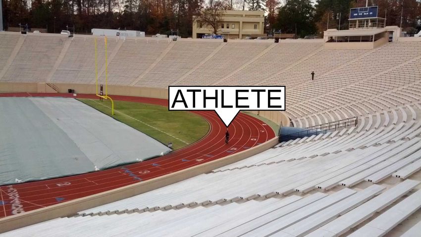
Field-of-View
Field-of-View
Line-of-Sight
Figure 2: Illustrating line-of-sight: (a) users film two soc-
cer players, ideally defining two clusters, one for each; (b)
line-of-sight can be better understood as a 3D pyramid-
shaped region, capturing the camera’s horizontal and ver-
tical field-of-view angles.
similarity of the corresponding videos, at the corresponding
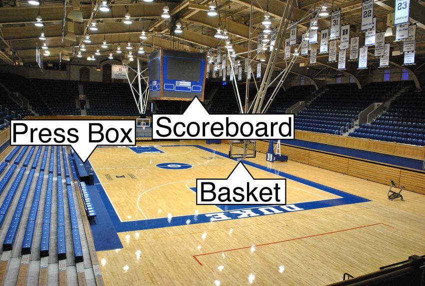
Figure 1: Time-synchronized frames from four videos of precise instant in time. A maximally-similar pair of views will
an athlete on a stadium running track. Note that these have line-of-sight rays that perfectly intersect in 3D — the
frames are considered “similar,” capturing the same ath- intersection point will be within the volume of their mutual
lete, but “look” heterogeneous. subject (e.g., person or building). Line-of-sight rays which do
not nearly intersect will not be similar. Figure 2 illustrates
are captured from a wide angular separation, they may “look”
that, with multiple videos, intersecting line-of-sight rays sug-
quite distinct. Contingent on the angle of separation, the vi-
gest shared video content. Consistency across time reinforces
sual structure and color of an object or person, lighting con-
the indication.
ditions (especially due to the position of the sun early or late
in the day), as well as the background, may vary considerably. Strictly, and as illustrated by the left athlete in Figure 2(a), in-
Perhaps counterintuitively, two “similar” views might actually tersecting line-of-sight rays does not guarantee a shared sub-
look quite different (Figure 1). Our techniques must accom- ject. The principle subject of each video may appear in the
modate this diversity of view. Using the techniques we de- foreground of (or behind) the intersection point. Thus, an
scribe in Section 3, it would also be possible to judge a pair inference of similarity by line-of-sight must be applied judi-
of videos shot from a more-nearby location as more similar. ciously. In Section 3, we explain how FOCUS’s similarity met-
However, we see fewer immediate applications of this defini- ric leverages vision to roughly estimate the termination point
tion, and henceforth exclude it. of a line-of-sight vector, substantially reducing the potential
for false positive similarity judgments.
By our definition, videos which look heterogeneous may be
judged similar, if they share the same subject. Further, videos Our system, FOCUS, leverages multi-view stereo reconstruc-
which look homogenous may be judged dissimilar, if their sub- tions and gyroscope-based dead-reckoning to construct 3D ge-
jects are physically different. For example, videos that capture ometric equations for videos’ lines-of-sight, in a shared co-
different buildings, but look homogenous due to repetitive ar- ordinate system. More precisely, we will define four planes
chitectural style, should not be considered similar. Thus, a per video frame to bound an infinite, pyramid-shaped vol-
system to judge similarity must demonstrate a high certainty ume of space, illustrated in Figure 2(b). The angular sepa-
in deciding whether the object in a video’s focus is truly the ration between these planes corresponds to the camera’s field-
same precise subject in some other video. of-view, horizontally and vertically, and is distributed symmet-
rically across the line-of-sight ray. Geometric and computer
Visual Metrics for Content Similarity. Understanding vision calculations, considering how thoroughly and consis-
that two videos that “look” quite different might be judged tently these pyramid-shaped volumes intersect the same phys-
“similar,” and vice versa, several otherwise-reasonable tech- ical space, will form the basis for a content similarity metric.
niques from vision are rendered less useful. Histograms of
color content, spatiograms [10], and feature matching [33], To simplify, FOCUS understands the geometric properties of
are valuable for tracking an object across frames of a video the content observed in a video frame, according to line-of-
though a “superficial” visual similarity. However, they are sight and field-of-view. FOCUS compares the geometric rela-
not intended to find similarity when comparing images tionship between the content one video observes with that of
that, fundamentally, may share little in common, visually. others. If a pair of videos have a strong geometric overlap, in-
Though complementary to our approach, visual comparison dicating that they both capture the same subject, their content
is insufficient for our notion of subject-based similarity. is judged to be “similar.” Ultimately, groups of videos, shar-
ing a common content, will be placed in self-similar groups,
Leveraging Line-of-Sight. Our definition of similarity re- called clusters. Clusters are found through a technique called
quires a precise identification of a shared subject (difficult). weighted modularity maximization, borrowed from community
One possible proxy is to recognize that a pair of videos cap- identification in complex networks. FOCUS finds “communi-
ture some subject at the same physical location. If we know that ties” of similar videos, derived from their geometric, or “spa-
a pair of videos are looking towards the same location, at the tial” relationship with time. Thus, uniquely, we say FOCUS
same time, this strongly indicates that they are observing the groups live user videos streams based on a spatiotemporal
same content. Precisely, we can consider the line-of-sight of metric of content similarity.
a video, geometrically, a vector from the camera to the sub-
ject. More practically, we can consider the collinear infinite 2.2 Opportunities to Estimate Line-of-Sight
ray from the same point-of-origin and in the same direction. With the availability of sensors on a modern smartphone, it
The geometric relationship of a pair of these rays reflects the may seem straightforward to estimate a video’s line-of-sight: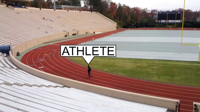
GPS gives the initial position; compass provides orientation.      name our system FOCUS (Fast Optical Clustering of User
Unfortunately, limited sensor quality and disruption from the      Streams). FOCUS leverages those visual inputs to precisely
environment (e.g., difficulty obtaining a high-precision GPS       estimate a video stream’s line-of-sight. Geometric and sen-
lock due to rain or cloud cover, presence of ferromagnetic         sory metadata provides context to inform a spatiotemporal
material for compass) may make line-of-sight inferences            clustering, derived from community identification, to find
too error-prone and unsuitable for video similarity analysis.      groups of subject-similar videos. The FOCUS design, while
Figure 3 illustrates this imprecision; lines of the same color     willing to exercise substantial computation, is considered
should converge. Further, GPS is only useful outdoors —            with a view towards real-world deployability, emphasizing
applications in indoor sporting arenas, shopping malls, and        (1) scalability, leveraging a cloud-based elastic architecture,
auditoriums would be excluded. Of course, a sensing-only           and (2) computational shortcuts, blending computer vision
approach can be valuable in some scenarios: outdoors when          with inertial sensing inputs into a hybrid analysis pipeline.
a reduced precision is tolerable. In Section 3.5, we use
GPS, compass, and gyroscope for a lightweight clustering,          Architectural Overview
formulated to minimize the impact of compass imprecision.          The FOCUS architecture includes: (1) a mobile app (proto-
                                                                   typed for Android) and (2) a distributed service, deployed
Smartphone sensing is, in general, insufficient for estimating     on an infrastructure-as-a-service cloud using Hadoop. The
a video’s line-of-sight. The content of video itself, however,     app lets users record and upload live video streams annotated
presents unique opportunities to extract detailed line-of-sight    with time-synchronized sensor data, from GPS, compass, ac-
context. Using the well-understood geometry of multiple views      celerometer, and gyroscope. The cloud service receives many
from computer vision, it is possible to estimate the perspec-      annotated streams, analyzing each, leveraging computer vi-
tive from which an image has been captured. In principle,          sion and sensing to continuously model and track the video’s
if some known reference content in the image is found, it is       line-of-sight. Across multiple streams, FOCUS reasons about
possible to compare the reference to how it appears in the         relative line-of-sight/field-of-view, assigns pairwise similarity
image, deducing the perspective at which the reference has         scores to inform clustering, and ultimately identifies groups of
been observed. At the most basic level, how large or small         video streams with a common subject.
the reference appears is suggestive of from how far away it
has been captured. In the next section, we describe how our        Figure 4 illustrates the overall flow of operations in the FO-
solution leverages structure from motion, a technique enabling     CUS architecture. We describe the key components in this
analysis and inference of visual perspective, to reconstruct the   section. We (1) describe computer vision and inertial sens-
geometry of a video line-of-sight.                                 ing techniques for extracting an image’s line-of-sight context;
                                                                   (2) consider metrics on that context for assigning a similar-
Both smartphone sensing and computer vision provide                ity score for a single pair of images; (3) present a clustering-
complimentary and orthogonal approaches for estimating             based technique to operate on a two-dimensional matrix of
video line-of-sight. This paper seeks to blend the best aspects    similarity scores, incorporating spatial and temporal similar-
of both, providing high accuracy and indoor operation (by          ity, to identify self-similar groups of videos; (4) explain how
leveraging computer vision), taking practical efforts to reduce    computations on the Hadoop-on-cloud FOCUS prototype have
computational burden (exploiting gyroscope), and providing         been optimized for realtime operation; and (5) describe a
failover when video-based analysis is undesirable (using           lightweight, reduced accuracy sensing-only technique for line-
GPS/compass/gyroscope). We actualize our design next,              of-sight estimation, for use in cases when computer vision
incorporating this hybrid of vision/multimodal sensing.            analysis is undesirable or impractical.

3.   ARCHITECTURE AND DESIGN                                       3.1    Line-of-Sight from Vision and Gyroscope
Fundamentally, an accurate analysis of content similarity          By leveraging an advanced technique from computer vision,
across video streams must consider the video content itself        Structure from Motion (SfM), it is possible to reconstruct a 3D
— it most directly captures the intent of the videographer.        representation, or model, of a physical space. The model con-
Accordingly, reflecting the importance of visual inputs, we        sists of many points, a point cloud, in 3D Euclidean space. It
                                                                   is possible to align an image (or video frame) to this model
                                                                   and deduce the image’s camera pose, the point-of-origin lo-
                                                                   cation and angular orientation of line-of-sight, relative to the
                                                                   model. Multiple alignments to the same model infer line-of-
                                                                   sight rays in a single coordinate space, enabling an analysis
                                                                   of their relative geometry. As noted in Figure 4, FOCUS lever-
                                                                   ages Bundler [37], an open source software package for SfM,
                                                                   both for the initial model construction and later video frame-
                                                                   to-model alignment.

                                                                   While the SfM technique is complex (though powerful and
                                                                   accurate), its usage is straightforward. Simply, one must take
                                                                   several photographs of a physical space (while a minimum of
Figure 3: Google Earth view of a stadium with impre-               four is sufficient, efficacy tends to improve with a much larger
cise line-of-sight estimates from GPS/compass: (green)             number of photos). With these images as input, SfM operates
towards West Stands, left; (red) towards Scoreboard, top;          in a pipeline: (1) extraction of the salient characteristics of
(blue) towards East Stands, right.                                 a single image, (2) comparison of these characteristics across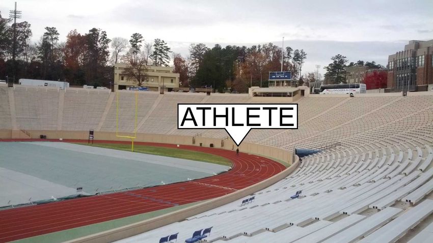
Sensing Data: Accelerometer,
Compass, GPS, Gyroscope Video written to Hadoop
Distributed File System (HDFS)
Video and Sensor Spatiotemporal Clustering Photographs
Video/Sensor Data in HDFS by Modularity Maximization
FOCUS
App Upload Service
Live Video Spatiotemporal Application One-time
Checkpointing Model
Similarity Matrix
Hadoop Processing Queues Generation
Stream Live! (multiple videos, tasks in flight) Bundler SfM Alignment
Video Download Service
SIFT Keypoint Extraction
(Example Application)
Video read from HDFS Extracted
Frames
(Example Application) Hadoop Mapper
Bundler
SfM 3D Model
Cloud Virtual Machines Hadoop Parallel Processing
Figure 4: Overall FOCUS architecture. Note that video frame extraction, feature analysis, and alignment to an SfM model
are parallelizable, enabling high analysis throughput from our Hadoop-on-cloud prototype.
images to find shared points of reference, and (3) an opti- Each 3D point corresponds to 2D keypoints extracted and
mization on these reference points, constrained by the well- matched from the original images.
understood geometry of multiple views, into a reconstructed
3D point cloud. We assume that the SfM model will be gen- Figure 5 shows the construction of a 33K-point model of
erated and available in advance (perhaps by the operator of a campus plaza from 47 high resolution photos. Figure 6
a sporting arena), to be used for analysis as live video feeds shows an (overhead view) 190K-point cloud generated from
arrive at the FOCUS cloud service. In Section 5, we consider 412 photos of a 34K-seat collegiate football stadium. Note
relaxing this assumption, using the content of incoming video that model generation is feasible in both outdoor and indoor
feeds themselves for model generation. spaces, given sufficient light (not shown, we generated a 200-
photo, 142K-point model of an indoor basketball arena).
Reconstructing 3D from 2D Images. For each image,
165
a set of keypoints is found by computing a feature extractor Camera positions during model generation
heuristic [33]. Each keypoint is a 2D < x, y > coordinate Distance North of Stadium Center (meters) 132
that locates a clear point of reference within an image — for
99
example, the peak of a pitched roof or corner of a window.
Ideally, the keypoint should be robust, appearing consistently 66
in similar (but not necessarily identical) images. For each
33
keypoint, a feature descriptor is also computed. A feature
descriptor may be viewed as a “thumbprint” of the image, 0
capturing its salient characteristics, located at a particular
−33
keypoint. We use the SIFT [33] extractor/descriptor.
−66
Across multiple images of the same physical object, there
should be shared keypoints with similar feature descriptor −99
values. Thus, for the next stage of the SfM pipeline, we can −132
perform a N 2 pairwise matching across images, by comparing −132 −99 −66 −33 0 33 66 99
Distance East of Stadium Center (meters)
132
the feature descriptors of their keypoints. Finally, the true
SfM step can be run, performing a nonlinear optimization on Figure 6: 3D reconstruction of a collegiate football sta-
these matched keypoints, according to the known properties dium. Red dots show an overhead 2D projection of
of perspective transformation in a 3D Euclidean space. Once the 3D model. Black dots show locations from which
complete, the output is the 3D model in the form of a point photographs of the stadium were captured, systemati-
cloud, consisting of a large number of < x, y, z > points. cally, around the top and bottom of the horseshoe-shaped
grandstands and edge of the field.
Aligning a Frame to the Model: Estimating Pose. Once
a model is constructed, it is possible to align a image (or video
frame) taken in the same physical space. The alignment re-
sults in an estimate of its relative camera pose, a 3 × 1 trans-
lation vector and a 3 × 3 rotational matrix of orientation. The
resulting 4 × 4 rotation and translation matrix can be used to
construct the equation of a ray, with a point of origin at the
camera, through the subject in the center of the view. This ray
follows the line-of-sight from the camera, enabling similarity
Figure 5: 3D reconstruction using Bundler SfM. 33K metrics based on view geometry. In Section 4, we evaluate
points from 47 photos of a university plaza, model post- SfM alignment performance against the stadium model con-
processed for enhanced density/visual clarity. struction shown in Figure 6. However, even prior to pursuing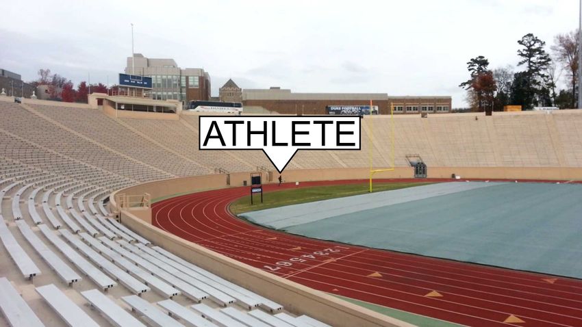
SfM Alignment
this technique, it was important to validate that SfM-derived
models are robust to transient environmental changes. For
example, we generated our stadium model for photos cap-
tured during off hours. In Figure 7, we present an exam-
ple image that aligns accurately to our model, taken during
a well-attended football game. Despite occluded bleachers,
alignment is still feasible as much of the core “structure” of      Figure 8: Illustrating rotational dead reckoning with gy-
the stadium (i.e., the rigid stands, buildings, and boundaries      roscope. As the user follows a moving target, gyroscope
captured in the model) remains visible.                             tracks a rotational matrix “diff” (forward or in reverse in
                                                                    time) from the closest SfM alignment.
Augmenting Vision with Smartphone Sensing. Video
frame-to-model alignment, while quick in FOCUS’ scalable            roscope rotational matrix must first be inverted. Luckily, this
Hadoop-on-cloud pipeline (Section 3.4), is a heavyweight            inversion is trivial: as an invariant, the inverse of a rotation
process. To reduce the computational burden, it is useful           matrix is its transpose.
to combine SfM alignment with inputs from smartphone
sensing. The inertial gyroscope, present on most new smart-         Other smartphone sensors are also valuable during alignment.
phones today, can provide a rotational “diff” across time,          GPS, compass, and accelerometer, can be used to estimate a
in the form of a rotation matrix. By matrix multiplication,         rough camera pose. While these estimates are prone to er-
FOCUS combines this gyroscope-derived rotational matrix             ror, due substantial sources of noise in each sensor, they are
with that of an SfM-estimated camera pose. We illustrate this       valuable to “sanity check” outputs from SfM — immediately
process, akin to a rotational “dead reckoning,” in Figure 8.        rejecting otherwise-silent alignment failures. In these cases,
Of course, errors will accumulate with time, due to inherent        dead reckoning can be applied to overwrite what, otherwise,
noise in the gyroscope sensor. FOCUS periodically re-runs           would be an erroneous alignment result.
SfM alignment, resetting this noise, and maintaining a
bounded inaccuracy (relative to the last frame-to-model             3.2     Quantifying Spatial Content Similarity
alignment). Moreover, since SfM alignment itself is prone to        To cluster video feeds into self-similar groups, FOCUS will
some error, this input from gyroscope can be used to inform         assume a metric to quantify the logical content “similarity.”
hysteresis across multiple alignment attempts.                      Pairs of videos with a high mutual similarity are likely to be
                                                                    placed into the same cluster. As an invariant, each video will
Unsurprisingly, video frame-to-model alignment can fail for         be placed in the cluster with which it has the greatest spatial
several reasons: if the frame is blurred, poorly lit (too dark),    (from line-of-sight) content similarity, averaged across time,
captures sun glare (too bright), the extracted keypoints or fea-    averaged across all other cluster members. In this subsection,
ture descriptors have low correspondence with the model, or         we will present the design of FOCUS’ spatial similarity metric
if the model is too sparse, self-similar, or does not capture the   for a pair of video frames. FOCUS’ metric was not successfully
content of the to-be-aligned frame. In a video stream across        designed “at once;” instead its techniques were evolved and
time, these failures result in alignment “cavities” between suc-    refined through system experimentation.
cessful alignments. To “fill” the cavities, and achieve a con-
tinuous alignment, gyroscope-based dead reckoning is espe-          3.2.1    By Line-of-Sight Intersection (Failed Attempt)
cially useful. Note that dead reckoning is possible in either       FOCUS leverages SfM and gyroscopic tracking to estimate a
direction, forward or backward with time, from the nearest          3D rays of camera pose — originating from the camera and
successful alignment. To dead reckon forward with time, the         along the line-of-sight. For a pair of frames capturing the same
SfM-derived rotational orientation matrix is multiplied with a      object of interest, the corresponding rays should intersect, or
gyroscope-derived rotational matrix, accounting for the rel-        nearly intersect, through the mutual object in view. One pos-
ative rotational motion accumulated over the time interval          sible similarity metric is to consider the shortest distance be-
from the last alignment. To dead reckon in reverse, the gy-         tween these two rays. The resulting 3D line segment must
                                                                    be either (1) between the two points of origin, (2) from the
                                                                    point of origin of one ray to a perpendicular intersection on
                                                                    the other, (3) perpendicular to both rays, or (4) of zero length.
                                                                    We may treat cases (1) and (2) as having no view similarity;
                                                                    line-of-sight rays diverge. In cases (3) and (4), shorter line
                                                                    segments reflect a nearer intersection, and suggest a greater
                                                                    view similarity. Assuming that the constructed rays are ac-
                                                                    curate, this metric is not subject to false negatives; for any
                                                                    pair of videos sharing the same content, the length of the line
                                                                    segment between the rays must be small. Unfortunately, this
                                                                    simple metric is not foolproof. False positive indications of
                                                                    similarity may result; the intended subject may fall in front or
                                                                    behind the point of ray intersection. For example, if stadium
                                                                    spectators in the grandstand focus on different players on the
                                                                    field, this metric will return that the views are similar if the
Figure 7: Challenging example photo that aligns accu-
                                                                    corresponding rays intersect “underground.”
rately to our SfM model (Figure 6), despite capacity at-
tendance (vs. empty during model capture).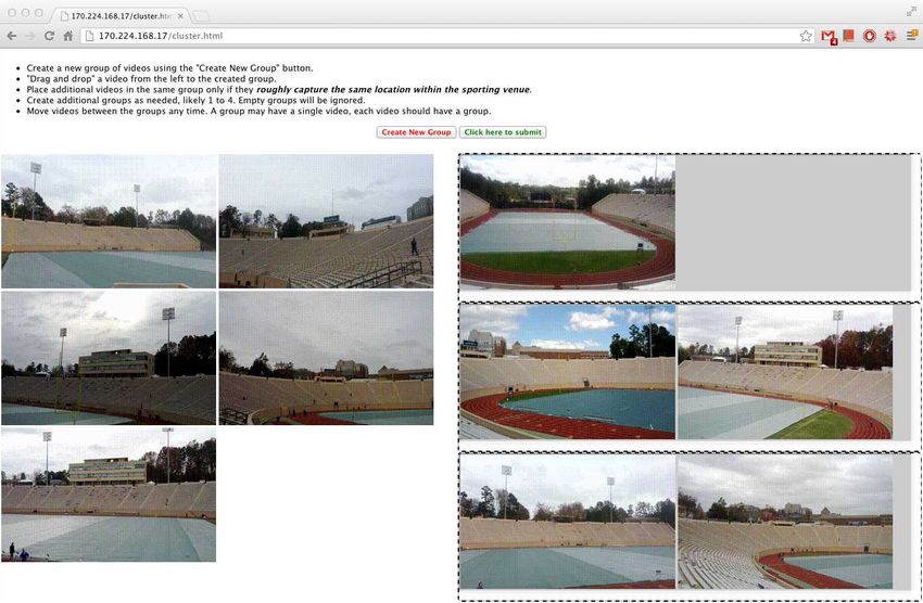
3.2.2    By SfM “Point Cloud” Volumetric Overlap                    perpendicular to one of these planes. Rotation of any 3D
During early experimentation, we found that the above ray-          vector, along a unit-length 3D vector, is given by Rodrigues’
intersection metric, while intuitively appealing in its simplic-    rotation formula. Using this equation, we rotate the O UT
ity, is overly susceptible to false positives. We could eliminate   vector along the R IGHT vector by angle ±(π/2 − vAngle/2)
the potential for false positives by replacing each camera pose     to estimate normals for two planes (top/bottom). Similarly,
ray with a vector, terminating at the object in view. While         rotations along the U P vector with angle ±(π/2 − hAngle/2)
this is difficult to estimate, we can leverage context from the     results in normals to left and right planes. Here, vAngle
3D model structure to terminate the vector roughly “on” the         and hAngles are taken as parameters for the smartphone
model, for example, capturing the ground below the subject.         camera’s field-of-view angle, horizontally and vertically. We
Looking down from a stadium grandstand, subterranean in-            test the signs from these four planar equations for each
tersections would be eliminated. Similarity, intersections in       point in the model, determining the set of points potentially
the air, above the field, can be ignored.                           visible from a particular video frame. Later, we perform set
                                                                    intersections to estimate similarity between the N 2 pairs of
Recall that the SfM model is a point cloud of < x, y, z >           time-synchronized frames of N videos. This N × N value
coordinates, capturing rigid structures. Instead of only con-       table completes our notion of a spatial similarity matrix.
sidering the geometry of a line-of-sight ray, we may identify
structures captured by a video frame. For a pair of videos,         3.3    Clustering by Modularity Maximization
we can compare if both capture the same structures. Sev-            So far, we have discussed what it means for a pair of video
eral techniques from vision apply here. For example, 3D point       frames to be judged “similar,” especially by the intersection
cloud registration heuristics exist for estimating boundaries of    of their respective line-of-sight and field-of-view with an SfM-
a mesh surface, and approximating structures. However, as a         derived 3D model. This notion of “similarity” is a static judg-
simpler, computationally-tractable alternative, we may count        ment, based on an instantaneous point in time. In reality, we
the model points mutually visible in a pair of video frames.        are interested in the similarity of a pair of videos, across multi-
More shared points suggest greater similarity in their views.       ple frames, for some synchronized time interval. This requires
In the next subsection, we discuss how high similarity values,      a further understanding of what it means for a pair of videos
filling an N × N spatial similarity matrix, encourage place-        to be “similar,” above and beyond the similarity of their con-
ment of these videos in the same cluster.                           stituent frames. We will assume that a pair of “similar” video
                                                                    streams need not both track the same spot consistently. In-
To count the number of common points in the intersecting            stead, it is only required that they should both move in a cor-
field-of-views of two videos, we must first isolate the set of      related way, consistently capturing the same physical subject,
points visible in each. As we describe next, the set can be         at the same time. Simply, both streams should maintain (in-
found by considering the pyramid-shaped field-of-view vol-          stantaneous) similarity with each other across time, but not
ume, originating from the camera and expanding with dis-            necessarily have self-similarity from beginning to end. This
tance into the model. Later, we can quickly count the number        seems reasonable in the case of a soccer game: some videos
of shared points across multiple video frames by applying a         will follow the ball, some will follow a favored player, and
quick set intersection. Simply, we construct a bitmap with          others will capture the excitement of the crowd or changes to
each bit representing the presence of one point in the view.1       the scoreboard. These “logical clusters” should map as neatly
The number of shared points can be found by counting the            as possible to FOCUS’ groupings.
number of bits set to 1 in the bitwise AND of two bitmaps.
                                                                    Spatiotemporal Similarity. To capture the mutual corre-
3.2.3    Finding Model Points in a Video View                       spondence in a set of N videos with time, we apply our no-
Let a single estimated line-of-sight be expressed as L(R, t). R     tion of an N × N spatial similarity matrix across T points in
represents a 3×3 rotation matrix, the 3D angle of orientation.      time. For every instant t ∈ T in a synchronized time interval,
t represents a 3 × 1 vector of translation. −R−1 t defines the      we find the corresponding spatial matrix St and apply cluster-
< x, y, z > camera position coordinate, the location in the         ing, finding some set of groupings Gt from line-of-sight and
model from where the video frame was captured. R can be             field-of-view at time t. Next, we aggregate these spatial re-
further decomposed as three row vectors, known respectively         sults into an M = N × N spatialtemporal similarity matrix.
as R IGHT, U P, and O UT, from the perspective of the camera.       Let δg (i, j) = 1 if streams i and j are both placed into the
To capture the camera’s view of the model, we form a pyramid        same spatial cluster g ∈ Gt . δg (i, j) = 0, otherwise.
emerging from the camera position (−R−1 t) and extending in                                    X X
the direction of O UT vector. The four triangular sides of the                          Mij =               δg (i, j)
pyramid are separated, horizontally and vertically, according                                  ∀t∈T ∀g∈Gt
to the camera’s field-of-view (Figure 2).
                                                                    Finally, we apply clustering again, on M , providing groups of
The pyramid-shaped camera view can be abstracted as four            videos matching our notion of spatiotemporal similarity. Next,
planes, all intersecting at the camera position coordinate.         we elaborate on our choice of clustering heuristics.
Now, to fully describe equations for these planes, we must
only find a plane normal vector for each. In order to find four     The “Right” (and Right Number) of Clusters. Several
plane normals, we rotate the O UT vector along the R IGHT           clustering approaches require some parameterization of how
and U P vectors, so that the transformed O UT vector becomes        many clusters are desired (e.g., the k value in k-means clus-
                                                                    tering). By comparison, community identification via modu-
1                                                                   larity maximization has the appealing property that commu-
  Alternatively, Bloom Filters are suitable as probabilistic sub-
stitutes for direct point-to-bit maps, for space-saving bitmaps.    nity boundaries are a function of their modularity, that is, a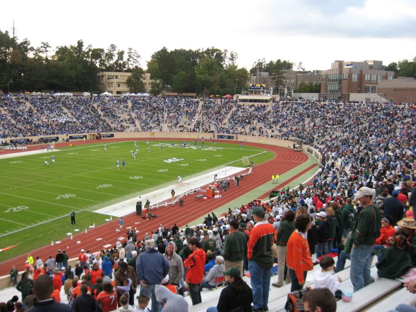
mathematical measure of network division. A network with           streams without requiring computer vision processing or even
high modularity implies that it has high correlation among the     access to video sources. Through iterative design and testing,
members of a cluster and minor correlation with the members        we have refined our technique to be relatively insensitive to
of other clusters. For FOCUS, we apply a weighted modularity       compass error. By considering the wide camera field-of-view
maximization algorithm [13]. As input, FOCUS provides an           angle in the direction of line-of-sight, our metric is not sub-
N × N matrix of “similarity” weights — either that of spatial      stantially impacted by compass errors of comparable angular
or spatiotemporal similarity values. Modularity maximization       size.
returns a set of clusters, each a group of videos, matching our
notions of content similarity.                                     For each latitude/longitude/compass tuple, FOCUS converts
                                                                   the latitude/longitude coordinates to the rectangular Univer-
3.4    Optimizing for Realtime Operation                           sal Transverse Mercator (UTM) coordinate system, taking the
                                                                   E ASTING and N ORTHING value as an < x, y > camera coor-
A key motivation for FOCUS is to provide content analysis          dinate. From the camera, the compass angle is projected to
for streaming realtime content in realtime. Excess computa-        find a 2D line-of-sight ray. Next, two additional rays are con-
tional latency cannot be tolerated as with it increases (1) the    structed, symmetric to and in the same direction as the line
delay before content consumers may be presented with clus-         of sight ray, and separated by the horizontal camera field-
tered videos and (2) the monetary costs of deploying the FO-       of-view (hAngle). This construction can be visualized as a
CUS Hadoop-on-cloud prototype. Here, FOCUS makes two               triangle emerging from the GPS location of a camera and ex-
contributions. First, as previously discussed, FOCUS lever-        panding outward to infinity (with an angle equal to the cam-
ages gyroscope-based dead reckoning as a lightweight proxy         era’s horizontal field-of-view). A metric for view similarity is
to fill gaps between SfM camera pose reconstruction, reduc-        computed as the area bounded by intersecting two such re-
ing the frequency of heavyweight computer vision (alignment        gions. Since this area can be infinite, we impose an additional
of an image to an SfM-derived model) to once in 30 seconds.        bounding box constraint. The resulting metric values are used
Second, FOCUS applies application checkpointing to combat          to populate the spatiotemporal similarity matrix. Clustering
startup latency for SfM alignment tasks.                           proceeds as for SfM-based similarity. To reduce the potential
As described in Section 3.1, FOCUS uses Bundler to align an        for compass error, gyroscope informs a hysteresis across mul-
image (estimate camera pose) relative to a precomputed 3D          tiple compass line-of-sight estimates.
model. Bundler takes approximately 10 minutes to load the          To compute the area of intersection (and thus our metric), we
original model into memory before it can initiate the relatively   find the intersection of the constraining rays with each other
quick alignment optimization process. To avoid this latency,       and with the bounding box, forming the vertices of a sim-
FOCUS uses BLCR [15] to checkpoint the Bundler application         ple (not-self-intersecting) polygon. We may order the vertices
(process) state to disk, just prior to image alignment. The        according to positive orientation (clockwise) by conversion to
process is later restarted with almost zero latency, each time     polar coordinates and sorting by angle. Next, the polygon
substituting the appropriate image for alignment.                  area is found by applying the “Surveyor’s Formula.”

FOCUS Hadoop Prototype Cluster. FOCUS exists as                    4.     EVALUATION
a set of cloud virtual machine instances configured with           Through controlled experimentation2 in two realistic scenarios
Apache Hadoop for MapReduce processing. FOCUS informs              and comparison of FOCUS’ output with human efforts,3 we en-
virtual machine elastic cloud scale-up/down behavior using         deavor to answer the following key questions:
the Hadoop queue size (prototype FOCUS elasticity manager
currently in development). For FOCUS, there are several                 1. How accurate is line-of-sight for identifying unique sub-
types of MapReduce task: (1) base video processing, to                     ject locations? (Figs. 10, 12) Indoors? (Fig. 14) For
include decoding a live video feed and sampling frames for                 objects only a few meters apart? (Figs. 11b, 14b)
further image-based processing; (2) image feature extraction,           2. How does GPS/compass-based line-of-sight estimation
computation of feature descriptors for each keypoint, align-               compare with SfM/gyroscope? (Figures 3, 11, 17)
ment to an SfM model, and output of a bitmap enumerating
                                                                        3. When video streams are misclassified, are incorrectly
the set of visible model points; (3) pairwise image feature
                                                                           clustered videos placed in a reasonable alternative?
matching, used when building an initial 3D SfM model; and
                                                                           Are SfM processing errors silent or overt (enabling our
(4) clustering of similar video feeds. Tasks of multiple types
                                                                           gyroscope-based hysteresis/failover)? (Figs. 12, 13)
may be active simultaneously.
                                                                        4. It our spatiotemporal similarity matrix construction ro-
3.5    Failover to Sensing-only Analysis                                   bust to videos with dynamic, moving content, tracking
                                                                           spatially-diverse subjects with time? (Figure 15)
In certain circumstances, it may be undesirable or infeasible
to use SfM-based line-of-sight estimation. For example, in an           5. What is the latency of vision-based analysis? (Fig. 16)
“iReport” scenario, video may be captured and shared from               6. Is FOCUS’ sensing-only failover approach tolerant to
locations where no SfM model has been previously built. Fur-               large compass errors? Can GPS/compass provide a rea-
ther, users may choose to upload video only if very few peers              sonable accuracy when SfM/gyroscope is undesirable,
are capturing the same video subject — saving battery life and             infeasible, or as temporary failover? (Figures 3, 17)
bandwidth for the user. A lightweight clustering technique,        2
                                                                     Constrained by (a) privacy for video-recording human sub-
without requiring upload of the video stream, could be used        jects and (b) copyright ownership for NCAA athletic events.
to pre-filter uploads of redundant streams. FOCUS provides a       3
                                                                     The procedures for this study were vetted and approved in
sensing-only alternative (using GPS and compass), clustering       advance by our institution’s ethics and legal review board.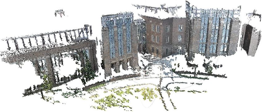
165
East Stand confirm the inferior accuracy of line-of-sight estimation with
132
Scoreboard GPS/compass (only). Note that in both Figures 10 and 11,
West Stand
Distance North of Stadium Center (meters)
a substantial portion of angular “error” is attributable to
99 inaccuracy in filming a designated subjects. Visible outliers
66 in Figure 10 (b) are attributable to poor SfM alignment,
typically due to difficult viewing angles (e.g,. closeups).
33
0 Spatial Clustering Accuracy. Figure 12 summarizes the
accuracy of FOCUS spatial clustering using SfM/gyroscope
−33
in a challenging scenario: clustering on 325 video streams
−66 simultaneously (using sequentially-collected 20-30 second
video clips as a proxy for a large deployment), from the
−99
diverse set of locations shown in Figure 9. FOCUS placed
−132 each “stream” (video clip) in one of three spatial clusters, or
−132 −99 −66 −33 0 33 66 99 132
Distance East of Stadium Center (meters) marked the stream as a processing failure (no SfM alignment,
Figure 9: Experimental locations in/around the stadium. e.g., due to blur). For every assigned member of every spatial
Symbols denote each video’s focal subject: (∗) East Stand; cluster, we compared the video’s intended subject to the
(+) Scoreboard; and (◦) West Stand. geographic centroid of each output cluster. If the assigned
cluster was the closest (geographically) to the intended
7. How do FOCUS’s clusters compare with those created subject, it was considered a “true positive” result (placed
by human volunteers? (Figure 20) in the most correct cluster). Otherwise, it was considered
both a “false negative” for the intended subject and “false
Methodology. Our FOCUS evaluation takes the perspective positive” for its actual placement. Note that we consider false
of a likely use case: user video streams in a collegiate foot- positives/negatives less desirable than processing failures, as
ball stadium and an indoor basketball arena. With 33K seats they represent a silent failure. Sanity checking (by GPS, com-
and a maximum attendance of 56K, by sheer numbers, it is pass, and accelerometer) was not applied. Further, though
likely that multiple (even many) visitors to our stadium would gyroscope-based hysteresis was used in this experiment,
choose to stream video simultaneously. To exercise FOCUS correcting several poor SfM alignments, the short video
across dynamic lighting by time of day, a range of cloud cover, 100
variations in attendance, a span of videographer skill, and
Proportion of Video Streams
90
transient occlusions,4 we collected short video clips from the 80
stadium over a period of two months. 70
60 True Positives
To build the stadium SfM model, containing 190K points and False Positives
50
False Negatives
shown in Figure 6, we took 412 2896x1944 resolution pho- 40 Processing Failures
tographs with a Nikon D3000 SLR camera. All videos were 30
taken in 1920x1088 resolution at 15 FPS, using our Android 20
app, on a Samsung Galaxy Nexus or Galaxy S3. In line-of- 10
0
sight estimation results, short clips (20-30 seconds each) were d rd d ll
tan oa tan era
used. For longer motion tracking results, videographers were s tS or
eb st
S Ov
Ea Sc We
asked to keep the running “athlete” centered in view as con-
sistently as possible, over periods of minutes.
Figure 12: Stadium spatial clustering accuracy. For each
True Positive, FOCUS correctly aligned a video clip and
Line-of-sight Estimation Accuracy. Using our app, three placed it into a cluster with others predominantly captur-
large, preselected points-of-interest in the stadium were ing the same intended subject.
filmed: (1) bleachers where the “pep” band sits, centered
Focus Estimated Subject
in the the E AST S TAND; (2) the press box above mid-field in West Stand N/A
the W EST S TAND; and (3) the S COREBOARD.5 Videographers
walked around arbitrarily, capturing each of the intended
subjects from 325 locations (shown in Figure 9, with locations Scoreboard N/A
from GPS, marked by intended subject). Figures 10 (a,b,c)
show visualizations of SfM/gyroscope-based line-of-sight East Stand N/A
estimation accuracy, for each subject. Dark lines show
estimated line-of-sight. Rough convergence through the
designated subject in the E AST S TAND, S COREBOARD, or d rd d
St
an oa t an
W EST S TAND, respectively, visually suggests that typically st o r eb s tS
Ea Sc We
SfM frame-to-model alignment is highly accurate. Figure 11 True Video Subject
(a,b) plot CDFs, confirming this accuracy. Further, 11 (a,c)
4 Figure 13: Stadium spatial clustering confusion matrix.
For example, an opaque protective tarp not captured by our
SfM model was typically present, covering the entire field. For each intended subject along the X axis, the size of the
5
Large subject areas chosen to reduce impact of human film- circle reflects the proportion of video clips misplaced in
ing error. Figure 11(b) confirms applicability to small subjects. the corresponding Y-axis cluster.165 Cameras pointing toward East Stand 165 Cameras pointing toward Scoreboard 165 Cameras pointing toward West Stand
Distance North of Stadium Center (meters)
Distance North of Stadium Center (meters)
Distance North of Stadium Center (meters)
132 132 132
99 99 99
66 66 66
33 33 33
0 0 0
−33 −33 −33
−66 −66 −66
−99 −99 −99
−132 −132 −132
−132 −99 −66 −33 0 33 66 99 132 −132 −99 −66 −33 0 33 66 99 132 −132 −99 −66 −33 0 33 66 99 132
Distance East of Stadium Center (meters) Distance East of Stadium Center (meters) Distance East of Stadium Center (meters)
Figure 10: Estimated line-of-sight rays on stadium model with true focal subject: (a) in the East Stand; (b) on the
Scoreboard; and (c) in the West Stand. Converging lines reflect precision of SfM line-of-sight estimation.
1 1 1
0.9 0.9 0.9
Proportion of GPS/Compass LoS
0.8 0.8 0.8
Proportion of SfM LoS
0.7 0.7 0.7
Proportion of LoS
0.6 0.6 0.6
East Stand East Stand
SfM LoS
0.5 0.5 Scoreboard 0.5 Scoreboard
GPS/Compass LoS
West Stand West Stand
0.4 0.4 0.4
0.3 0.3 0.3
0.2 0.2 0.2
0.1 0.1 0.1
0 0 0
0 100 200 300 400 500 600 700 800 0 20 40 60 80 100 120 140 160 0 100 200 300 400 500 600 700 800
Distance, LoS to Subject (meters) Distance, SfM LoS to Subject (meters) Distance, GPS/Compass LoS to Subject (meters)
Figure 11: CDFs of alignment “error.” Y-axis shows the shortest distance from the estimated line-of-sight ray to the
intended subject: (a) SfM/gyroscope versus GPS/compass overall; (b) SfM/gyroscope by subject; (c) GPS/compass by
subject. Note that a nontrivial error proportion is attributable to videographer imprecision.
1 100
Proportion of Video Streams
0.9 90
0.8 80
Proportion of SfM LoS
0.7
70
60 True Positives
0.6
Scoreboard 50 False Positives
0.5 Press Box
Basket 40 False Negatives
0.4
30 Processing Failures
0.3 20
0.2 10
0.1 0
rd x et ll
oa Bo sk era
0 eb es
s Ba Ov
0 1 2 3 4 5 6 7 8 9 10 or Pr
Distance, SfM LoS to Subject (meters) Sc
Figure 14: Indoor performance in a collegiate basketball arena: (a) example image from SfM model generation; (b)
SfM/gyroscope line-of-sight estimation accuracy (110 locations); (c) spatial clustering accuracy.
clip time interval limited opportunities for dead reckoning. ample photo from our SfM model; (b) line-of-sight estimation
Figure 13 presents a confusion matrix showing how false accuracy; and (c) spatial clustering accuracy.
positive/negative cluster assignments were distributed. As
expected, nearer subjects were more frequently confused. Spatiotemporal Clustering. Figure 15 presents a dynamic
Overall results achieve 75% “true positive” success. 19% scenario for FOCUS, tracking four video streams across a pe-
are processing failures, in which case FOCUS would invoke riod of minutes. Each stream is tracking one of two “athletes”
GPS/compass failover (we disabled FOCUS’ failover for this (fit volunteers) on the stadium running track. The athletes ran
experiment to restrict results to SfM/gyroscope exclusively). around the track in opposite directions (clockwise and coun-
terclockwise), crossing paths multiple times. In the figure,
Indoor, Low-light Performance. We tested in a 10K-seat each stream is represented by a marker (4, ◦, +, ∗). Each
basketball arena. Strong performance in this challenging in- grouping along the Y-axis denotes a particular video stream.
door environment, where GPS/compass-based techniques do Along the X-axis, we show markers at every second of a four-
not apply and under relatively low light, demonstrates generic minute video. A dark (black) marker denotes a true positive
applicability across environments. Figure 14 shows: (a) an ex- result: a stream, for the corresponding one-second interval,1
was placed in the same spatial cluster as was the true videog-
0.9
rapher intent (same as that of symbol along Y-axis). A light
(red) marker denotes a false positive result: a stream, for the 0.8
Proportion of Operations
corresponding one-second interval, was placed in the same 0.7
spatial cluster as that of symbol along the Y-axis, but contra- 0.6
Feature Extraction
dictory to to the true videographer intent. The figure illus- 0.5
Alignment
trates that, typically, FOCUS is able to place a pair of videos 0.4
with matching content into a matching cluster. It also cap- 0.3
tures all the data required to construct the spatiotemporal 0.2
matrix of content similarity for these clips. The final, over- 0.1
all spatiotemporal clustering successfully outputs the correct 0
stream-to-athlete matching (4 and ◦ grouped for athlete A
0 5 10 15 20 25 30
Processing Latency (seconds)
subject, + and ∗ grouped for athlete B subject). This result Figure 16: CDF of processing latency: video frame feature
was successful even though stream 4 suffered an extended extraction, SfM frame-to-model alignment.
80-second period during which SfM alignment failed (due to
70
deficiencies in our stadium model), leveraging our gyroscope-
Percentage of Streams Misclassified
based dead-reckoning for seamless tracking. 60
50
Computer Vision Computational Latency. FOCUS’ end-
40
to-end performance is largely a function of vision processing,
especially the dominating subtask: alignment of extracted fea- 30
tures to a precomputed SfM model. Figure 16 plots single-
20
threaded performance. In ongoing work, we are investigating
ways to further expedite processing leveraging state-of-the-art 10
techniques for fast alignment [14, 28, 41]. 0
10 20 30 40 50 60
Compass Error, STD (degrees)
Tolerance of Sensing-only Failover to Compass Error.
FOCUS’ sensing-only failover (GPS/compass-based line-of- Figure 17: Box-and-whisker plots showing performance of
sight estimation) must be tolerant to substantial compass GPS/compass-only failover by compass accuracy. X-axis
error. We tested failover by introducing random Gaussian shows standard deviation of introduced Gaussian com-
errors to ground truth compass angles (GPS locations were pass errors (angles in degrees).
used unmodified from experimental locations). Figure 17 User Study: Comparison to Human-created Clusters.
shows diminishing clustering accuracy with extreme compass We recruited 70 volunteers (demographics in Figure 18) to
error, but solid performance with angular error having a compare FOCUS’ clusters to human groupings. Participants
standard deviation of 20 degrees, clustering at 85% accuracy. manually formed clusters from 10 randomly-selected videos
(either from the football stadium or basketball arena datasets)
by “dragging-and-dropping” them into bins, as shown by the
screenshot in Figure 19. We adapt metrics from informa-
∗ tion retrieval to quantify the correctness of both human and
FOCUS-created clusters: precision, recall, and fallout, using
predefined labels of videographer intent.
!
For understanding, precision roughly captures how consis-
tently a volunteer or FOCUS is able to create groupings where
+ each member of the group is a video of the same intended
subject as all other members. Recall captures how completely
a group includes all videos of the same intended subject. Fall-
! out captures how often a video is placed in the same group as
another video that does not capture the same intended subject
0 30 60 90 120 150 180 210 240 (lower values are better). More precisely:
Time (seconds)
Let V = {v1 , v2 , . . . , vn } be a set of videos under test. Let
Video 4 + ◦ ∗ C(vi , vj ) = 1 if vi and vj are placed in the same cluster, 0
4 - 88 151 63 otherwise. Let G(vi , vj ) = 1 if vi and vj should be placed in
+ - 115 149 the same cluster, according to ground truth, 0 otherwise.
◦ - 86
∗ - P RECISION =
|{∀vi , vj ∈ V s.t. G(vi , vj ) ∧ C(vi , vj )}|
|{∀vi , vj ∈ V s.t. C(vi , vj )}|
Figure 15: (a) Y-axis shows four videos, (4) and (◦) cap-
ture athlete A, (+) and (∗) capture B. Markers show R ECALL =
|{∀vi , vj ∈ V s.t. G(vi , vj ) ∧ C(vi , vj )}|
streams placed into the same cluster, by time. Dark mark- |{∀vi , vj ∈ V s.t. G(vi , vj )}|
ers are matching subject. (b) Spatiotemporal matrix M : |{∀vi , vj ∈ V s.t. ¬G(vi , vj ) ∧ C(vi , vj )}|
FALLOUT =
Mij denotes the number of spatial clusters where stream |{∀vi , vj ∈ V s.t. ¬G(vi , vj )}|
i and j were mutually placed.You can also read