The socio-economic determinants of the coronavirus disease (COVID-19) pandemic
←
→
Page content transcription
If your browser does not render page correctly, please read the page content below
The socio-economic determinants of the coronavirus
                                                            disease (COVID-19) pandemic∗
arXiv:2004.07947v6 [physics.soc-ph] 16 May 2020

                                                                                            †
                                                                 Viktor Stojkoski1,2, , Zoran Utkovski3,2, Petar Jolakoski1,
                                                                        Dragan Tevdovski1, and Ljupco Kocarev2,4

                                                         1 Faculty   of Economics, Ss. Cyril and Methodius University in Skopje
                                                                         2 Macedonian Academy of Sciences and Arts
                                                                          3 Fraunhofer Heinrich Hertz Institute, Berlin
                                                                       4 Faculty of Computer Science and Engineering,

                                                                         Ss. Cyril and Methodius University in Skopje
                                                                                                May 19, 2020

                                                                                                   Abstract
                                                            The magnitude of the coronavirus disease (COVID-19) pandemic has an enormous impact
                                                        on the social life and the economic activities in almost every country in the world. Besides the
                                                        biological and epidemiological factors, a multitude of social and economic criteria also gov-
                                                        ern the extent of the coronavirus disease spread in the population. Consequently, there is an
                                                        active debate regarding the critical socio-economic determinants that contribute to the result-
                                                        ing pandemic. In this paper, we contribute towards the resolution of the debate by leveraging
                                                        Bayesian model averaging techniques and country level data to investigate the potential of
                                                        29 determinants, describing a diverse set of socio-economic characteristics, in explaining the
                                                        coronavirus pandemic outcome. We show that the true empirical model behind the coronavirus
                                                        outcome is constituted only of few determinants, but the extent to which each determinant is
                                                        able to provide a credible explanation varies between countries due to their heterogeneous
                                                        socio-economic characteristics. To understand the relationship between the potential determi-
                                                        nants in the specification of the true model, we develop the coronavirus determinants Jointness
                                                        space. In this space, two determinants are connected with each other if they are able to jointly
                                                        explain the coronavirus outcome. As constructed, the obtained map acts as a bridge between
                                                        theoretical investigations and empirical observations, and offers an alternate view for the joint
                                                        importance of the socio-economic determinants when used for developing policies aimed at
                                                        preventing future epidemic crises.
                                                  ∗
                                                      This is a preliminary report.
                                                  †
                                                      Corresponding author: vstojkoski@eccf.ukim.edu.mk

                                                                                                       1
1 Introduction
The coronavirus pandemic began as a simple outbreak in December 2019 in Wuhan, China. How-
ever, it quickly propagated to other countries and became a primary global threat. It seems that
most countries were not prepared for this pandemic. As a consequence, hospitals were over-
crowded with patients and death rates due to the disease skyrocketed. In particular, as of the time
of this writing (10th May 2020), the coronavirus outcome resulted in over 4.2 million cases and
over 280 thousand deaths worldwide as a cause of the induced disease, COVID-191 .
In order to reduce the impact of the disease spread, most governments implemented social dis-
tancing restrictions such as closure of schools, airports, borders, restaurants and shopping malls [1].
In the most severe cases there were even lockdowns – all citizens were prohibited from leaving their
homes. This subsequently lead to a major economic downturn: stock markets plummeted, inter-
national trade slowed down, businesses went bankrupt and people were left unemployed. While
in some countries the implemented restrictions had a significant impact on reducing the expected
shock from the coronavirus, the extent of the disease spread in the population greatly varied from
one economy to another.
A multitude of social and economic criteria have been attributed as potential determinants for
the observed variety in the coronavirus outcome. Some experts say that the hardest hit countries
also had an aging population [2, 3], or an underdeveloped healthcare system [4, 5]. Others empha-
size the role of the natural environment [6, 7]. In addition, while the developments in most of the
countries follow certain common patterns, several countries are notably outliers, both in the num-
ber of officially documented cases and in number of diseased people due to the disease.Having in
mind the ongoing debate, a comprehensive empirical study of the critical socio-economic deter-
minants of the coronavirus epidemic country level outcome would not only provide a glimpse on
their potential impact, but would also offer a guidance for future policies that aim at preventing the
emergence of epidemics.
Motivated by this observation, here we perform a detailed statistical analysis on a large set
of potential socio-economic determinants and explore their potential to explain the variety in the
observed coronavirus cases/deaths among countries. To construct the set of potential determinants
we conduct a thorough review of the literature describing the social and economic factors which
contribute to the spread of an epidemic. We identify a total of 29 potential determinants that
describe a diverse ensemble of social and economic factors, including: healthcare infrastructure,
societal characteristics, economic performance, demographic structure etc. To investigate the per-
formance of each variable in explaining the coronavirus outcome measured either vie the number
of coronavirus cases per million population (p.m.p.) or the number of coronavirus deaths p.m.p.,
we utilize the technique of Bayesian model averaging (BMA). BMA allows us to isolate the most
important determinants by calculating the posterior probability that they truly regulate the process.
At the same time, BMA provides estimates for their relative impact, while also accounting for the
uncertainty in the selection of potential determinants [8–10].
Based on the studied data, we observe patterns which suggest that there are only few determi-
nants that are strongly robust predictors of the coronavirus outcome. As we will discuss in more
detail in the sequel, we observe that some of these factors are related to the effect of size and
influence in social interactions, as well as the investments in health resources. However, the pri-
1 Source: Worldometers coronavirus tracker: https://www.worldometers.info/coronavirus/
2mary analysis does not take into account for the inhomogeneity of the socio-economic nature of
the countries, and thus can not capture (potentially) significant interactions between the potential
determinants. To deal with this problem, we develop the coronavirus determinants Jointness space.
The Jointness space models the interrelation between the potential determinants in explaining the
coronavirus outcome, and acts as a bridge between theoretical investigations and empirical ob-
servations focused at understanding the role of the social and economic factors when developing
policy recommendations for preventing future epidemic crises. Using this space we find that there
may be two efficient routes which can be used for advancing social and economic measures aimed
at preventing the impact of such crises. The first one is by improving the aspects of the healthcare
structure and the natural environment, whereas the second suggest focusing on the societal and
demographic properties. We believe in the absence of realistic models that adequately cover all
relevant aspects, this study provides the first step towards a more comprehensive understanding of
the relationship between the socio-economic determinants of the coronavirus pandemic.
2 Results
2.1 Preliminaries
In a formal setting, both the log of registered COVID-19 cases p.m.p. and the log of COVID-19
deaths p.m.p. are a result of a disease spreading process [11, 12]. The extent to which a disease
spreads within a population is uniquely determined by its reproduction number. This number
describes the expected number of cases directly generated by one case in a population in which
all individuals are susceptible to infection [13, 14]. Obviously, its magnitude depends on various
natural characteristics of the disease, such as its infectivity or the duration of infectiousness [15],
and the social distancing measures imposed by the government [1]. Also, it depends on a plethora
on socio-economic factors that govern the behavioral interactions within a population [16, 17].
In general, we never observe the reproduction number, but rather the disease outcome, i.e.
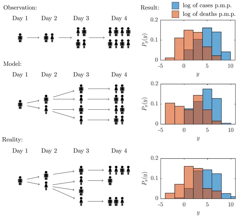
the number of cases/deaths. Fig. 1 depicts qualitatively the differences between the empirical
observations, the mathematical models and the realistic process of the disease spread.
Obviously, it is mathematically complex and computationally expensive to try and infer the
reproduction number. To circumvent this problem we can instead utilize its known characteristics
and derive a much simpler model Mm for the COVID-19 outcome. Here we focus on a specific
formulation where the disease outcome is modeled via a linear regression framework as
yi = β0 + βmT Xm
i + γ si + δ di + ui ,
where we denote both the log of registered COVID-19 cases p.m.p. and the log of COVID-19
deaths p.m.p. of country i as yi . We focus on registered quantities normalized on per capita basis
for the dependent variable instead of raw values to eliminate the bias in the outcomes arising from
the different population sizes in the studied countries. We note that the the observed cases p.m.p.
highly depend on the number of conducted tests in the country. However, the degree of testing also
depends on the potential susceptibility of the population to the virus. Therefore, we argue that both
testing and observed cases p.m.p offer similar information regarding the coronavrius outcome and
exclude the testing variable from our specification. In this aspect, we believe that the deaths p.m.p.
3Figure 1: Qualitative depiction of the differences between the empirical observations, the
mathematical models and the realistic process of COVID-19 spread.
Observation: Each day we observe the total number of registered cases/deaths.
Model: Typically, mathematical models assume a homogeneous spread of the disease, i.e., on average each
person infects the same number of people as quantified through the reproduction number.
Reality: In reality, individuals have different socio-economic characteristics which lead to heterogeneous
susceptibility and infection rates.
Result: The result is the observed histogram based on probability density estimation for the cases and
deaths p.m.p.. The x-axis describes the observed value, whereas the y-axis is the estimated probability
density. We simulate data to generate the histograms for the model and reality situations, whereas the
observation histogram is estimated using country level data.
may provide a more realistic view on the coronavirus outcome because it is solely dependent on
the presence of the disease and the socio-economic interactions between the people in a country.
In the equation, Xmi it is a km dimensional vector of socio-economic explanatory variables that
determine the dependent variable, βm is the vector describing their marginal contributions, β0 is
the intercept of the regression, and ui is the error term. The si term controls for the impact of
social distancing measures of the countries, and γ is its coefficient. Finally, we also include the
term di , with δ capturing its marginal effect, that measures the duration of the epidemics within
the economy. This allows us to control for the possibility that the countries are in a different state
of the disease spreading process.
The linear regression framework is the simplest tool used for quantifying the relationship be-
tween a given outcome and a set of potential determinants. Its advantage lies in the efficient and
unbiased analytical inference of the strength of the linear relationship. In addition it allows us to
use powerful statistical techniques to determine the explanatory power of each independent vari-
4able. As such it has been widely used in modeling of epidemiological phenomena (See for example
Refs. [18–20].
A central question which arises in the model specification is the selection of the independent
variables in Mm . While the literature review offers a comprehensive overview of all potential
determinants, in reality we are never certain of their credibility. To reduce our uncertainty in vari-
able selection, we resort to the technique of Bayesian Model Averaging (BMA). BMA leverages
Bayesian statistics to account for model uncertainty by estimating each possible specification, and
thus evaluating the posterior distribution of each parameter value and probability that a particular
model is the correct one [21].
2.2 Baseline model
The BMA method relies on the estimation of a baseline model M0 that is used for evaluating the
performance of all other models. In our case, M0 is the model which encompasses only the effect
of government social distancing measures and the duration of the epidemics in the country.
We measure the duration of epidemics in a country simply as the number of days since the
first registered case, whereas in order to assess the effect of government restrictions we construct
a stringency index. Mathematically, the index quantifies the average daily variation in government
responses to the epidemic dynamics. As a measure for the daily variation we take the Oxford
Covid-19 stringency index2. The Oxford Covid-19 stringency index is a composite measure that
combines the daily effect of policies on school closures, reduction of internal movement, travel
bans and other similar restrictions. For each country, we construct a weighted average of the
index from all available data since their first registered coronavirus case, up until the last date in
which the daily stringency index is at its maximum value. This threshold is chosen as a means to
capture the moment when a country gains the ability to control and stabilize the propagation of the
disease. To emphasize the effect of policy restrictions implemented on an earlier date in calculating
the average value, we put a larger weight on those dates. This is because earlier restrictions have
obviously a bigger impact on the prevention of the spread of the virus. The procedure implemented
to derive the average government stringency index is described in greater detail in Section S1 of
the Supplementary Material (SM).
Fig 2 visualizes the results from the baseline model. We observe that the countries which had
stringer policies also had less COVID-19 cases and deaths, as expected. In addition, the countries
with longer duration of the crisis registered more cases and deaths per million population.
2.3 Socio-economic determinants
It is apparent that the baseline model can explain only a certain amount of the variations in reg-
istered covid cases/deaths p.m.p.. A fraction of the rest, we believe, can be attributed to various
socio-economic determinants present within a society. To derive the set of potential determinants
we conduct a comprehensive literature review. From the literature review we recognize a total
of 29 potential socio-economic determinants, listed in Table 1. For a detailed description of the
potential effect of the determinants we refer to the references given in the same table, and the
2 More
about the index developed by the Oxford group can be read at
www.bsg.ox.ac.uk/research/publications/variation-government-responses-covid-19
5yi = 3.16 − 0.60si + 0.04di yi = −1.38 − 0.06si + 0.06di
8
R2 = 0.21
R2 = 0.26
8
6
log of deaths p.m.p.
log of cases p.m.p.
6 4
2
4
0
2
-2
0 -4
-2 -1 0 1 -2 -1 0 1
log of government stringency log of government stringency
Figure 2: Explained variation in COVID-19 cases due to government stringency.
references therein. In what follows, we only describe in short the set of potential socio-economic
determinants on the basis of their characteristics.
Healthcare Infrastructure: The healthcare infrastructure essentially determines both the quan-
tity and quality with which health care services are delivered in a time of an epidemic. As measures
for this determinant we include 2 variables which capture the quantity of hospital beds, nurses and
medical practitioners, as well as the quality of the coverage of essential health services. On the one
hand, studies report that well structured healthcare resources positively affect a country’s capacity
to deal with epidemic emergencies [22–29]. On the other hand, the healthcare infrastructure also
greatly impacts the country’s ability to perform testing and reporting when identifying the infected
people. In this regard, economies with better structure are able to easily perform mass testing and
more detailed reporting [30–32].
National health statistics: The physical and mental state of a person play an important role
in the degree to which the individual is susceptible to a disease. In countries where a significant
proportion of the population suffer from diseases highly associated with the spread of an infectious
disease as well as its fatal outcomes, we would expect more severe consequences of the emergent
epidemics [33–36]. Specifically, metabolic disorders such as diabetes may intensify epidemic
complications [37, 38], whereas it has been observed that communicable diseases account for the
majority of deaths in complex emergencies [39]. In addition, there is empirical evidence that
adequate hygiene greatly reduces the rate of mortality [40, 41]. To quantify the national health
characteristics we include 4 variables that assess the general health level in the studied countries.
Economic performance: We evaluate the economic performance of a country through 5 vari-
ables. This performance often mirrors the country’s ability to intervene in a case of a public
health crisis [42–47]. Variables such as GDP per capita have been used in modeling health out-
comes, mortality trends, cause-specific mortality estimation and health system performance and
6finances [48–50]. For poor countries, economic performance appears to improve health by provid-
ing the means to meet essential needs such as food, clean water and shelter, as well access to basic
health care services. However, after a country reaches a certain threshold of development, few
health benefits arise from further economic growth. It has been suggested that this is the reason
why, contrary to expectations, the economic downturns during the 20th century were associated
with declines in mortality rates [51, 52]. Observations indicate that what drives the health in in-
dustrialized countries is not absolute wealth or growth but how the nations resources are shared
across the population [53]. The more egalitarian income distribution within a rich country is asso-
ciated with better health of population [54–57]. Finally, it is also known that in better economies
there are greater trade interactions and people mobility, which may enhance the propagation of an
transmitted disease [17, 22, 47, 58, 59].
Societal characteristics: The characteristics of a society often reveal the way in which people
interact, and thus spread the disease. In this aspect, properties such as education and the degree of
digitalization within a society reflect the level of a person’s reaction and promotion of self-induced
measures for reducing the spread of the disease [60–64]. Governing behavior such as control of
corruption, rule of law or government effectiveness further enhance societal responsibility [65,66].
There are findings which identify the religious view as a critical determinant in the health out-
come [67, 68]. Evidently, the religion drives a person’s attitudes towards cooperation, government,
legal rules, markets, and thriftiness [69]. Finally, the way we mix in society may effectively con-
trol the spread of infectious diseases [17, 59, 70–72]. To measure the societal characteristics we
identify 8 variables.
Demographic structure: Similarly to the national health statistics, the demographic structure
may impact the average susceptibility of the population to a disease. Certain age groups may
simply have weaker defensive health mechanisms to cope with the stress induced by the dis-
ease [73–76]. In addition, the location of living may greatly affect the way in which the disease is
spread [77, 78]. To express these phenomena we collect 6 variables.
Natural environment: A preserved natural environment ensures healthy lives and promotes gen-
eral well-being. Numerous studies indicate that there is a correlation between air pollution and
COVID-19 outcomes [7, 79, 80]. In addition, countries where natural sustainability is deteriorated,
are also more vulnerable to epidemic outbreak [6]. On the other hand, healthy natural environ-
ments may attract more tourists, which could drive the disease spread. We gather the data for 4
variables which capture the essence of this socio-economic characteristic [30].
7Determinant Measure Source Refs.
Healthcare Infrastructure
Medical resources Medical resources index WDI [22–32]
Health coverage UHC service coverage index WDI [22–32]
National health statistics
Death Rate Death rate, crude p.c. WDI [33–36]
Life expectancy Life expectancy at birth WDI [33–36]
Mortality Non-natural causes mortality index WDI [37–41]
Immunization Immunization index WDI [22]
Economic performance
Economic development GDP p.c., PPP $ WDI [42–45, 48–50]
Labor market Employment to population ratio WDI [22, 42, 46, 47]
Government spending Gov. health spending p.c., PPP $ WDI [30, 42–45]
Income inequality GINI index WDI [53–57]
Trade Trade (% of GDP) WDI [22, 47, 58]
Societal characteristics
Social connectedness Social connectedness index (PageRank) DFG [81, 82]
Digitalization Digitalization index WDI [22, 60–64]
Education Human capital index WDI [33, 60–64]
Governance Governance index WGI [65, 66]
Religion 60%+ catholic population NM [67–69]
60%+ christian population NM [67–69]
60%+ muslim population NM [67–69]
Household size Avg. no. of persons in a household UN [17, 59, 70–72]
Demographic structure
Elderly population Population age 65+ (% of total) WDI [73–76]
Young population Population ages 0-14 (% of total) WDI [73–76]
Population size Population, total WM [77, 78]
Rural population Rural population (% of total) WDI [77, 78]
Migration Int. migrant stock (% of population) WDI [77, 78]
Population density People per sq. km WDI [77, 78]
Natural environment
Sustainable development Ecological Footprint (gha/person) GFN [6]
Air Pollution Yearly avg P.M. 2.5 exposure SGA [7, 79, 80]
Air transport Yearly passengers carried WDI [30]
International Tourism Number of tourist arrivals WDI [30]
Table 1: List of Potential determinants of the COVID–19 pandemic.
2.4 BMA estimation
We use this set of determinants and estimate two distinct BMA models. In the first model the de-
pendent variable is the log of COVID-19 cases p.m.p., whereas in the second model we investigate
the critical determinants of the log of the mortality rate due to the coronavirus. The data gathering
8Figure 3: BMA results. Bars for the posterior inclusion probability (PIP), posterior mean (Post. Mean) and
the posterior standard deviation (Post. Std.) of each potential determinant. The determinants are ordered
according to their PIP. The Post. Mean is in absolute value. The signs next to the bar of each determinant
indicate the direction of its impact. The horizontal lines divide the determinants into groups according to
their evidence for being included in the “true” model. Moreover, the horizontal axis is on a logarithmic
scale. The setup used to estimate the results is described in SM Section S3.
and preprocessing procedure is described in SM Section S2, whereas the mathematical background
of BMA together with our inference setup is given in SM Section S3.
Fig. 3 displays the respective results. In both situations, the determinants are ordered according
to their posterior inclusion probabilities (PIP), given in the second column. PIP quantifies the pos-
terior probability that a given determinant belongs to the “true” linear regression model. Besides
this statistic, we also provide the the posterior mean (Post mean) and the posterior standard devia-
tion (Post Std). Post mean is an estimate of the average magnitude of the effect of a determinant,
whereas the Post Std evaluates the deviation from this value.
In the inference procedure we assumed that the “true” model of the coronavirus outcome is
a result of the baseline specification and 3 additional variables. Our prior belief stems from the
general observation which suggests that economies are heterogeneous and a small amount of com-
plementing factors may contribute to the extent of the coronavirus spread, while the other potential
determinants may simply behave as substitutes in terms of socio-economic interpretation within a
country3 . This implies that the prior inclusion probability of each potential determinant is around
0.1. We use this attribute, together with the posterior inclusion probability of each determinant, to
divide the determinants into four disjoint groups:
3 Nevertheless, we found that our results do not depend on the prior assumption of the size of the true model.
9Determinants with strong evidence: (PIP > 0.5). The first group describes the determinants
which have by far larger posterior inclusion probability than prior probability, and thus there is
strong evidence to be included in the true model. We find two such variables related to explaining
the coronavirus cases, the population size and the government health expenditure. The population
size is negatively related to the number of registered COVID-19 cases p.m.p., whereas the health
spending shows a positive impact. The government health expenditure remains the only determi-
nant with strong evidence to be a socio-economic determinant of the coronavirus deaths, with a
positive impact.
Determinants with medium evidence: (0.5 ≥ PIP > 0.1). There are no variables for which
there is medium evidence to be a determinant of the coronavirus cases. When looking at the BMA
estimation of COVID-19 deaths we find only one determinant with medium PIP size, the mortality
from non-natural causes which exhibits negative marginal effect.
Determinants with weak evidence: (0.1 ≥PIP> 0.05). These are determinants which have
lower posterior inclusion probability than their prior one, but still may account for some of the
variations in the coronavirus outcome. For the cases per million population there are four such
determinants, the level of social connectedness, the level of economic development, the mortality
from non-natural causes and the number of international tourist arrivals. The first three variables
have a positive Post Mean, whereas the number of international tourist arrivals has a negative Post
Mean. There is one variable with weak evidence for being a true determinant of the observed
COVID-19 deaths: the population size, with positive effect.
Determinants with negligible evidence: (PIP≤ 0.05). All other potential determinants have
negligible evidence to be a true determinant of the coronavirus outcome. In total, we find negligible
evidence for explaining the coronavirus cases in 23 determinants and for explaining the coronavirus
deaths in 26 potential determinants.
The division of the determinants into groups allows us to assess the robustness of each deter-
minant – determinants belonging to a group described with a larger PIP also offer more credible
explanation for the coronavirus outcome. Nonetheless, we point out that although the comparison
between posterior inclusion probabilities and prior inclusion probabilities is a common approach,
its interpretation must be taken with care. As said in [83], even if the posterior inclusion probabil-
ity is lower than the prior inclusion probability for a given variable, it might be that this particular
variable is important to decision makers under certain circumstances. This is exactly the case with
the inhomogeneous nature of the coronavirus dynamics. Therefore, even if useful for presentation
purposes, the mechanical application of a threshold, or a simple comparison between the prior and
the posterior, should often be avoided in practice.
Definitely, there were several countries which were either extremely affected by the coronavirus
or displayed great immunity to the epidemic crisis. These countries are outliers and may greatly
influence our results. To check the robustness of our results against the presence of such data
we implement the following strategy. First, we remove a country from the sample. Then, we
re-perform the BMA procedure with the resulting countries. We repeat this procedure for every
country, and recover the median results for each potential determinant. The results, shown in SM
Section S4, indicate that the findings presented here are valid even in the presence of potential
10outliers. In the same section, we display the economies which contributed most and least to the
credibility of a particular determinant. These are the countries which, when excluded, lead to the
minimum, respectively maximum, posterior inclusion probability of the given determinant. The
investigation suggests that there are multiple countries which are significant contributors to the PIP
value of each determinant, thus indicating that there is indeed heterogeneity in the socio-economic
features of the countries.
2.5 “Jointness space” of the COVID-19 determinants
The next step in deriving the true socio-economic model behind the coronavirus outcome is to find
its dimension, i.e. the number of explanatory variables included in the model. As a measure for
this quantity, BMA provides the posterior size, formally defined as the posterior belief for the true
dimension of the model. We find that, for the coronavirus cases p.m.p. the posterior model size is
2.1 whereas for the coronavirus deaths p.m.p. it is 1.4.
After discovering the model size, we need to specify the explanatory variables. This raises the
issue of how to construct the appropriate model. While the PIP analysis provided a valuable insight
into the overall importance of single determinants, it neglects the interdependence of inclusion and
exclusion of determinants in a same model. A standard approach for resolving this issue is to
conduct a statistical jointness test. The concept of jointness has been introduced within the BMA
framework with the aim to capture dependence between explanatory variables in the posterior dis-
tribution over the model space [84]. By emphasizing dependence and conditioning on a set of one
or more other variables, jointness moves away from marginal measures of variable importance and
investigates the sensitivity of posterior distributions of parameters of interest to dependence across
regressors. For example, if two variables are complementary in their posterior distribution over the
model space, models that either include or exclude both variables together receive relatively more
weight than models where only one variable is present. In our context, jointness tests will allow
us to infer whether two socio-economic determinants are complements, i.e., tend to be included
together in models with high posterior probability, or substitutes, i.e., models with high posterior
probability tend to exclude the joint inclusion of both determinants.
To better understand the properties of the coronavirus outcome, we perform the jointness test
developed by Hofmarcher et al. [85]. Using this test we can estimate a metric between each
pair of determinants and quantify their relationship in a range between −1 and 1. In the two
extremes, −1 indicates that the two determinants behave as perfect substitutes in the true model,
whereas 1 indicates that they are included in the true model together. The resulting jointness metric
between pairs of determinants can be used to construct a network (graph), which we refer to as the
jointness space of the COVID-19 determinants. In this network, the nodes are the potential socio-
economic determinants, whereas the jointness values represent the edge weights. In other words,
two arbitrary determinants are linked with each other by the posterior belief that both of them
belong to the same linear regression model governing the coronavirus outcome.
In theory, many possible factors may cause complementarity between the determinants, such
as national culture [86], the type of healthcare system [87] or political priorities [88]. All of these
are a priori notions of what dimension drives the relatedness between the potential determinants
and assume that there is little flexibility in choosing the correct model. Instead, the jointness
space follows an agnostic approach and uses a data-driven measure, based on the idea that, if
two determinants are related because they offer contrasting information regarding the coronavirus
11Node labels
1. Death rate 6. Econ. development 11. Education 16. Air transport 21. Catholic religion 26. Medical resources
2. Life expectancy 7. Population density 12. Labor market 17. Sus. development 22. Christian religion 27. Immunization
3. Young population 8. Rural population 13. Health coverage 18. Trade 23. Muslim religion 28. Mortality
4. Elderly population 9. Income inequality 14. Migration 19. Gov. spending 24. Governance 29. Soc. connectedness
5. Population size 10. Int. tourism 15. Air pollution 20. Household size 25. Digitalization
Figure 4: Jointness space of the COVID-19 determinants. The color of the edge between a pair of
determinants is proportional to their Jointness metric. To visualize the network we use the Force-Layout
drawing algorithm.
outcome they will tend to be included in the true model in tandem, whereas determinants that give
similar information are less likely to be included together. Hence, the developed network acts
as a bridge between theoretical foundations and empirical observations, and may be used as an
alternate view for the importance of the socio-economic determinants when developing policies
aimed at reducing the impact of epidemic crises.
The networks depicted in Fig. 4 visualizes the jointness space of the determinants included in
our BMA framework. To emphasize the complementarity between the variables, we connect only
determinants with positive jointness. The full description for the procedure implemented for con-
structing the jointness space is given in SM Section S5. In the networks, the determinants which
can be included in multiple models take a more central position, whereas the periphery is consti-
tuted of determinants whose credibility in explaining the coronavirus outcome mostly substitutes
the effect of other variables. We observe that, in both coronavirus cases and coronavirus deaths,
there are two clusters of tightly connected determinants. In the first cluster, given in the lower left
corner of the two networks, the central role plays the government health spending. Moreover, this
cluster is mostly constituted of determinants that describe the natural environment, together with a
mix of some demographic and health statistic variables. In the second cluster the population size
is the critical node, and appears in the middle of the two drawn networks. This cluster is mainly
constituted of determinants that describe societal characteristics and demographic structure.
12The obtained map suggests that there are two routes for the specification of the true linear-
regression model behind the coronavirus outcome. The first one is by utilizing the aspects of the
healthcare structure and the natural environment. The second route is by introducing a statistical
framework for examining the role of demographics and societal characteristics in the coronavirus
outcome. These patterns may be potentially useful for defining policy recommendations in a sub-
sequent phase aimed at reducing the potential impact of future epidemics: improving the features
of the determinants belonging to a same cluster might yield a synergistic effect, thus significantly
reducing the risk of a negative outcome.
3 Discussion
Our analysis suggests that only a handful of socio-economic determinants are able to robustly
explain the extent of the coronavirus pandemic. The two determinants strongly related to the
coronavirus cases are the population size and the government health expenditure. More populated
economies show greater resistance to being infected by the virus, whereas countries with larger
government expenditure display greater susceptibility to the virus infection. Moreover, there is no
determinant strongly related to the coronavirus deaths per million population.
A plentiful of reasons can be used as a possible interpretation for these results. For instance,
it is known that in structured populations, the degree of epidemic spread scales inversely with
population size [89]. This is because, everything else considered, in larger populations it is easier to
identify and target the critical individuals that are susceptible to the disease [90]. It often turns out,
that these are exactly the individuals which are more socially connected [91]. Another plausible
explanation could be as follows. Early in an epidemics, a certain number of cases, let us say U , go
undetected (latent cases). As the government response is relatively centralized (or with centralized
coordination) the governments usually act when the absolute number of observed cases, let us
say D, exceeds a certain threshold. In this sense, D + U can be considered as the initial state of
the epidemics, after which governments start to act. As D + U does not scale accordingly to the
population size, this effectively means that countries with smaller population size tend to act later
in the epidemic (on a relative scale). This is, however, again different for some countries.
In a similar fashion, various explanations can be found for the observed effect of government
health spending, such as the fact that larger government health spending also implies a more de-
veloped economy, which in turn suggests an older population and increased physical mobility.
However, it could also be the case that more larger health spending leads to bigger testing power
and thus providing better evidence for the coronavirus situation. Nevertheless, government health
expenditure can be large due to inflated costs, as in the case of US, and hence does not necessary
reflect the quality of the public health-care system. Also, countries with low health-care expendi-
ture/weaker public health-care system may be aware of their deficiencies and may thus act aggres-
sively/early in the epidemics (as it is the case with most of the Eastern European countries). We
control for the timing and the stringency of the government measures in the model, but probably
some effects may still persist.
Clearly, the exact interpretation of our analysis is predicated on a more detailed background
on the specific socio-economic features within the countries. We observed this characteristic when
we discovered that the “true”’ model of the coronavirus outcome is constituted of only few deter-
minants, but argued that different models may offer a credible explanation for it. In the absence
13of a unifying framework covering the relevant aspects of the interrelation between the potential
determinants, the jointness analysis performed here (and the resulting jointness space) provide the
starting point for the development of a more comprehensive understanding of the socio-economic
factors of the coronavirus pandemic. We believe that with the improved understanding of the dy-
namics of the coronavirus pandemic, the insights obtained from this analysis can influence the
development of appropriate policy recommendations.
References
[1] Neil Ferguson, Daniel Laydon, Gemma Nedjati Gilani, Natsuko Imai, Kylie Ainslie, Marc
Baguelin, Sangeeta Bhatia, Adhiratha Boonyasiri, ZULMA Cucunuba Perez, Gina Cuomo-
Dannenburg, et al. Report 9: Impact of non-pharmaceutical interventions (npis) to reduce
covid19 mortality and healthcare demand. 2020.
[2] William Gardner, David States, and Nicholas Bagley. The coronavirus and the risks to the
elderly in long-term care. Journal of Aging & Social Policy, pages 1–6, 2020.
[3] Carlos Kennedy Tavares Lima, Poliana Moreira de Medeiros Carvalho, Igor de Araújo Silva
Lima, José Victor Alexandre de Oliveira Nunes, Jeferson Seves Saraiva, Ricardo Inácio
de Souza, Claúdio Gleidiston Lima da Silva, and Modesto Leite Rolim Neto. The emo-
tional impact of coronavirus 2019-ncov (new coronavirus disease). Psychiatry Research,
page 112915, 2020.
[4] Janice Hopkins Tanne, Erika Hayasaki, Mark Zastrow, Priyanka Pulla, Paul Smith, and
Acer Garcia Rada. Covid-19: how doctors and healthcare systems are tackling coronavirus
worldwide. Bmj, 368, 2020.
[5] Ehab Mudher Mikhael and Ali Azeez Al-Jumaili. Can developing countries alone face corona
virus? an iraqi situation. Public Health in Practice, page 100004, 2020.
[6] Moreno Di Marco, Michelle L Baker, Peter Daszak, Paul De Barro, Evan A Eskew, Cecile M
Godde, Tom D Harwood, Mario Herrero, Andrew J Hoskins, Erica Johnson, et al. Opin-
ion: Sustainable development must account for pandemic risk. Proceedings of the National
Academy of Sciences, 117(8):3888–3892, 2020.
[7] Xiao Wu, Rachel C Nethery, Benjamin M Sabath, Danielle Braun, and Francesca Dominici.
Exposure to air pollution and covid-19 mortality in the united states. medRxiv, 2020.
[8] Adrian E Raftery, David Madigan, and Jennifer A Hoeting. Bayesian model averaging for
linear regression models. Journal of the American Statistical Association, 92(437):179–191,
1997.
[9] Jennifer A Hoeting, David Madigan, Adrian E Raftery, and Chris T Volinsky. Bayesian model
averaging: a tutorial. Statistical science, pages 382–401, 1999.
[10] Xavier Sala-i Martin, Gernot Doppelhofer, and Ronald I Miller. Determinants of long-term
growth: A bayesian averaging of classical estimates (bace) approach. American economic
review, pages 813–835, 2004.
14[11] Joseph T Wu, Kathy Leung, and Gabriel M Leung. Nowcasting and forecasting the potential
domestic and international spread of the 2019-ncov outbreak originating in wuhan, china: a
modelling study. The Lancet, 395(10225):689–697, 2020.
[12] Adam J Kucharski, Timothy W Russell, Charlie Diamond, Yang Liu, John Edmunds, Sebas-
tian Funk, Rosalind M Eggo, Fiona Sun, Mark Jit, James D Munday, et al. Early dynamics of
transmission and control of covid-19: a mathematical modelling study. The Lancet Infectious
Diseases, 2020.
[13] Norman TJ Bailey et al. The mathematical theory of infectious diseases and its applications.
Charles Griffin & Company Ltd, 5a Crendon Street, High Wycombe, Bucks HP13 6LE.,
1975.
[14] P Van den Driessche and James Watmough. Further notes on the basic reproduction number.
In Mathematical epidemiology, pages 159–178. Springer, 2008.
[15] Ashleigh R Tuite, Amy L Greer, Michael Whelan, Anne-Luise Winter, Brenda Lee, Ping Yan,
Jianhong Wu, Seyed Moghadas, David Buckeridge, Babak Pourbohloul, et al. Estimated
epidemiologic parameters and morbidity associated with pandemic h1n1 influenza. Cmaj,
182(2):131–136, 2010.
[16] Matt J Keeling and Pejman Rohani. Modeling infectious diseases in humans and animals.
Princeton University Press, 2011.
[17] Petra Klepac, Adam J Kucharski, Andrew JK Conlan, Stephen Kissler, Maria Tang, Hannah
Fry, and Julia R Gog. Contacts in context: large-scale setting-specific social mixing matrices
from the bbc pandemic project. medRxiv, 2020.
[18] Youfa Wang and May A Beydoun. The obesity epidemic in the united statesgender, age,
socioeconomic, racial/ethnic, and geographic characteristics: a systematic review and meta-
regression analysis. Epidemiologic reviews, 29(1):6–28, 2007.
[19] Alessandra Fogli and Laura Veldkamp. Germs, social networks and growth. Technical report,
National Bureau of Economic Research, 2012.
[20] Aisling S Carr, Chris R Cardwell, Peter O McCarron, and John McConville. A systematic
review of population based epidemiological studies in myasthenia gravis. BMC neurology,
10(1):46, 2010.
[21] Enrique Moral-Benito. Model averaging in economics: An overview. Journal of Economic
Surveys, 29(1):46–75, 2015.
[22] Stelios H Zanakis, Cecilia Alvarez, and Vivian Li. Socio-economic determinants of hiv/aids
pandemic and nations efficiencies. European Journal of Operational Research, 176(3):1811–
1838, 2007.
[23] Ralf L Itzwerth, C Raina MacIntyre, Smita Shah, and Aileen J Plant. Pandemic influenza
and critical infrastructure dependencies: possible impact on hospitals. Medical journal of
Australia, 185(S10):S70–S72, 2006.
15[24] Richard J Whitley and Arnold S Monto. Seasonal and pandemic influenza preparedness: a
global threat. The Journal of infectious diseases, 194(Supplement 2):S65–S69, 2006.
[25] Robert F Breiman, Abdulsalami Nasidi, Mark A Katz, M Kariuki Njenga, and John Verte-
feuille. Preparedness for highly pathogenic avian influenza pandemic in africa. Emerging
infectious diseases, 13(10):1453, 2007.
[26] B Adini, A Goldberg, R Cohen, and Y Bar-Dayan. Relationship between equipment and
infrastructure for pandemic influenza and performance in an avian flu drill. Emergency
Medicine Journal, 26(11):786–790, 2009.
[27] Andrew L Garrett, Yoon Soo Park, and Irwin Redlener. Mitigating absenteeism in hospital
workers during a pandemic. Disaster medicine and public health preparedness, 3(S2):S141–
S147, 2009.
[28] Hitoshi Oshitani, Taro Kamigaki, and Akira Suzuki. Major issues and challenges of influenza
pandemic preparedness in developing countries. Emerging infectious diseases, 14(6):875,
2008.
[29] Theodora-Ismene Gizelis, Sabrina Karim, Gudrun Østby, and Henrik Urdal. Maternal health
care in the time of ebola: a mixed-method exploration of the impact of the epidemic on
delivery services in monrovia. World Development, 98:169–178, 2017.
[30] Parviez Hosseini, Susanne H Sokolow, Kurt J Vandegrift, A Marm Kilpatrick, and Peter
Daszak. Predictive power of air travel and socio-economic data for early pandemic spread.
PLoS One, 5(9), 2010.
[31] Sandra Crouse Quinn and Supriya Kumar. Health inequalities and infectious disease epi-
demics: a challenge for global health security. Biosecurity and bioterrorism: biodefense
strategy, practice, and science, 12(5):263–273, 2014.
[32] Daniel R Hogan, Gretchen A Stevens, Ahmad Reza Hosseinpoor, and Ties Boerma. Moni-
toring universal health coverage within the sustainable development goals: development and
baseline data for an index of essential health services. The Lancet Global Health, 6(2):e152–
e168, 2018.
[33] Michael Marmot. Social determinants of health inequalities. The lancet, 365(9464):1099–
1104, 2005.
[34] S-C Chen and C-M Liao. Modelling control measures to reduce the impact of pandemic
influenza among schoolchildren. Epidemiology & Infection, 136(8):1035–1045, 2008.
[35] Elaine Kelly. The scourge of asian flu in utero exposure to pandemic influenza and the
development of a cohort of british children. Journal of Human resources, 46(4):669–694,
2011.
[36] Jonathan S Nguyen-Van-Tam and Alan W Hampson. The epidemiology and clinical impact
of pandemic influenza. Vaccine, 21(16):1762–1768, 2003.
16[37] Dieren Susan van, Joline WJ Beulens, Schouw Yvonne T. van der, Diederick E Grobbee, and
Bruce Nealb. The global burden of diabetes and its complications: an emerging pandemic.
European Journal of Cardiovascular Prevention & Rehabilitation, 17(1 suppl):s3–s8, 2010.
[38] Robert Allard, Pascale Leclerc, Claude Tremblay, and Terry-Nan Tannenbaum. Diabetes and
the severity of pandemic influenza a (h1n1) infection. Diabetes care, 33(7):1491–1493, 2010.
[39] Máire A Connolly, Michelle Gayer, Michael J Ryan, Peter Salama, Paul Spiegel, and David L
Heymann. Communicable diseases in complex emergencies: impact and challenges. The
Lancet, 364(9449):1974–1983, 2004.
[40] Carol W Bassim, Gretchen Gibson, Timothy Ward, Brian M Paphides, and Donald J De-
Nucci. Modification of the risk of mortality from pneumonia with oral hygiene care. Journal
of the American Geriatrics Society, 56(9):1601–1607, 2008.
[41] F Müller. Oral hygiene reduces the mortality from aspiration pneumonia in frail elders.
Journal of dental research, 94(3 suppl):14S–16S, 2015.
[42] John Strauss and Duncan Thomas. Health, nutrition, and economic development. Journal of
economic literature, 36(2):766–817, 1998.
[43] Guillem López i Casasnovas, Berta Rivera, Luis Currais, et al. Health and economic growth:
findings and policy implications. Mit Press, 2005.
[44] Jeffrey Sachs. Macroeconomics and health: investing in health for economic development.
World Health Organization, 2001.
[45] Quamrul H Ashraf, Ashley Lester, and David N Weil. When does improving health raise
gdp? NBER macroeconomics annual, 23(1):157–204, 2008.
[46] Peter Wobst and Channing Arndt. Hiv/aids and labor force upgrading in tanzania. World
Development, 32(11):1831–1847, 2004.
[47] Sara Markowitz, Erik Nesson, and Joshua Robinson. The effects of employment on influenza
rates. Technical report, National Bureau of Economic Research, 2010.
[48] Samuel H Preston. The changing relation between mortality and level of economic develop-
ment. Population studies, 29(2):231–248, 1975.
[49] Spencer L James, Paul Gubbins, Christopher JL Murray, and Emmanuela Gakidou. Devel-
oping a comprehensive time series of gdp per capita for 210 countries from 1950 to 2015.
Population health metrics, 10(1):12, 2012.
[50] Hitoshi Nagano, Jose A Puppim de Oliveira, Allan Kardec Barros, and Altair da Silva Costa
Junior. The heart kuznets curve? understanding the relations between economic development
and cardiac conditions. World Development, 132:104953, 2020.
[51] Stephen Bezruchka. The effect of economic recession on population health. Cmaj,
181(5):281–285, 2009.
17[52] José A Tapia Granados and Edward L Ionides. The reversal of the relation between eco-
nomic growth and health progress: Sweden in the 19th and 20th centuries. Journal of health
economics, 27(3):544–563, 2008.
[53] Richard Wilkinson and Kate Pickett. The spirit level. Why equality is better for everyone,
2010.
[54] Majid Ezzati, Ari B Friedman, Sandeep C Kulkarni, and Christopher JL Murray. The reversal
of fortunes: trends in county mortality and cross-county mortality disparities in the united
states. PLoS medicine, 5(4), 2008.
[55] Arjumand Siddiqi and Clyde Hertzman. Towards an epidemiological understanding of the
effects of long-term institutional changes on population health: a case study of canada versus
the usa. Social science & medicine, 64(3):589–603, 2007.
[56] Ichiro Kawachi and Bruce P Kennedy. Income inequality and health: pathways and mecha-
nisms. Health services research, 34(1 Pt 2):215, 1999.
[57] Kim Krisberg. Income inequality: When wealth determines health: Earnings influential as
lifelong social determinant of health, 2016.
[58] Jérôme Adda. Economic activity and the spread of viral diseases: Evidence from high fre-
quency data. The Quarterly Journal of Economics, 131(2):891–941, 2016.
[59] Kiesha Prem, Alex R Cook, and Mark Jit. Projecting social contact matrices in 152 countries
using contact surveys and demographic data. PLoS computational biology, 13(9):e1005697,
2017.
[60] Robert Putnam. Social capital: Measurement and consequences. Canadian journal of policy
research, 2(1):41–51, 2001.
[61] Sherman Folland. Does community social capital contribute to population health? Social
science & medicine, 64(11):2342–2354, 2007.
[62] Chul-Joo Lee and Daniel Kim. A comparative analysis of the validity of us state-and county-
level social capital measures and their associations with population health. Social indicators
research, 111(1):307–326, 2013.
[63] David P Baker, Juan Leon, Emily G Smith Greenaway, John Collins, and Marcela Movit. The
education effect on population health: a reassessment. Population and development review,
37(2):307–332, 2011.
[64] Johan P Mackenbach, Irina Stirbu, Albert-Jan R Roskam, Maartje M Schaap, Gwenn Men-
vielle, Mall Leinsalu, and Anton E Kunst. Socioeconomic inequalities in health in 22 euro-
pean countries. New England journal of medicine, 358(23):2468–2481, 2008.
[65] Elinor Ostrom. Governing the commons: The evolution of institutions for collective action.
Cambridge university press, 1990.
18[66] Jane Mansbridge. The role of the state in governing the commons. Environmental Science &
Policy, 36:8–10, 2014.
[67] Linda M Chatters. Religion and health: Public health research and practice. Annual review
of public health, 21(1):335–367, 2000.
[68] George K Jarvis and Herbert C Northcott. Religion and differences in morbidity and mortal-
ity. Social science & medicine, 25(7):813–824, 1987.
[69] Luigi Guiso, Paola Sapienza, and Luigi Zingales. People’s opium? religion and economic
attitudes. Journal of monetary economics, 50(1):225–282, 2003.
[70] Niel Hens, Girma Minalu Ayele, Nele Goeyvaerts, Marc Aerts, Joel Mossong, John W Ed-
munds, and Philippe Beutels. Estimating the impact of school closure on social mixing
behaviour and the transmission of close contact infections in eight european countries. BMC
infectious diseases, 9(1):187, 2009.
[71] Joël Mossong, Niel Hens, Mark Jit, Philippe Beutels, Kari Auranen, Rafael Mikolajczyk,
Marco Massari, Stefania Salmaso, Gianpaolo Scalia Tomba, Jacco Wallinga, et al. Social
contacts and mixing patterns relevant to the spread of infectious diseases. PLoS medicine,
5(3), 2008.
[72] Alessia Melegaro, Mark Jit, Nigel Gay, Emilio Zagheni, and W John Edmunds. What types
of contacts are important for the spread of infections? using contact survey data to explore
european mixing patterns. Epidemics, 3(3-4):143–151, 2011.
[73] Jacco Wallinga, Peter Teunis, and Mirjam Kretzschmar. Using data on social contacts to esti-
mate age-specific transmission parameters for respiratory-spread infectious agents. American
journal of epidemiology, 164(10):936–944, 2006.
[74] Anton Erkoreka. The spanish influenza pandemic in occidental europe (1918–1920) and
victim age. Influenza and other respiratory viruses, 4(2):81–89, 2010.
[75] Gregory L Armstrong, Laura A Conn, and Robert W Pinner. Trends in infectious disease
mortality in the united states during the 20th century. Jama, 281(1):61–66, 1999.
[76] Martha Ainsworth and Julia Dayton. The impact of the aids epidemic on the health of older
persons in northwestern tanzania. World Development, 31(1):131–148, 2003.
[77] Rossana Mastrandrea, Julie Fournet, and Alain Barrat. Contact patterns in a high school:
a comparison between data collected using wearable sensors, contact diaries and friendship
surveys. PloS one, 10(9), 2015.
[78] Adam J Kucharski, Kin O Kwok, Vivian WI Wei, Benjamin J Cowling, Jonathan M Read,
Justin Lessler, Derek A Cummings, and Steven Riley. The contribution of social behaviour
to the transmission of influenza a in a human population. PLoS pathogens, 10(6), 2014.
[79] AL Braga, A Zanobetti, and J Schwartz. Do respiratory epidemics confound the association
between air pollution and daily deaths? European Respiratory Journal, 16(4):723–728, 2000.
19[80] Karen Clay, Joshua Lewis, and Edson Severnini. Pollution, infectious disease, and mortal-
ity: evidence from the 1918 spanish influenza pandemic. The Journal of Economic History,
78(4):1179–1209, 2018.
[81] Michael Bailey, Rachel Cao, Theresa Kuchler, Johannes Stroebel, and Arlene Wong. Social
connectedness: Measurement, determinants, and effects. Journal of Economic Perspectives,
32(3):259–80, 2018.
[82] Theresa Kuchler, Dominic Russel, and Johannes Stroebel. The geographic spread of covid-
19 correlates with structure of social networks as measured by facebook. Technical report,
National Bureau of Economic Research, 2020.
[83] Enrique Moral-Benito. Determinants of economic growth: a bayesian panel data approach.
Review of Economics and Statistics, 94(2):566–579, 2012.
[84] Gernot Doppelhofer and Melvyn Weeks. Jointness of growth determinants. Journal of Ap-
plied Econometrics, 24(2):209–244, 2009.
[85] Paul Hofmarcher, Jesus Crespo Cuaresma, Bettina Grun, Stefan Humer, and Mathias Moser.
Bivariate jointness measures in bayesian model averaging: solving the conundrum. Journal
of Macroeconomics, 57:150–165, 2018.
[86] Ludwien Meeuwesen, Atie van den Brink-Muinen, and Geert Hofstede. Can dimensions
of national culture predict cross-national differences in medical communication? Patient
education and counseling, 75(1):58–66, 2009.
[87] Elias Mossialos, Martin Wenzl, Robin Osborn, and Dana Sarnak. 2015 international profiles
of health care systems. Canadian Agency for Drugs and Technologies in Health, 2016.
[88] Taylor C Boas and F Daniel Hidalgo. Electoral incentives to combat mosquito-borne ill-
nesses: Experimental evidence from brazil. World Development, 113:89–99, 2019.
[89] Moez Draief, Ayalvadi Ganesh, and Laurent Massoulié. Thresholds for virus spread on
networks. In Proceedings of the 1st international conference on Performance evaluation
methodolgies and tools, pages 51–es, 2006.
[90] Maksim Kitsak, Lazaros K Gallos, Shlomo Havlin, Fredrik Liljeros, Lev Muchnik, H Eugene
Stanley, and Hernán A Makse. Identification of influential spreaders in complex networks.
Nature physics, 6(11):888–893, 2010.
[91] Romualdo Pastor-Satorras and Alessandro Vespignani. Epidemic spreading in scale-free net-
works. Physical review letters, 86(14):3200, 2001.
[92] Seema Vyas and Lilani Kumaranayake. Constructing socio-economic status indices: how to
use principal components analysis. Health policy and planning, 21(6):459–468, 2006.
[93] Phillip Bonacich. Some unique properties of eigenvector centrality. Social networks,
29(4):555–564, 2007.
20You can also read