Modeling the Population Effects of Hypoxia on Atlantic Croaker (Micropogonias undulatus) in the Northwestern Gulf of Mexico: Part 1-Model ...
←
→
Page content transcription
If your browser does not render page correctly, please read the page content below
Estuaries and Coasts
DOI 10.1007/s12237-017-0266-6

Modeling the Population Effects of Hypoxia on Atlantic Croaker
(Micropogonias undulatus) in the Northwestern Gulf of Mexico:
Part 1—Model Description and Idealized Hypoxia
Kenneth A. Rose 1,2 & Sean Creekmore 1 & Peter Thomas 3 & J. Kevin Craig 4 &
Md Saydur Rahman 5 & Rachael Miller Neilan 6

Received: 30 October 2016 / Revised: 22 April 2017 / Accepted: 21 May 2017
# The Author(s) 2017. This article is an open access publication

Abstract We developed a spatially explicit, individual-based               avoidance of low DO. Hypoxia effects were imposed using
model to analyze how hypoxia effects on reproduction, growth,              exposure effect submodels that converted time-varying expo-
and mortality of Atlantic croaker in the northwestern Gulf of              sures to low DO to reduced hourly growth, increased hourly
Mexico lead to population-level responses. The model follows               mortality, and reduced annual fecundity. Results showed that
the hourly growth, mortality, reproduction, and movement of                100 years of either mild or intermediate hypoxia produced small
individuals on a 300 × 800 spatial grid of 1-km2 cells for                 reductions in population abundance, while repeated severe hyp-
140 years. Chlorophyll-a concentration, water temperature,                 oxia caused a 19% reduction in long-term population abun-
and dissolved oxygen (DO) were specified daily for each grid               dance. Relatively few individuals were exposed to low DO each
cell and repeated for each year of the simulation. A bioenergetics         hour, but many individuals experienced some exposure. The
model was used to represent growth, mortality was assumed                  response was dominated by a 5% average reduction in annual
stage- and age-dependent, and the movement behavior of juve-               fecundity of individuals. Under conditions of random sequences
niles and adults was modeled based on temperature and                      of mild, intermediate, and severe hypoxia years occurring in
                                                                           proportion to their historical frequency, the model predicted a
                                                                           10% decrease in the long-term population abundance of croaker.
Communicated by Dennis Swaney
                                                                           A companion paper substitutes hourly DO values from a three-
Electronic supplementary material The online version of this article       dimensional water quality model for the idealized hypoxia and
(doi:10.1007/s12237-017-0266-6) contains supplementary material,
which is available to authorized users.
                                                                           results in a more realistic population reduction of about 25%.

* Kenneth A. Rose                                                          Keywords Hypoxia . Population . Croaker . Individual-based
  krose@umces.edu                                                          model . Gulf of Mexico

1
    Department of Oceanography and Coastal Sciences, Louisiana State
    University, Baton Rouge, LA 70803, USA
                                                                           Introduction
2
    Present address: Horn Point Laboratory, University of Maryland
    Center for Environmental Science, PO Box 775,
                                                                           Anthropogenic eutrophication is increasing in coastal waters
    Cambridge, MD 21613, USA                                               (Howarth et al. 2011) and has been implicated in causing
3
    Marine Science Institute, University of Texas at Austin, 750 Channel
                                                                           changes to the ecological structure and functioning of semi-
    View Drive, Port Aransas, TX 78373, USA                                enclosed and coastal marine systems (Diaz and Rosenberg
4
    National Oceanic and Atmospheric Administration, National Marine
                                                                           2008). Ecosystem responses to eutrophication include shifts
    Fisheries Service Southeast Fisheries Science Center, Beaufort         in energy flow among functional groups within the food web,
    Laboratory, 101 Pivers Island Road, Beaufort, NC 28516, USA            changes in phytoplankton and fish community composition,
5
    School of Earth, Environmental, and Marine Sciences, University of     declines in habitat quality for fish and other organisms, and
    Texas Rio Grande Valley, Brownsville, TX 78520, USA                    increases in harmful algal blooms (Cloern 2001; Rabalais
6
    Department of Mathematics and Computer Science, Duquesne               et al. 2002). Coastal hypoxia is commonly defined as dis-
    University, Pittsburgh, PA 15282, USA                                  solved oxygen (DO) concentration less than 2 mg l−1, and is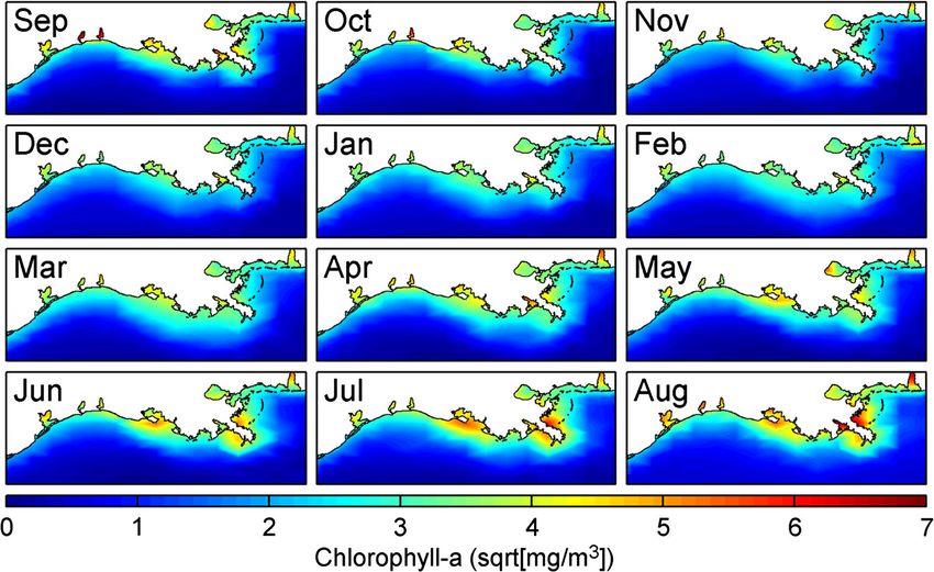
Estuaries and Coasts

often associated with eutrophication. Increasing nutrient load-        Caddy (1993) proposed a conceptual model for how eutro-
ings trigger primary and secondary production that acts as fuel    phication and hypoxia affect fish production. Caddy sug-
to decomposition processes in the bottom layer of stratified       gested that ecosystems reach a point where the negative ef-
water columns (Cloern 2001; Breitburg 2002). However, the          fects of increasing enrichment (including hypoxia) result in
increased secondary production can also stimulate fish pro-        declines of demersal and, eventually, pelagic fish species. In
ductivity (Grimes 2001; Nixon and Buckley 2002; Kemp               a subsequent paper, Caddy (2000) used several case studies
et al. 2005). Efforts to reduce nutrient loadings to coastal wa-   (e.g., Black Sea, Baltic Sea) to illustrate how nutrient loadings
ters are widespread (McCrackin et al. 2017). Eutrophication in     and hypoxia affect fish populations. For example, hypoxia
coastal waters, and associated hypoxia, is expected to increase    effects on the volume of reproductive habitat are one of sev-
in the future due to increased human population and climate        eral major factors implicated in a variety of analyses of Baltic
change (Rabalais et al. 2009).                                     Sea cod recruitment variability (Koster et al. 2005; Margonski
   Hypoxia clearly has detrimental effects on individual fish      et al. 2010; Tomczak et al. 2012; Casini et al. 2016). In another
and on small spatial and temporal scales (i.e., localized ef-      study, Huang et al. (2010) estimated that an average 13%
fects). For example, laboratory and field experiments have         decline in harvest of brown shrimp in North Carolina estuaries
shown that low DO can alter foraging behavior (Pihl et al.         was attributed to hypoxia.
1992; Baustian et al. 2009), reduce growth rate (McNatt and            However, analyses of long-term fisheries landings and
Rice 2004; Stierhoff et al. 2006), affect sex differentiation      survey data have not found convincing widespread evidence
(Shang et al. 2006), and result in reproductive impairment         of the negative effects of hypoxia on coastal fish populations.
(Thomas and Rahman 2009, 2012; Thomas et al. 2007,                 Breitburg et al. (2009a, b) analyzed the landings, nutrient
2015; Murphy et al. 2009; Cheek et al. 2009). In field             loadings, and hypoxia conditions across a suite of estuarine
studies, low DO has been implicated in causing mass                and marine ecosystems and concluded BIt is difficult to find
mortality (Thronson and Quigg 2008), altering spatial dis-         compelling evidence for negative effects of hypoxia on fish-
tributions (Eby and Crowder 2002; Tyler and Targett                eries for mobile species even in systems with extensive and
2007; Switzer et al. 2009; Zhang et al. 2009; Roberts              persistent oxygen depletion if system-wide conditions and to-
et al. 2009; Craig 2012), changing the vertical distribution       tal landings are the focus of analyses.^ Chesney et al. (2000)
and size structure of the zooplankton (Pierson et al. 2009;        and Chesney and Baltz (2001) did not detect any obvious
Roman et al. 2012), and causing a shift in the system              downward trends in long-term fishery-dependent and
from demersal to pelagic species (de Leiva Moreno                  fishery-independent abundance indices for several species in
et al. 2000; Chesney and Baltz 2001).                              Louisiana, and this period included a highly variable but in-
   Knowing the likely ecological consequences of reduc-            creasing trend in hypoxia (see Obenour et al. 2013). An im-
ing nutrients on the system-level is critical to proper            portant caveat is that these statistical (correlative) analyses of
decision-making and public policy formulation (Vaquer-             fisheries time series data have low power to detect an effect at
Sunyer and Duarte 2008; Bianchi et al. 2010; Task Force            the population level given the high degree of variability in the
2015). Reducing nutrient loadings in large coastal systems         available data and other covarying factors (e.g., harvest, cli-
incurs high monetary costs (Butt and Brown 2000;                   mate) that also influence fish population dynamics (Diaz and
Ribaudo et al. 2001; Rabotyagov et al. 2010). There is no          Solow 1999; Chesney and Baltz 2001; Rose et al. 2017).
doubt that reducing hypoxia benefits sessile species and               Analyses based on ecological and population models that
has positive local effects on aquatic fauna, including large       included the Chesapeake Bay, Patuxent Estuary, Gulf of
numbers of individuals (e.g., Roberts et al. 2009; Pollock         Mexico, and the Neuse River (Rose et al. 2009) suggest that
et al. 2007). However, quantitative evidence that reducing         the direct morality effects of hypoxia have small to moderate
hypoxia has positive population-level effects on coastal           effects on fish populations, suggesting that population-level
fish species is equivocal except for several well-studied          responses may result primarily from indirect or sublethal di-
systems (Rose et al. 2009). The reasons that detecting hyp-        rect effects. Likely direct but sublethal effects are reductions in
oxia effects is difficult include high variation in population     growth and reproduction. Indirect effects include displace-
dynamics from other sources, uncertainties in establishing         ment of individuals to inferior habitat or changes in
hypoxia exposure and effects on individuals in the field,          predator-prey interactions that then result in slower growth
and general challenges in monitoring and modeling multi-           or higher mortality. Rose et al. (2009) described a suite of
ple life stages that use different habitats (Rose 2000; Rose       population and community models used to investigate the
et al. 2017a). We use the term Bpopulation level^ here in          effects of hypoxia. They concluded that the modeling evi-
the fisheries management sense of a fish stock: a stock is a       dence suggests that direct effects of hypoxia on coastal fish
group of reproducing individuals of the same species (at           populations are generally small in most years; however, indi-
least semi-closed) that have similar life history parameters       rect effects coupled with the direct effects can result in large
(Begg and Waldman 1999).                                           population-level responses under certain environmental and
Estuaries and Coasts

biological conditions. Rose et al. (2009) also noted that the       stored prior) and income (energy gained during) spawning
seemingly small population-level responses to hypoxia pre-          (see McBride et al. 2015). Eggs, yolk-sac larvae, and ocean
dicted by the reviewed models may reflect the failure to in-        larvae are transported from offshore to nearshore waters dur-
clude certain direct effects (e.g., reproductive impairment), the   ing late fall and winter (Hansen 1969; Rooker et al. 1998;
challenges dealing with modeling the effects of eutrophication      Baltz and Jones 2003), and arrive in shallow coastal habitats
(which increase fish production), and the high uncertainty in       and in estuaries as estuary larvae (typically 50–60 days of age,
quantifying the degree of exposure to hypoxia. Modeling fish        Table 1). Estuary larvae settle out of the plankton to shallow
population responses to variation in environmental factors in       benthic habitats such as salt marshes and gradually move to
general remains a challenge (Rose 2000).                            deeper estuarine and nearshore waters as they transition to
   In this paper, we present a spatially explicit, individual-      early juveniles. Juveniles begin Bbleeding off^ to the shelf
based population dynamics model of Atlantic croaker                 (i.e., offshore) in early summer, with size-at-emigration
(Micropogonias undulatus) in the northwestern Gulf of               increasing (e.g., 55 mm in March; 85 mm in July) as
Mexico (NWGOM). We use the model to examine the effects             the summer season progresses (Yakupzack et al. 1977).
of hypoxia on population-level responses. Atlantic croaker in       Gonadal development in competent first year-of-life in-
the NWGOM is a good case study for investigating the                dividuals and recrudescence in adults begins in the sum-
population-level effects of hypoxia on a coastal fish species.      mer and early fall (Hansen 1969; White and Chittenden
Atlantic croaker is a demersal, estuarine-dependent                 1977; Sheridan et al. 1984; Thomas et al. 2007).
sciaenid fish that frequently inhabits highly productive            Mortality is highly variable in early stages, and juve-
areas along the Texas-Louisiana shelf that are susceptible          niles and adults are subject to mortality as bycatch in
to hypoxia. Croaker dominate summer and fall surveys of             the shrimp fishery (Diamond et al. 1999, 2000).
groundfish on the Gulf of Mexico shelf and can be consid-           Juvenile and adult croaker consume a variety of benthic
ered as an indicator species for the fish communities off of        meiofauna and macrofauna (Nye et al. 2011).
coastal Louisiana (Monk et al. 2015). Also, a relatively                Potential exposure of croaker to low DO occurs on the
large database has accumulated on laboratory and field              nearshore shelf, typically in waters
Estuaries and Coasts

Table 1 Mortality rate (day−1),
duration (days), entering lengths,   Stage              Mortality             Grid               Duration     Entering length (mm)
and whether off or on the model
grid for the egg, yolk-sac larva,    Egg                0.4984                Off                2
ocean larva, estuary larva, early    Yolk-sac           0.1645                Off                4
juvenile, late juvenile, and adult   Ocean larvae       0.0900                Off                45.5
stages
                                                        LA          TX
                                     Estuary larvae     0.0387      0.0414    Off                    58.5
                                     Early juvenile     0.0233      0.0412    On and
Estuaries and Coasts Fig. 1 Model grid for the northwestern Gulf of Mexico showing the stage, and outside of line a (depths >5 m) as adults. A magnified Louisiana and Texas portions of the grid (denoted by dashed line) and 25 × 25 cell area of the grid (referenced by the solid star) is displayed the areas that individuals are confined to according to life stage. in the lower right corner. Station C6, where DO is commonly monitored, Individuals were restricted to cells: within line a (depths
Estuaries and Coasts
Fig. 3 Snapshots of daily
chlorophyll-a concentrations
(mg m−3; square root-trans-
formed) on the 15th day of each
month used in model simulations
Life Stages was assumed to be September 1. Development through the
egg, yolk-sac larva, ocean larva, and estuary larva stages
Simulated croaker individuals progressed through seven life was based on temperature. Transition between the early juve-
stages (egg, yolk-sac larva, ocean larva, estuary larva, early nile and late juvenile stages was length-dependent (97.5 mm);
juvenile, late juvenile, and adult), and were followed as adults late juveniles became adults when their total length exceeded
until they reached their eighth birthday (the assumed 180 mm (Diamond et al. 1999). Eggs, yolk-sac larvae, ocean
maximum age of croaker; Barger 1985), when they were re- larvae, and estuary larvae were followed as individuals, but
moved from the simulation. The birth date of all individuals were assumed to experience grid-wide averaged daily temper-
atures (i.e., they were not followed in a spatially explicit man-
ner). Upon entering the early juvenile stage, each individual
was assigned a weight and length (32-mm total length (TL)
and 0.28 g), positioned randomly on the 2-D spatial grid, and
then followed hourly as individuals through growth, mortality,
reproduction, and movement through age 7. Early juveniles
(including to their initial placement) were restricted to cells
shallower than 5 m, late juveniles to cells shallower than 20 m,
and adults were restricted to cells deeper than 5 m (lines a and
b in Fig. 1). Individuals were allowed to move to any cells
within their depth restrictions. Because the transition of late
juveniles to adults was length-based, there were some age 1
juveniles (individuals 180 mm in their first year before
September 1).
Numerics
Due to the high spatial (1 km2) and temporal (1 h) resolution
of the model, a super-individual approach was used to ensure
reasonable memory usage and computational times (Scheffer
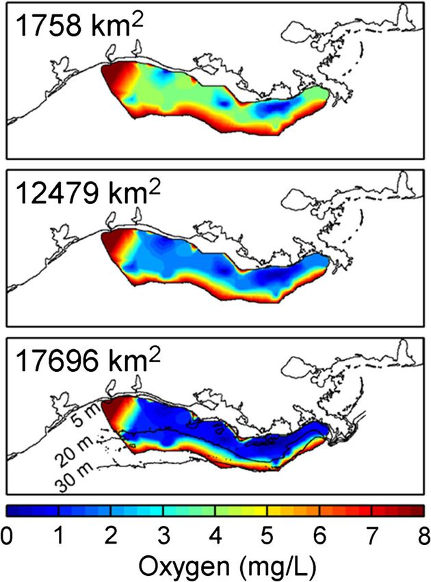
Fig. 4 Maps showing the spatial distribution of DO (mg l−1) for the mild
(top), intermediate (middle), and severe (bottom) hypoxia scenarios used
et al. 1995, ESM-3). This approach follows a fixed number of
in model simulations. Numbers in upper left-hand corner correspond to super-individuals for each age class. Each super-individual is
the areal extent of hypoxia (DOEstuaries and Coasts
population individuals that it represents. Worth is used as a dynamic action, Eg is the egestion, Ex is the excretion, and
weighting factor (in the statistical sense) to scale up from the ρp and ρf are the energy densities (J g−1) of consumed prey and
activities of the super-individual to the population level. of croaker. Maximum consumption and basal respiration rate
Mortality operates to reduce the worth of each super- were computed based on allometric functions of weight and of
individual over time while never actually removing it from temperature. Egestion (Eg) was computed as a fraction of
the population (the same number of super-individuals remains consumption, and SDA and excretion (Ex) were computed as
in the model throughout). When super-individuals reach their fractions of consumption minus egestion. The final parameter
maximum age (age 8), they are removed from the simulated values are shown in Table 2, and the detailed equations are in
population and their places in the computer code are made ESM-4.
available to house newly recruiting early juvenile individuals P-value was computed each hour from the average daily
during the next year. The new early juveniles are the survivors chlorophyll-a concentration Chl in each cell (denoted by col-
that result from all of the eggs released in that year (ESM-3). umn i and row j):
All computations and output variables related to population- " #
level metrics such as abundance, biomass, weight, fecundity, Chli; j
P−valuei; j ¼ 0:8415 þ 0:020⋅ln 3:83 ð3Þ
and spatial distributions are based on an individual’s attributes 52−Chl i; j
multiplied by its worth.
Each hour, a P-value was determined from the chlorophyll-
a concentration in the cell, and daily growth in weight was
Development and Growth computed and divided by 24 to obtain the change in weight for
that hour.
Development of eggs, yolk-sac larvae, ocean larvae, and es- TL (mm) was updated from weight (g) each hour by back-
tuary larvae was temperature-dependent. Each hour, the stage- calculating from the length-weight relationship reported by
specific fractional development FD was computed as follows: Barger (1985):
8
>
> W ¼ 5:302⋅10−6 ⋅TL3:134 ð4Þ
>
> 0:0957⋅e0:06931⋅T ðtÞ ; for eggs
>
>
<
0:0610⋅e0:06931⋅T ðtÞ ; for yolk−sac larvae Individuals could lose weight but not length; maximum
FD ¼ ð1Þ
>
> 0:06931⋅T ðt Þ
weight loss per hour was constrained to no more than 1% of
>
> 0:0045⋅e ; for ocean larvae
>
> their current weight. Weight loss rarely occurred because the
:
0:0082⋅e0:04055⋅T ðtÞ ; for estuary larvae P-values generated using the chlorophyll-a concentrations al-
most always resulted in a positive growth rate and individuals
The grid-wide average daily temperature [T ðt Þ] was used moved every hour frequently to new cells. Length was only
because these life stages were not spatially located in specific updated if the individual was at the weight expected from its
grid cells. The daily temperature was applied for each hour. A length, given the above length-weight relationship (Eq. 4).
running sum of fractional developments was updated each
hour, and when the summed value exceeded one, transition
Mortality
to the next life stage occurred. The same functional form was
used for all stages, but each was calibrated to generate their
Background mortality and starvation-induced mortality, in ad-
target duration (Table 1) when exposed to the grid-wide daily
dition to direct mortality from hypoxia exposure, were repre-
temperatures starting at typical starting dates for each stage.
sented in the model. Background mortality rates (M) were
All super-individuals created as eggs on the same day
specified by life stage and specific to Louisiana and Texas
progressed through the life stages and transitioned to early
estuaries (Table 1). Murphy (2006) modified the mortality
juveniles on the same hour of the same day.
rates reported in Diamond et al. (1999, 2000) based on long-
The growth of individual juvenile and adult croaker under
term field data to separate mortality rates for estuary larvae
normoxia was computed hourly using a bioenergetics model,
and juveniles by Texas versus Louisiana estuaries. Individuals
with the temperature and chlorophyll-a concentration in their
west of 94° longitude (columns 1–200) were assigned Texas
occupied cell. The bioenergetics model followed the
rates, and individuals east of 94° longitude (columns 201–
Wisconsin formulation (Hanson et al. 1997):
800) were assigned Louisiana rates (Fig. 1). All mortality rates
ρp 1 were converted to hourly rates for use in the simulations.
W ðt þ 1Þ ¼ W ðt Þ þ Pvalue⋅C max −ðR þ SDA þ Eg þ ExÞ ⋅W ðt Þ⋅ ⋅
ρ f 24 Starvation occurred when an individual’s weight dropped be-
ð2Þ low 50% of its expected weight based on its length. When a
where P-value is the fraction of maximum consumption super-individual died due to starvation, the individual with all
(Cmax) realized, R is the respiration, SDA is the specific of its worth was removed from the simulation.Estuaries and Coasts Table 2 Parameter values used in the bioenergetics submodel for Symbol Description Values 62 g Atlantic croaker
Estuaries and Coasts

juvenile abundance was determined during calibration. The          Movement
realism of the density-dependent effect on hourly mortality
was assessed by generating spawner-recruit results from the        Hourly movement was modeled using a kinesis algorithm
model and comparing them to reported stock-recruitment re-         (Benhamou and Bovet 1989; Humston et al. 2004), unless
lationships (ESM-5).                                               interrupted by exposure to low DO that triggered avoidance.
                                                                   The position of each juvenile and adult individual was tracked
                                                                   in x-y continuous space (i.e., x and y distances in meters from
Reproduction                                                       the lower left corner of the grid) and in discrete grid space (i.e.,
                                                                   cell number denoted by column i and row j). Kinesis uses the
On September 1 of each year, all individuals were evaluated        velocities of the individual in each of the x and y directions as
for maturity based on their length:                                the sum of two components: an inertial component based on
                                                                   the velocity in the previous hour (I, m h−1) and a randomly
                  1
PM ¼                                                        ð5Þ    generated velocity (D, m h−1):
       1 þ 1:572⋅108 ⋅e−0:1156⋅TL
                                                                   xðt þ 1Þ ¼ xðt Þ þ I x ⋅Δt þ Dx ⋅Δt
Equation 5 results in 70% mature at the typical length of age 1                                                                    ð7Þ
                                                                   yðt þ 1Þ ¼ yðt Þ þ I y ⋅Δt þ Dy ⋅Δt
(about 180 mm) and complete maturity by age 2 (Hansen
1969; Barbieri et al. 1994; Diamond et al. 1999). For each         where Δt is the time step (i.e., 1 h). I and D are shown with x
individual, if a randomly generated value between 0 and 1          and y subscripts to note that separate values are computed for
was less than PM, then that individual was considered mature.      each dimension. The inertial component dominates as the tem-
All mature individuals on September 1 were then assigned a         perature in the occupied cell approaches the optimal tempera-
degree-days value from a triangular probability distribution       ture (Topt), while movement becomes more random under
with minimum, mode, and maximum values (20, 200, and               suboptimal temperature conditions. This approach assumes
450) that determined when they would spawn within the year.        that individuals do not have knowledge of their surrounding
Maturity and the assigned degree-days value were kept by           environment, but can evaluate conditions experienced in the
individuals for the remainder of their life. Every mature indi-    occupied cell relative to some optimum and recall their move-
vidual spawned, but their egg production was multiplied by         ment from the previous time step (Watkins and Rose 2013).
0.5 to account for a 1:1 male to female sex ratio.                    The I and D functions included terms that determined the
   Day of spawning for each individual was determined by its       weighting of the inertial and random components based on
assigned degree-days and its location and movements on the         how close water temperature was to optimal conditions:
grid. Degree-days were computed each day for each mature                           h                       2i
individual starting on September 1 by summing the difference        I ¼ vðt−1Þ⋅h1 ⋅ e−0:5⋅½ðT−T opt Þ=σT
between the temperature in the occupied cell and a specified               h                            2 i                   ð8Þ
temperature threshold (17 °C) below which degree days were          D ¼ ε⋅ 1−h2 ⋅ e−0:5⋅½ðT−T opt Þ=σT
not accumulated. When an individual accumulated its
assigned degree-days, it initiated spawning on that day. Each      where v(t − 1) is the velocity from the previous time step, T is
individual released 12 batches of eggs, one batch every 3 days     water temperature in the occupied cell, Topt is the specified
over a consecutive 34-day period. Assuming that batches can        optimal temperature, and ε is the random swim speed com-
be released every 3–7 days (Waggy et al. 2006), 12 batches         puted as a random deviate from a normal distribution with
would require an individual spawn over 2–3 months, which is        mean equal to distance swum in 1 h (km) at a swimming speed
consistent with Barbieri et al. (1994) for croaker in the          of 3 BL s−1 (i.e., 3·TL · 10−6 ∙ 3600 · Δt) and SD equal to one
Chesapeake Bay. Eggs per batch for each of the 12 batches          half of that distance. The two height parameters (h1 and h2)
were derived from a relationship between weight (W, g) and         and the optimal (Topt) and variance (σT) temperature parame-
potential annual fecundity (F, eggs) reported by Sheridan et al.   ters in Eq. 8 were the same for early juveniles, late juveniles,
(1984):                                                            and adults, but values were specific to certain time periods and
                                                                   were determined by calibration (Table 3). The generated ran-
F ¼ −3248 þ 1179⋅W                                          ð6Þ    dom distance had an equal probability of being positive or
                                                                   negative. Once an individual’s new continuous x and y loca-
Each batch consisted of F/12 eggs multiplied by the worth of       tions were determined, the individual’s cell location was then
the spawning individual. Annual fecundity was recomputed           updated. Early juveniles could only move to cells with depths
using the weight on each day of a batch release during the         less than 5 m, late juveniles to cells with depths less than 20 m,
34 days. The total annual number of eggs spawned by each           and adults to cells with depths greater than 5 m.
individual was the sum of the actual number of eggs spawned           Low DO avoidance behavior was simulated using a thresh-
over all of its batches.                                           old DO level that induced movement with a restricted area
Estuaries and Coasts
Table 3 Description and values of parameters used in the kinesis where DO(t) is the DO concentration in its cell at hour t and
movement model
DONE is the DO threshold below which an effect occurs, and
Symbol Description Value α and β are non-negative constants. The parameters DONE, α,
and β were estimated separately for the growth (fG), reproduc-
Ф Maximum sustained swimming speed (body 3.0 tion (fR), and survival (fS) exposure effect submodels using
lengths s−1)
h1 Height of Gaussian curve for inertial velocity 0.90
published laboratory experiments on spot and croaker
h2 Height of Gaussian curve for random velocity 0.99
(Table 4, ESM-6). The estimated no-effect thresholds
(DONE) were 3.35 mg l−1 for growth, 4.40 for reproduction,
σT Width of Gaussian curves (°C) 3a,c, 4b,d
and 1.35 for mortality.
Topt Optimal temperature (°C) 26a,c, 29b,
21d The values of f from Eq. 9 were then used to determine
hourly reductions in growth and survival (VG and VS), and
a
Apr 16–Jun 15 accumulated and applied once to reduce annual fecundity
b
Jun 16–Sep 15 (VR). For survival, VS was simply set to fS each hour and the
c
Sep 16–Dec 16 worth of an individual was updated using the mortality rate
d
Dec 17–Apr 15 (M) and VS: worth(t + 1) = worth(t) ∙ e−M ∙ Vs. For growth, VG
was updated each hour using fG but with an additional adjust-
ment for repair (sensu Mancini 1983): VG(t + 1) = min(fG,
search (Watkins and Rose 2013). Individuals that entered a VG(t) + 0.21). VG immediately decreased as DO decreased
cell due to kinesis movement with a DO value less than (VG was set to fG each hour), and was limited to increasing
2.0 mg l−1 were assumed to go that cell and then immediately by 0.21 per hour as DO increased. VG was the reduction in
initiate horizontal avoidance behavior (i.e., they moved again instantaneous growth rate and was used to adjust the finite
before any exposure occurred). We used a threshold value of growth rate predicted from Eq. 2. VG and VS were reset to
2.0 mg l−1 to trigger avoidance behavior because croaker in one at the beginning of each year (September 1). For repro-
the NWGOM avoid DO concentrations of 1.2–2.7 mg l−1 duction, VR was computed hourly as the average of the hourly
(Craig 2012). In the hour that avoidance was triggered, indi- fR values over a 10-week period (June 23 to August 31) and
viduals evaluated DO concentrations and temperatures in a then the fecundity of all batches (F in Eq. 6) was multiplied by
neighborhood of cells centered on their current cell and based this final VR value. VR was reset on June 1 to allow for summer
on their length (5 × 5 for 96 to 111 mm, 7 × 7 for 111 to exposure to affect fecundity during the subsequent fall.
140 mm, 9 × 9 for >140 mm). Individuals moved to the center The vitality variables were only imposed on late juve-
of the cell within their neighborhood that had DO >2.0 mg l−1 niles, age 1 adults, and age 2 adults. Early juveniles were
and whose temperature was closest to their Topt. If DO was restricted to the nearshore habitat (Estuaries and Coasts
assigned a weight and length based on the mean length at age hypoxia, each repeated every year. The fourth scenario
relationship (Table 1) and were randomly placed on the grid. consisted of a set of 12 simulations that accounted for inter-
The beginning worth of each super-individual was set to a annual variability in the severity of hypoxia. Twelve randomly
worth specific to its age class, which was based on a specified generated time series sequences of mild, intermediate, and
total worth of entering age 1 individuals (1.5 million) that was severe hypoxia years. In the time series scenario, there was a
then decreased for older ages using the adult mortality rate of 0.18, 0.52, and 0.30 probability of each year being mild, in-
0.0012 day−1. Initial worths by age ranged from 5.92 × 10⁶ for termediate, or severe. The probability of the severity of hyp-
age 1 individuals to 4.28 × 10⁵ for age 7 individuals. The first oxia was estimated by classifying each observed July area of
40 years of all simulations were ignored to minimize any hypoxia (areas noted in Fig. 4) as either mild (20,000 km2)
based on mapping surveys from 1985 to 2010 (Obenour et al.
Design of Simulations 2013).
Calibration Model Outputs
Calibration was performed in a series of steps. First, the de- For all simulations, croaker population dynamics were simu-
velopment rate functions were adjusted using grid-wide aver- lated for 140 years assuming baseline conditions for the first
age daily temperatures until realistic stage durations of egg, 40 years, followed by hypoxic conditions imposed beginning
yolk-sac larva, ocean larva, and estuary larva were obtained in year 41. All model outputs presented are defined in Table 5.
(target values in Table 1). As part of developing a life table for We plotted annual abundance of age 2 and older individuals
croaker, Diamond et al. (1999, 2000) used combinations of over time for all simulations. Results of model calibration are
results reported in laboratory and field data to directly derive shown for the final, full model simulation only. The outputs
stage durations or used entering and exiting lengths, which, for calibration evaluation consisted of mean stage durations,
when combined with growth rates, enabled indirect estimation monthly spatial distributions by life stage, mean lengths at
of durations. Second, bioenergetics parameters were adjusted age, and mean age 2 and older abundance over time.
using the time series of average daily temperatures and as- Aspects of the severe hypoxia applied every year scenario
sumed typical consumption rates (P-values) until average were examined in more detail because while unrealistic, the
stage durations of early and late juveniles and mean length repetition of severe years allowed for clear model responses,
at age of adults were within 5% of target values (Table 1). including lagged effects into future years, to emerge. We used
Third, optimal temperatures and σT values for movement were year 140 as representative of the hypoxia effects having
calibrated by following 1000 super-individuals over 8 years reached steady state at the population level, and show spatial
using the full model (i.e., two-dimensional grid) but without distributions, percent of individuals exposed to low DO aver-
growth and mortality (i.e., individuals followed as moving aged effects (VS, VG, and VR) of the exposed individuals, mean
particles). Fourth, the full model was run with all of the cali- length at age (growth effects), daily mortality, and reproduc-
brated parameter values for 140 years, and final adjustments tion information (percent of age 1 mature, averaged eggs per
were made to ensure that the criteria met with off-grid calibra- batch per individual and per gram). Finally, we examined a
tion were still met in the full model. Finally, the normalizing single replicate of the time series hypoxia simulations and
abundance for density-dependent mortality of late juveniles reported a subset of the outputs reported for the severe
was determined so a stable population of 1.5 million new scenario.
age 1 individuals (i.e., summed worths on September 1 of
their first year) was obtained, which corresponded to a total
adult (entering age 2 and older on September 1) population Results
abundance of about 10 million. Because we simulated an ar-
bitrary population size benchmarked to its own normalizing Calibration and Baseline
abundance for density dependence, all comparisons of hypox-
ia effects were relative to the baseline (normoxic) and other The final baseline simulation showed a stable population
hypoxia simulations. abundance of age 2 and older individuals (top line Fig. 6).
The average abundance during years 101 to 140 was 10 mil-
Hypoxia Scenarios lion and annual egg production averaged 2.19 trillion. The
population stabilized as a result of the calibration and also
Four scenarios of hypoxic conditions were performed using due to the density-dependent mortality of the late juveniles.
the calibrated model. Three scenarios consisted of single sim- Steady-state (but model-generated) recruitment was simulated
ulation each and were the mild, intermediate, or severe to help isolate the effects of hypoxia; in nature, croakerEstuaries and Coasts
Table 5 Model output variables and how they were calculated from the super-individuals
Output variable Calculations
Age 2 and older abundance Computed on September 1 (just after birthdays); youngest individual included as age 2 had one
birthday (age 0 to age 1) and just had their second birthday (age 1 to age 2).
Spatial maps 15th day of each month (June, July, and August); total worth was summed and then summed for
the model cells within coarser cells (10 × 10) for outputting.
Stage durations The duration of each individual as it progressed through egg, yolk-sac, ocean larva, estuary larva,
early juvenile, and late juvenile was recorded and then averaged (weighted by ending worths
of each stage) to obtain single values of averaged stage durations (D ) for each year. Annual
values were then averaged for years 101 to 140.
Mean length (or weight) at age Length (or weight) and worth of each individual entered a new age were recorded, and then
averaged over individuals for each year. Age was reported as the entering age (e.g., mean
length at age 2 was individuals that have lived 2 years—just turned age 2).
Fraction of age 1 mature The number of new age 1 individuals on September 1 that were deemed mature divided by the
total number of new age 1, averaged over years 101 to 140.
Egg production (total and by age) Summed eggs spawned by all individual spawners each year, and averaged over years 101 to
140.
Mean eggs per batch per gram (EPG) and mean eggs Each day, the abundance (summed worths) and biomass (SSB, summed worths times weights) of
per batch per individual (EPI) individuals that spawned, and the summed eggs spawned by these spawners, were recorded by
their age class. For each year, these values were summed to single annual values by age, and
then, EPG and EPI were computed for each year (total eggs per batch/SSB and total eggs per
batch/abundance) and then averaged over years 101 to 140.
Exposure Average percent of surviving age 1 and age 2 individuals on September 1 of year 140 that had
experienced at least 1 h of DOEstuaries and Coasts
12
percentage of individuals exposed to DOEstuaries and Coasts
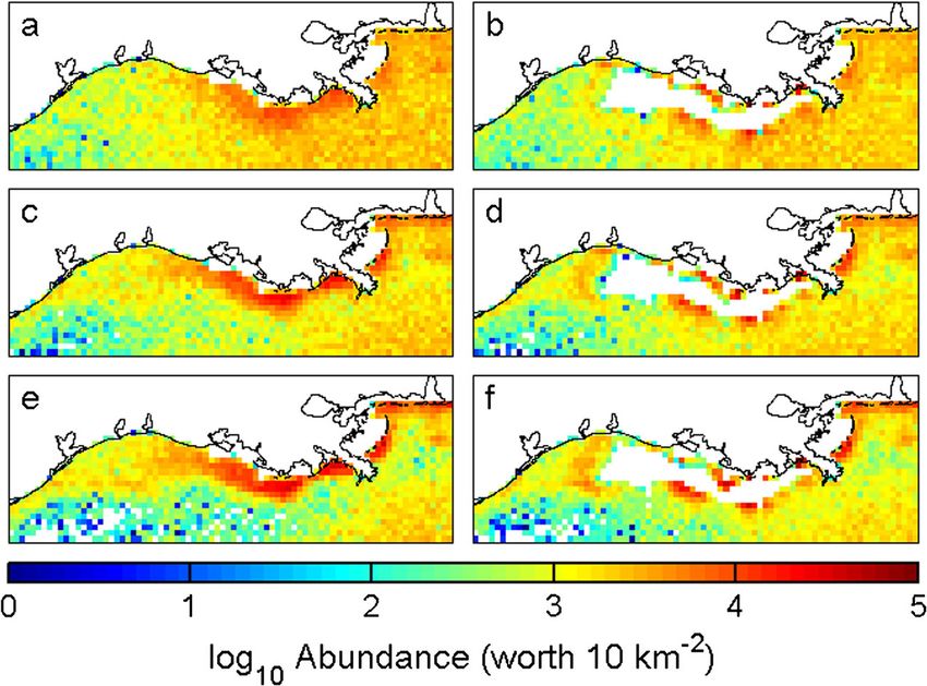
Fig. 7 Mid-monthly snapshots
from model year 140 showing the
spatial distribution of age 2
croaker in the baseline (normoxic)
scenario in a June, c July, and e
August and under the severe
hypoxia scenario in b June, d
July, and f August. Colored pixels
represent the distribution of age 2
croaker abundance (ln-
transformed) based on the inte-
gration of the model 1 × 1-km2
grid cells to a 10 × 10-km2 grid
for mapping
The average of VR culminated in a 20% reduction in average age 2 (97 to 91.4) and age 3 (97.5 to 92.3) individuals. EPI
batch fecundity of exposed individuals in the fall (Fig. 9b, c). decreased by about 8% from the average baseline values for
age 2 (20,446 to 19,064) and age 3 (33,229 to 30,672). Total
Population Responses annual egg production during years 101–140 was, on average,
22% lower (1.708 × 10¹² versus 2.189 × 10¹²) under severe
The effects of severe hypoxia on growth of individual croaker hypoxia.
caused little population-level response, while small and con- Density-dependent mortality in the late juvenile stage
sistent reductions in survival and fecundity of exposed indi- (Fig. 5) offset some of the increased mortality and reduced
viduals that accumulated year after year resulting in the 19% fecundity from exposure to hypoxia. The population declined
reduction in the long-term average abundance of age 2 and slowly each year as late juvenile mortality gradually decreased
older croaker (Fig. 6). While many individuals were exposed from 0.0200 day −1 in year 40 to an average rate of
and those exposed showed lower growth (VG in Fig. 9), few 0.0195 day−1 during years 101–140. These changes in mor-
individuals were exposed for sufficiently long periods of time tality rate resulted in survival of the late juvenile stage increas-
to affect their length (and weight) at age. Mean length at age, ing from 3.6% under baseline to 3.9% after years of exposure
and therefore percentage of age 1 fish that were mature, dif- to severe hypoxia. However, the increased survival of late
fered from baseline by less than 1%. juveniles could only partially offset the hypoxia-induced in-
In contrast, direct mortality due to hypoxia removed a small creased mortality and reduced fecundity of age 1 and age 2
percentage of individuals and reduced fecundity lowered the individuals.
number of eggs per individual of spawners that, when com-
bined, resulted in the nearly 20% reduction at the population Time Series Scenario
level. Average daily mortality rate over years 101–140 for age
1 adults and age 2 adults, and this expressed as the annual When hypoxia was simulated as a random time series of mild,
fraction surviving, increased by about 1% under the severe intermediate, and severe years in proportion to their historical
hypoxia scenario. A 0.5% reduction in annual survival occurrence, the average abundance of age 2 and older croaker
compounded over 40 years results in cumulative reduction abundance for years 101–140 ranged from 88 to 90% of base-
of 20%. The change in age 0 mortality was negligible because line or a reduction of 10–12% (Fig. 10). The relatively small
of low or no exposure of some life stages and lower late amount of variation among replicates in the percentage de-
juveniles leading to density-dependent decreases in mortality cline compared to baseline was because the replicate simula-
rate. Survival of age 3 and older individuals was not affected tions only differed by the random ordering of the mild, inter-
by DO conditions. mediate, and severe hypoxia years.
Reduced reproduction of the exposed individuals led to Reproduction showed a clear decrease due to hypoxia,
reduced EPG and EPI at the population level (Table 6). EPG while annual survival showed a small but persistent response
decreased by about 5% from the average baseline values for and growth showed little change from baseline. Total annualEstuaries and Coasts
25
1.0
(a)
20 (a) 0.8
DO > 1.35
1.35 < DO < 3.35
15 0.6 Mortality (VS)
3.35 < DO < 4.4
Growth (VG)
0.4 Reproduction (VR)
10
0.2
5
0.0
0 June July August
June July August
25 1.0
20 (b) 0.8
Exposure (%)
Effects
15 0.6
0.4
10
0.2 (b)
5
0.0
0 June July August
June July August
25 1.0
(c)
20 0.8
(c)
15 0.6
0.4
10
0.2
5
0.0
0 June July August
June July August Day of Year
Day of Year Fig. 9 Hourly mean effects (V S = survival, V g = growth,
Fig. 8 Stacked area plots showing the percentage of croaker exposed to Vr = reproduction) from June 1 to August 31 for individuals exposed to
3.35 ≤ DO < 4.4 mg l−1 (white), 1.35 ≤ DO < 3.35 mg l−1 (gray), and DO a DO < 1.35 mg l − 1 , b 1.35 ≤ DO < 3.35 m g l − 1 , an d cEstuaries and Coasts
10 the approach is ideal for isolating any potential population-
level effects of hypoxia, which would then provide a mini-
mum estimate of population effects and also provide informa-
Age-2 and Older (106)
tion on the types of responses to be expected within the model
9
and therefore easier to detect and quantify as more and more
realistic conditions are added to the population model. In a
companion paper (Rose et al. 2017a), we explore population
Baseline
8 Time series hypoxia responses of croaker under increased variability by using DO
Average of time series output from a hydrodynamics-water quality model, perform
sensitivity analysis that varies some key model assumptions
and values of inputs, and also perform simulations that also
7 couple the severity of hypoxia to the availability of food for
0 20 40 60 80 100 120 140
Year croaker. In a third paper (Rose et al. 2017b), we impose inter-
Fig. 10 Annual abundance of age 2 and older croaker in the 12 time annual variability on the simulated croaker population re-
series scenario replicates (the dashed line is the average over the replicate sponse to hypoxia to evaluate the ability of field sampling to
runs). The baseline (black line) age 2 and older total abundance is detect a known population-level effect.
included for reference There are fishery-independent data available for croaker
that could provide the basis for a traditional calibration exer-
biotic (food) conditions. Hypoxia varies in time and space, as cise (Janssen and Heuberger 1995) of tuning our model to
does the spatial distribution of croaker, creating a complicated match features of the interannual variability in the data (e.g.,
situation of time-dependent exposures that then must be relat- coefficient of variation of recruitment). However, previous
ed to growth, mortality, and reproduction effects. The attempts were unsuccessful in relating indices of relative
individual-based approach allows for the history of each indi- abundance and landings of fish species to hypoxia in the
vidual to be followed over time and through space, which was Gulf of Mexico (Chesney and Baltz 2001; Chesney et al.
critical for overlaying movement patterns onto the dynamic 2000) and across many coastal systems (Breitburg et al.
hypoxia and environmental conditions (see Hope et al. 2011). 2009a, b). Thus, calibration of our model to mimic observed
Furthermore, the reproduction effect required the accumula- interannual variability is possible (e.g., add a random variation
tion of exposures over 10 weeks, which would be difficult to to egg mortality rate), although the data would already include
simulate without a Lagrangian-type approach. the hypoxia effects and the results would be simply viewed as
Once we simulated exposure, we used a set of three expo- random variation around the population response to hypoxia.
sure effect submodels to determine effects on the growth, sur- We opted instead to create (albeit idealistic) conditions to
vival, and reproduction of individuals. The exposure effect maximize our ability to isolate and understand how hypoxia
submodels had a strong empirical basis, as they were first effects on individuals scale up to population responses. Our
developed from laboratory data and then tested on fluctuating approach of a constant climate (climatological environmental
DO treatments with multiple species prior to their use in the conditions) allowed for both short-term and long-term (multi-
croaker population model (Neilan and Rose 2014). We repre- generational) population responses to be isolated. Our predic-
sented low DO effects as multipliers of growth and fecundity tions are therefore very limited in terms of true forecasting
because that was sufficient for the purposes of our modeling. (Clark et al. 2001) of likely future croaker population abun-
One could have developed effects of low DO on the compo- dances, and our analysis is best considered as simulation ex-
nents (e.g., food intake, respiration) of growth (Vaquer-Sunyer periments (Peck 2004).
and Duarte 2008); however, many laboratory results report Under the repeated environmental conditions, 100 years of
growth only and there are no feedbacks of croaker on prey either mild or intermediate seasonal hypoxia produced small
in the model so the simpler approach of directly adjusting reductions in population abundance. This was because after
growth is sufficient. Similarly, we have some information on the initial development of hypoxia, most individuals success-
the underlying endocrine mechanisms of how low DO reduces fully avoided the relatively small areas of low DO that caused
fecundity (Thomas and Rahman 2009, 2012) that could be mortality and the costs of brief exposure to mild or interme-
used to derive a submodel (e.g., Murphy et al. 2005), but this diate hypoxia were not particularly strong. In contrast, severe
added complexity is not needed to simulate the population hypoxia caused a 19% reduction in long-term population
responses that depend on croaker size (growth) and fecundity. abundance because low DO extended over much of the habitat
Our use of the same temperature, chlorophyll-a concentra- that croaker typically occupy, and the costs of many individ-
tions (food), and hypoxia conditions (i.e., mild, intermediate, uals to some degree of exposure to sublethal DO concentra-
or severe) year after year is clearly not a realistic simulation of tions resulted in reduced fecundity and to a lesser extent in-
the population dynamics of croaker or of hypoxia. However, creased mortality.Estuaries and Coasts
The population response to repeated severe hypoxia years spawner-recruit relationships. We isolated the DO effect, and
was the result of many individuals exposed briefly to low DO, we made assumptions that erred on the side of low exposure
and then the compounding effect over years of the resulting and realistic effects on individuals, which lead to highly ide-
small immediate increases in mortality rate and lowered an- alized conditions being simulated and some sacrificing of re-
nual fecundity. In any given hour, only about 3–4% of the late alism. We address some of these key assumptions in Rose
juvenile, age 1, and age 2 individuals were exposed to low DO et al. (2017a).
(Estuaries and Coasts
adequate DO but potentially less optimal temperatures and avoidance movement and the role played by growth, mortal-
lower food resources. After individuals avoided hypoxic ity, and reproduction in determining population responses.
areas, movement was determined by kinesis based on optimal
temperatures. Because bottom temperatures typically decrease Acknowledgements Funding for this project was provided by the
with depth and distance from shore during the summer, this National Oceanic and Atmospheric Administration, Center for
Sponsored Coastal Ocean Research (CSCOR), NGOMEX06 grant num-
resulted in aggregations of croaker around the offshore edge ber NA06NOS4780131 (to KAR) and NGOMEX09 grant number
of the hypoxic area where DO was tolerable and temperatures NA09NOS4780179 (to KAR and DJ) awarded through the University
were cooler. A similar shift in distribution to cooler tempera- of Texas. The contribution of JKC was partly supported by the National
tures and aggregation near the edge of the hypoxic zone has Oceanic and Atmospheric Administration (NOAA) Center for Sponsored
Coastal Ocean Research Award Nos. NA09NOS4780186 and
been reported in field studies (Craig and Crowder 2005; Craig NA03NOS4780040. We thank the three anonymous reviewers for their
2012). When we repeated the severe hypoxia simulation but very helpful comments. This is publication number 224 of the NOAA’s
individuals avoided low DO by moving to cells with the CSCOR NGOMEX and CHRP programs.
highest DO (i.e., ignored temperature), age 2 and older abun-
Open Access This article is distributed under the terms of the Creative
dance was reduced by 32% (versus 19%), demonstrating the Commons Attribution 4.0 International License (http://
potential indirect effect of hypoxia of displacement of individ- creativecommons.org/licenses/by/4.0/), which permits unrestricted use,
uals to suboptimal conditions. distribution, and reproduction in any medium, provided you give
We also ignored avoidance behavior related to vertical appropriate credit to the original author(s) and the source, provide a link
to the Creative Commons license, and indicate if changes were made.
movements in the water column based on empirical and 3-D
modeling evidence. The hypoxic zone can range from a thin
lens just off of the bottom to more typically 20–50% of the
References
water column (Rabalais and Turner 2006). In our simulations,
individuals had to swim horizontally to minimize exposure to
Babin, B. 2012. Factors affecting short-term oxygen variability in the
low DO, while higher DO water may be available a few me- northern Gulf of Mexico hypoxic zone. PhD Dissertation,
ters higher in the water column. Hydroacoustic and trawling Louisiana State University, Baton Rouge.
studies indicate that fish biomass, not resolvable to the species Baltz, D.M., and R.F. Jones. 2003. Temporal and spatial patterns on
level, is present in the waters immediately overlaying the top microhabitat use by fishes and decapod crustaceans in a Louisiana
Estuary. Transactions of the American Fisheries Society 132: 662–
of hypoxic layer suggesting vertical avoidance (Hazen et al.
678.
2009; Zhang et al. 2009). Even so, based on an analysis of Barbieri, L.R., M.E. Chittenden, and S.K. Lowerre-Barbieri. 1994.
paired trawls that sampled different portions of the lower wa- Maturity, spawning, and ovarian cycle of Atlantic croaker,
ter column, Craig (2012) found no evidence that croaker Micropogonias undulatus, in the Chesapeake Bay and adjacent
moved vertically to avoid low DO. Using similar movement coastal waters. Fishery Bulletin 92: 671–685.
Barger, L.E. 1985. Age and growth of Atlantic croakers in the northern
dynamics as used here, allowing vertical movement potential- Gulf of Mexico, based on otolith sections. Transactions of the
ly reduced exposure to lethal concentrations, depending on American Fisheries Society 114: 847–850.
error-prone individuals were, but had relatively no effect on Baustian, M.M., J.K. Craig, and N.N. Rabalais. 2009. Effects of summer
the exposure to sublethal concentrations (LaBone 2016). 2003 hypoxia on macrobenthos and Atlantic croaker foraging selec-
While assuming that a two-dimensional environment for tivity in the northern Gulf of Mexico. Journal of Experimental
Marine Biology and Ecology 381: S31–S37.
croaker is a reasonable approximation based on field evidence Begg, G.A., and J.R. Waldman. 1999. An holistic approach to fish stock
(also see Rose et al. 2017a), vertical movement should be identification. Fisheries Research 43: 35–44.
considered for other species that show less fidelity to a demer- Benhamou, S., and P. Bovet. 1989. How animals use their environment: a
sal lifestyle. new look at kinesis. Animal Behaviour 38: 375–383.
Bianchi, T.S., M.A. Allison, P. Chapman, J.H. Cowan, M.J. Dagg, J.W.
Day, S.F. DiMarco, R.D. Hetland, and R. Powell. 2010. Forum: new
approaches to the Gulf hypoxia problem. Eos 91: 173.
Next Steps Breitburg, D.L. 2002. Effects of hypoxia, and the balance between hyp-
oxia and enrichment, on coastal fishes and fisheries. Estuaries 25:
The next step in the population modeling is to address some of 767–781.
the simplifying assumptions in this analysis reported here. In Breitburg, D.L., J.K. Craig, R.S. Fulford, K.A. Rose, W.R. Boyton, D.C.
Brady, B.J. Ciotti, R.J. Diaz, K.D. Friedland, J.D. Hagy III, D.R.
the companion paper (Rose et al. 2017a), we use output from a Hart, A.H. Hines, E.D. Houde, S.E. Kolesar, S.W. Nixon, J.A. Rice,
three-dimensional hydrodynamics-water model to specify dy- D.H. Secor, and T.E. Targett. 2009a. Nutrient enrichment and fish-
namic DO concentrations as input to croaker population mod- eries exploitation: interactive effects on estuarine living resources
el and we covary food availability (chlorophyll-a) and hypox- and their management. Hydrobiologia 629: 31–47.
Breitburg, D.L., D.W. Hondorp, L.A. Davias, and R.J. Diaz. 2009b.
ia to simulate their common source of variation from nutrient Hypoxia, nitrogen, and fisheries: integrating effects across local
loadings. We also perform a sensitivity analysis of key model and global landscapes. Annual Review of Marine Science 1: 329–
assumptions including those that control the effectiveness of 349.Estuaries and Coasts
Butt, A.J., and B.L. Brown. 2000. The cost of nutrient reduction: a case enclosed seas around Europe. ICES Journal of Marine Science 57:
study of Chesapeake Bay. Coastal Management 28: 175–185. 1091–1102.
Caddy, J.F. 1993. Toward a comparative evaluation of human impacts on Diamond, S.L., L.B. Crowder, and L.G. Cowell. 1999. Catch and by-
fishery ecosystems of enclosed and semi-enclosed areas. Reviews in catch: the qualitative effects of fisheries on population vital rates
Fisheries Science 1: 57–95. of Atlantic croaker. Transactions of the American Fisheries
Caddy, J.F. 2000. Marine catchment basin effects versus impacts of fish- Society 128: 1085–1105.
eries on semi-enclosed seas. ICES Journal of Marine Science 57: Diamond, S.L., L.G. Cowell, and L.B. Crowder. 2000. Population effects
628–640. of shrimp trawl bycatch on Atlantic croaker. Canadian Journal of
Casini, M., F. Käll, M. Hansson, M. Plikshs, T. Baranova, O. Karlsson, K. Fisheries and Aquatic Sciences 57: 2010–2021.
Lundström, S. Neuenfeldt, A. Gårdmark, and J. Hjelm. 2016. Diaz, R.J., and A. Solow. 1999. Ecological and economic consequences
Hypoxic areas, density-dependence and food limitation drive the of hypoxia: topic 2 report for the integrated assessment on hypoxia
body condition of a heavily exploited marine fish predator. Royal in the Gulf of Mexico. NOAA Coastal Ocean Program Decision
Society Open Science 3 (10): 160416. Analysis Series No. 16. NOAA Coastal Ocean Program, Silver
Cheek, A.O., C.A. Landry, S.L. Steele, and S. Manning. 2009. Diel hyp- Spring. 45 pp.
oxia in marsh creeks impairs the reproductive capacity of estuarine Diaz, R.J., and R. Rosenberg. 2008. Spreading dead zones and conse-
fish populations. Marine Ecology Progress Series 392: 211–221. quences for marine ecosystems. Science 32: 926–929.
Chesney, E.J., D.M. Baltz, and R.G. Thomas. 2000. Louisiana estuarine Eby, L.A., and L.B. Crowder. 2002. Hypoxia-based habitat compression
and coastal fisheries and habitats: perspective from a fish’s eye view. in the Neuse River Estuary: context-dependent shifts in behavioral
Ecological Applications 10: 350–366. avoidance thresholds. Canadian Journal of Fisheries and Aquatic
Chesney, E.J., and D.M. Baltz. 2001. The effects of hypoxia on the north- Sciences 59: 952–965.
ern Gulf of Mexico coastal ecosystem: a fisheries perspective. In Eby, L.A., L.B. Crowder, C.M. McClellan, C.H. Peterson, and M.J.
Coastal hypoxia: consequences for living resources and ecosystems, Powers. 2005. Habitat degradation from intermittent hypoxia: im-
ed. N.N. Rabalais and R.E. Turner, 321–354. Washington, DC: pacts on demersal fishes. Marine Ecology Progress Series 291: 249–
Coastal American Geophysical Union. 262.
Chittenden, M.E. Jr., and D. Moore. 1977. Composition of the ichthyo- Farrell, A.P., A.K. Gamperl, and I.K. Birtwell. 1998. Prolonged swim-
fauna inhabiting the 110-meter bathymetric contour of the Gulf of ming, recovery and repeat swimming performance of mature
Mexico, Mississippi River to the Rio Grande. Northeast Gulf sockeye salmon Oncorhynchus nerka exposed to moderate hypoxia
Science 1: 106–114. and pentachlorophenol. Journal of Experimental Biology 201:
2183–2193.
Clark, J.S., S.R. Carpenter, M. Barber, S. Collins, A. Dobson, J.A. Foley,
Grimes, C.B. 2001. Fishery production and the Mississippi River dis-
D.M. Lodge, M. Pascual, R. Pielke, W. Pizer, C. Pringle, W.V. Reid,
charge. Fisheries 26: 17–26.
K.A. Rose, O. Sala, W.H. Schlesinger, D.H. Wall, and D. Wear.
Gutherz, E.J. 1976. The northern Gulf of Mexico ground fish fishery,
2001. Ecological forecasts: an emerging imperative. Science 293:
including a brief life history of Atlantic croaker (Micropogonias
657–660.
undulatus). Proceedings of the Gulf and Caribbean Fisheries
Cloern, J.E. 2001. Our evolving conceptual model of the coastal eutro-
Institute 29: 87–101.
phication problem. Marine Ecology Progress Series 210: 223–253.
Hansen, D.J. 1969. Food, growth, migration, reproduction, and abun-
Cole, J., and J. McGlade. 1998. Clupeoid population variability, the en-
dance of pinfish, Lagodon rhomboides, and Atlantic croaker,
vironment and satellite imagery in coastal upwelling systems.
Micropogon undulatus, near Pensacola, Florida, 1963-65. Fishery
Reviews in Fish Biology and Fisheries 8: 445–471.
Bulletin 68: 135–146.
Cowan, J.H. Jr., K.A. Rose, and D.R. DeVries. 2000. Is density- Hanson, P.C., T.B. Johnson, D.E. Schindler, and J.F. Kitchell. 1997. Fish
dependent growth in young-of-the year fishes a question of critical bioenergetics 3.0 for Windows. University of Wisconsin Sea Grant
weight? Reviews in Fish Biology and Fisheries 10: 61–89. Institute, WISCU-T-97-001, Madison.
Craig, J.K. 2012. Aggregation on the edge: effects of hypoxia avoidance Hazen, E.L., J.K. Craig, C.P. Good, and L.B. Crowder. 2009. Vertical
on the spatial distribution of brown shrimp and demersal fishes in distribution of fish biomass in hypoxic waters on the Gulf of
the Northern Gulf of Mexico. Marine Ecology Progress Series 445: Mexico shelf. Marine Ecology Progress Series 375: 195–207.
75–95. Hirst, A.G., and A.J. Bunker. 2003. Growth of marine planktonic cope-
Craig, J.K., and L.B. Crowder. 2005. Hypoxia-induced habitat shifts and pods: global rates and patterns in relation to chlorophyll a, temper-
energetic consequences in Atlantic croaker and brown shrimp on the ature, and body weight. Limnology and Oceanography 48: 1988–
Gulf of Mexico shelf. Marine Ecology Progress Series 294: 79–94. 2010.
Craig, J.K., J.A. Rice, L.B. Crowder, and D.A. Nadeau. 2007. Density- Hope, B.K., W.T. Wickwire, and M.S. Johnson. 2011. The need for in-
dependent growth and mortality in an estuary-dependent fish: an creased acceptance and use of spatially explicit wildlife exposure
experimental approach with juvenile spot Leiostomus xanthurus. models. Integrated Environmental Assessment and Management 7:
Marine Ecology Progress Series 343: 251–262. 156–157.
Craig, J.K., P.C. Gillikin, M.A. Magelnicki, and L.N. May Jr. 2010. Houde, E.D. 2008. Emerging from Hjort’s shadow. Journal of Northwest
Habitat use of cownose rays (Rhinoptera bonasus) in a highly pro- Atlantic Fishery Science 41: 53–70.
ductive, hypoxic continental shelf ecosystem. Fisheries Howarth, R., F. Chan, D.J. Conley, J. Garnier, S.C. Doney, R. Marino,
Oceanography 19: 301–317. and G. Billen. 2011. Coupled biogeochemical cycles: eutrophication
Darnell R.M., J.A. Kleypas, and R.E. Defenbaugh. 1983 Northwestern and hypoxia in temperate estuaries and coastal marine ecosystems.
Gulf Shelf bio-atlas. Minerals Management Service Report 82–04. Frontiers in Ecology and the Environment 9: 18–26.
Minerals Management Service, Gulf of Mexico, OCS Region, New Huang, L., M.D. Smith, and J.K. Craig. 2010. Quantifying the economic
Orleans. effects of hypoxia on a fishery for brown shrimp Farfantepenaeus
Darnell, R.M. 1990. Mapping of the biological resources of the continen- aztecus. Marine and Coastal Fisheries 2: 232–248.
tal shelf. American Zoologist 30: 15–21. Humston, R., D.B. Olson, and J.S. Ault. 2004. Behavioral assumptions in
de Leiva Moreno, J.I., V.N. Agostini, J.F. Caddy, and F. Carocci. 2000. Is models of fish movement and their influence on population dynam-
the pelagic-demersal ratio from fishery landings a useful proxy for ics. Transactions of the American Fisheries Society 133: 1304–
nutrient availability? A preliminary data exploration for the semi- 1328.You can also read