A Machine Learning Approach to Analyze and Support Anti-Corruption Policy 9015 2021
←
→
Page content transcription
If your browser does not render page correctly, please read the page content below
9015
                                                 2021
                                                  April 2021

A Machine Learning Approach
to Analyze and Support Anti-
Corruption Policy
Elliott Ash, Sergio Galletta, Tommaso Giommoni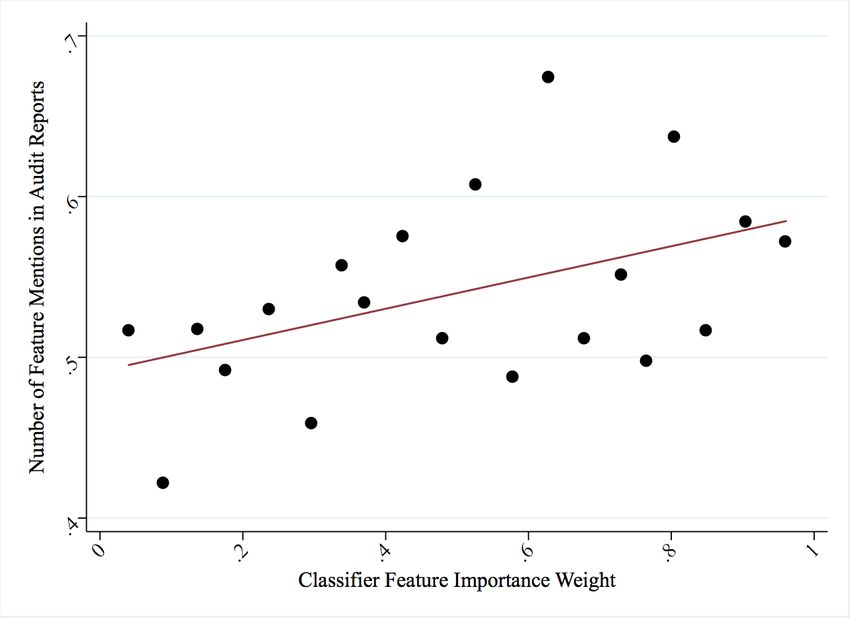
Impressum:

CESifo Working Papers
ISSN 2364-1428 (electronic version)
Publisher and distributor: Munich Society for the Promotion of Economic Research - CESifo
GmbH
The international platform of Ludwigs-Maximilians University’s Center for Economic Studies
and the ifo Institute
Poschingerstr. 5, 81679 Munich, Germany
Telephone +49 (0)89 2180-2740, Telefax +49 (0)89 2180-17845, email office@cesifo.de
Editor: Clemens Fuest
https://www.cesifo.org/en/wp
An electronic version of the paper may be downloaded
· from the SSRN website:       www.SSRN.com
· from the RePEc website:      www.RePEc.org
· from the CESifo website:     https://www.cesifo.org/en/wp
CESifo Working Paper No. 9015

     A Machine Learning Approach to Analyze and
           Support Anti-Corruption Policy

                                          Abstract

Can machine learning support better governance? In the context of Brazilian municipalities,
2001-2012, we have access to detailed accounts of local budgets and audit data on the associated
fiscal corruption. Using the budget variables as predictors, we train a tree-based gradient-
boosted classifier to predict the presence of corruption in held-out test data. The trained model,
when applied to new data, provides a prediction-based measure of corruption that can be used
for new empirical analysis or to support policy responses. We validate the empirical usefulness
of this measure by replicating and extending some previous empirical evidence on corruption
issues in Brazil. We then explore how the predictions can be used to support policies toward
corruption. Our policy simulations show that, relative to the status quo policy of random audits,
a targeted policy guided by the machine predictions could detect almost twice as many corrupt
municipalities for the same audit rate. Similar gains can be achieved for a politically neutral
targeting policy that equalizes audit rates across political parties.
JEL-Codes: D730, E620, K140, K420.
Keywords: algorithmic decision-making, corruption policy, local public finance.

                  Elliott Ash                                     Sergio Galletta
            ETH Zürich / Switzerland                        University of Bergamo / Italy
                ashe@ethz.ch                                 sergio.galletta@unibg.it

                                     Tommaso Giommoni
                                   ETH Zürich / Switzerland
                                      giommoni@ethz.ch

We benefited from comments by participants at seminars at the University of St. Gallen, ETH
Zürich, University of Zürich, the “Advances in Economics Winter Symposium” (Bergamo),
Bonn Law and Economics Workshop, and the Online Workshop in Computational Analysis of
Law. We are grateful to Francisco Cavalcanti for sharing essential data for conducting the
analysis. David Cai, Matteo Pinna, and Angelica Serrano provided excellent research assistance.
Thanks to Daniel Bjorkegren, Aniket Kesari, Himabindu Lakkaraju, Michael Livermore, and
Julian Nyarko for comments on previous drafts.
This version: April 2021 (First version: April 2020).
1. Introduction
A large body of anecdotal and empirical evidence speaks to the deep and negative
impacts of corruption. According to recent United Nations statistics, for example, inter-
national corruption costs the global economy over 3.6 trillion USD annually. On a more
micro level, social scientists have demonstrated that foul play by government actors does
real harm to the average citizen. These harms lead to responses in politics and political
participation (Ferraz and Finan, 2008; Chong et al., 2015), undermine trust toward in-
stitutions (Morris and Klesner, 2010), and have additional side effects on the economy
(Lagaras et al., 2017).
Accordingly, researchers continue to seek a scientific understanding of corruption.
Broadly speaking, the previous research has identified two important factors. First,
electoral incentives play a crucial role in discouraging misbehavior by officials (Ferraz
and Finan, 2008; Winters and Weitz-Shapiro, 2013). Second, an effective judicial system
to prosecute offenders and enforce the law may be necessary to deter corrupt actions
(Becker, 1968; Djankov et al., 2003). Despite this impressive progress in understanding
the causes and consequences of corruption, a major impediment to further research is
the relative lack of data on corruption. Corrupt actors have strong incentives to conceal
their actions, and therefore measurements of corruption traditionally come from costly
government auditing programs.
The difficulties facing corruption research also apply to anti-corruption policy efforts.
Even with accountable politicians and with well-functioning courts, anti-corruption poli-
cies are still often frustrated by the costs of detecting corruption in the first place. Hence,
although several countries have introduced monitoring programs to detect wrongdoing,
these are typically limited to a relatively small subset of public offices. Overall, produc-
ing more data on corruption has high social value in terms of social science research,
policy experimentation, and strengthening enforcement.
This paper aims to address the problem of undetected corruption using tools from
machine learning. The core of our idea is to exploit the fact that corruption, by its nature,
is related to how politicians and public officials manage public resources (Mauro, 1998).
Our analysis focuses on corruption in local public finances in Brazilian municipalities.
We start with a ground-truth measure of detected corruption, identified and quantified
by professional government auditors (Ferraz and Finan, 2008; Brollo et al., 2013). We
link this corruption outcome with a rich historical account of local public budgets (with
2information on 797 fiscal categories).
We use machine learning to predict corruption from the features of the budget ac-
counts. We implement a gradient boosted classifier consisting of an ensemble of decision
trees, typically used to identify patterns in high-dimensional datasets. Using only mu-
nicipal budget characteristics, the classifier can detect the existence and predict the
intensity of corruption with high accuracy in held-out (unseen) data. In the best model,
we get an accuracy of 72% and an AUC of 0.77, far better than guessing the modal
category or prediction using linear models.1 We show that the model accurately ranks
municipalities by probability of corruption, reproducing the distribution of corruption
in held-out data. In a dataset of municipalities that were audited twice, the model can
predict within-municipality changes in corruption over time.
To better understand the black box ensemble, we use model explanation techniques to
identify the pivotal budget factors that the model attends to when making its predictions.
The resulting feature importance scores identify intuitive factors in the budget that are
anecdotally related to corruption. In a more quantitative validation, we show using text
analysis of the written audit reports that the pivotal budget factors also tend to be
mentioned in the reports.
We then take the trained and validated model to the rest of the unlabeled budget
data, and form a synthetic measure of corruption for all municipalities and years. To
demonstrate the empirical applicability of the method, we use the predicted corruption
measure to replicate previous causal results on local corruption in Brazil. First, we
replicate the result from Brollo et al. (2013) that a revenue windfall, based on population
thresholds, increases corruption. In particular, we can show this result in an untouched
sample of municipalities that were never audited by the Brazilian authorities. Normalized
coefficient magnitudes are comparable with the estimates obtained by Brollo et al. (2013)
using the auditor-produced corruption label as the outcome.
As a second empirical application, we extend the analysis from Avis et al. (2018)
and analyze the causal effect of auditing on corruption. Because we have a measure of
corruption by year, we can implement an event study analysis. We show that audits
reduce corruption in fiscal accounts over the subsequent years, with an average drop of
around 2.7% in the probability of malfeasance. Moreover, the effect is especially large
1
As a reference, our classifier’s performance is similar to the model for predicting recidivism from
Kleinberg et al. (2018).
3for audits that did find corruption, with an average decline of around 18%, about half
of the pre-audit mean of 39.5%. In comparison, there is no effect on our measure for
audits that did not find corruption.
Besides empirical analysis, our machine predictions for corruption can also be used
as an input to policy-making. In the last part of the paper, we investigate the potential
of an audit policy guided by predictions on corruption risk. We show that, compared
to the status quo policy of random audits, a targeted approach based on predicted
corruption would be significantly more efficient in the policy goals of detecting and
reducing corruption. According to our policy simulations, a targeted approach would
detect 84 percent more corrupt municipalities relative to the random lottery (for the same
number of implemented audits). Similarly, by targeting the municipalities at highest risk
for corruption, the audit agency could obtain the same number of corruption detections
as the random-lottery system but with 45 percent fewer audits, with a corresponding
reduction in administrative costs. From a deterrence perspective, it is notable that the
annual audit probability, conditional on being corrupt, increases from 3.6 percent under
random audits to 6.7 percent under targeted audits.
Finally, we consider the implementation issue that algorithmic targeting could differ-
entially affect the audit rates across political parties. We show using the party affiliations
of municipal mayors that this bias turns out to be relevant in our setting, as there is
substantial variation across the five main parties in targeting incidence relative to ran-
dom audits. To address this potential barrier to implementation, we draw on recent
developments in algorithmic fairness (Barocas et al., 2019; Rambachan et al., 2020) and
adjust our audit targeting policy to equalize audit rates across parties. We show that
such a fair targeting policy can achieve similar gains in policy effectiveness (detecting
more corruption) while remaining politically neutral.
Our findings are related to several literatures in economics. First, our paper con-
tributes to the literature studying the relation between corruption and public finance.
Many studies emphasize the connection between governmental transfers and public cor-
ruption: Brollo et al. (2013) focus on the Brazilian setting, while De Angelis et al. (2020)
study the impact of European funds on rent-seeking activity. Another set of papers an-
alyze the extent to which corruption originates from public spending (Hessami, 2014;
Cheol and Mikesell, 2018), and there is evidence that policies that constrain public ex-
penditure may reduce corruption (Daniele and Giommoni, 2020). Further, other works
attend to the link between public procurement and rent-seeking (Conley and Decarolis,
42016; Coviello and Gagliarducci, 2017). Our results confirm the deep link between public
financing and corruption with a focus on the entire budget, instead of single elements,
to explain malfeasance. Our approach has the advantage of being general, making it
possible to capture the complementary aspects within the budget.
In particular, we add to the existing evidence on the efficacy of auditing programs
on corruption in developing countries. Olken (2007) set up an RCT with villages in
Indonesia and find that the introduction of the auditing scheme decreased corruption.
Bobonis et al. (2016), studying municipalities from Puerto Rico, show that audits effec-
tively reduce corruption and rent-seeking activities by enhancing electoral accountability
in the short run, but these effects do not last. Zamboni and Litschig (2018) show in the
Brazilian context that increasing the probability of being audited was already effective
in reducing corruption. Avis et al. (2018) also study the Brazilian case and find that
the implementation of an audit in a specific city reduces future corruption levels in that
city. Our event study analysis confirms the latter results, and we are the first to show
the dynamics of this effect. Moreover, we find that the effect is particularly strong in
cities where corruption is actually detected.2
Methodologically, our study adds to the emerging literature in economics applying
machine learning techniques to overcome limitations of standard datasets (Athey, 2018).
The most established technique in empirical work is to use unsupervised learning to
analyze high-dimensional data. For example, Hansen et al. (2018) use Latent Dirich-
let Allocation (an unsupervised machine learning algorithm) to measure topics and di-
versity of discussion in Central Bank committee meeting transcripts. Bandiera et al.
(2020) use a similar method to detect CEO behavioral types from their work activity
records. Like these papers, we use machine learning to extract relevant dimensions from
high-dimensional data. However, we use supervised learning (rather than unsupervised
learning) to construct these measurements. This approach is related to several papers in
political economy that have used supervised learning to extract measures of partisanship
from text, to show (for example) changes in polarization over time or to analyze media
influence (Gentzkow and Shapiro, 2010; Ash et al., 2017; Gentzkow et al., 2019; Widmer
et al., 2020).
2
Our study also contributes to the body of work on corruption and politics in Brazil. For instance,
Ferraz and Finan (2008) show that the disclosure of scandals reduces vote shares for the incumbent.
Cavalcanti et al. (2018) emphasize that exposing corrupted incumbents affects the quality of candidates
selected by their party to run in the following election.
5At the intersection of machine learning and development economics, several papers
have applied machine learning methods to detect corruption. The closest paper is Colon-
nelli et al. (2019), who also predict the results of corruption audits in Brazilian municipal-
ities but focusing on non-budget variables (private sector activity, financial development,
and human capital measures). Besides our focus on fiscal factors, the main difference
in our paper is to use the measure of corruption for an empirical analysis and policy
simulation analysis.3
Our use of machine learning to guide auditing is most relevant to the literature on AI-
powered policy design (Kleinberg et al., 2015; Athey, 2018; Knaus et al., 2018; Athey and
Wager, 2021). In particular, our approach and results complement those produced by
Kleinberg et al. (2018) for criminal recidivism. That paper shows how an algorithm can
support the decisions of judges on pre-trial bail release, finding that the algorithm can
effectively reduce recidivism by identifying which offenders should be denied bail. Cor-
respondingly, we show that machine learning can support government efforts to identify
municipalities with suspicious public budgets, where further investigation is warranted.
Other work in this vein has used machine learning to detect higher-quality teachers
(Rockoff et al., 2011), support physician decision-making (Kleinberg et al., 2015; Mul-
lainathan and Obermeyer, 2019), identify restaurants for targeted health inspections
(Kang et al., 2013; Glaeser et al., 2016), allocate tax rebates and tax audits (Andini
et al., 2018; Battiston et al., 2020), assign refugees to their economically optimal lo-
cations (Bansak et al., 2018), demarcate areas of the Amazon for protection against
deforestation (Assunção et al., 2019), or identify individuals who are most responsive to
marketing nudges (Hitsch and Misra, 2018; Knittel and Stolper, 2019). Besides the new
setting (corruption policy), we expand on this work in several methodological directions.
First, we use model explanation to validate how the model makes its predictions. Sec-
ond, we validate the empirical relevance of our machine predictions by showing that they
respond appropriately as outcomes in causal regressions. Third, we adopt methods from
algorithmic fairness (e.g. Rambachan et al., 2020; Kasy and Abebe, 2020) to address
potential political biases in the targeted audits.
The paper is organized as follows. In Section 2 we present the institutional setting
3
In addition, López-Iturriaga and Sanz (2018) predict the presence of a corruption case each year in
52 Spanish provinces. More at the micro level, Gallego et al. (2018) predict corruption investigations
associated with a sample of 2 million public contracts in Colombia.
6and the data. Section 3 describes the prediction procedures and model performance
results. In Section 4 we provide the estimation strategy and the results of the empirical
applications, while Section 5 reports our policy simulations for guided audits. Section 6
concludes.
2. Institutional Background and Data Sources
2.1. Local Government and Budgets
Brazil has a decentralized governance structure composed of 26 states and 5563
municipalities. At the municipal level, the central political authorities are the mayor
(prefeito) and the city council (Câmara de Vereadores), which are directly elected by
citizens every 4 years. Starting from the 1980s, local governments have enjoyed sub-
stantial autonomy in public budgeting decisions. They have primary responsibility for
the provision of health and education services and municipal transportation and infras-
tructure. For the most part, these services are funded by upper-level jurisdictions via
intergovernmental transfers. Yet, the mayor has autonomy in setting the tax rate for
important local taxes, e.g., taxes on buildings and lands (Imposto sobre a Propriedade
Predial e Territorial Urbana - IPTU), as well as sales taxes on services (Imposto sobre
Serviços).
We collected the annual budget of all Brazilian municipalities for 2001 through 2012.
Building on the previous local public finance literature, we gather detailed information
about the categories of expenditure, revenue, active positions (assets), and passive po-
sitions (liabilities). These data are publicly available in the Finance Ministry’s online
database.4 We downloaded the datasets for each year and cleaned the variables to make
them comparable across years.
In the period of our analysis, the budgets were composed of a large number of dif-
ferent categories for each of the four macro-categories. In total, we have 797 accounting
variables from the original data source. The expenditure section has the most compo-
nents, while the passive section has the fewest. Over time, there is an increasing level
of detail about the use and sources of local governments’ revenue as the budget adapts
to changes in legislation. There is some missingness, as not all categories are reported
for each year and municipality. Appendix Table A1 reports the number of categories for
4
https://www.tesourotransparente.gov.br
7each section of the balance sheet for each year of data. We impute missing values using
the mean value of the associated variable.
2.2. Anti-corruption policy in Brazil
In 2003, the Brazilian government introduced new policies to reduce corruption. In
particular, the policymakers behind this agenda were concerned about misuse of federally
transferred funds by local authorities. Thus, a cornerstone of the reform was a system of
random audits, in which municipalities are randomly selected to have their fiscal accounts
audited for corruption.
The government invested significant planning and resources in these inspections. In
particular, random assignment of audits was implemented to ensure fairness in their
allocation. In a given audit round, of which there are around four per year, between 50
and 60 municipalities are chosen. Separate lotteries are run for each state (meaning some
states getting slightly more lotteries per municipality than others), and cities with more
than 500,000 inhabitants are excluded. Otherwise, the audits are exogenously assigned.
The audits are implemented by officials from Controladoria Geral da União (CGU),
an independent federal public agency. Every selected municipality is visited by 10 to 15
auditors. Their inspections focus on a list of randomly selected items provided by the
CGU from the sample of federal transfers the municipality received in the previous 3-4
years. They usually spend a couple of weeks in municipal offices collecting information
to identify potential mismanagement in the use of public funds. The auditors summarize
the presence of irregularities in reports made available to the public within a few months
of the inspection. These audit reports provide detailed information that can be used to
create measures of municipal-level corruption (Ferraz and Finan, 2008; Brollo et al., 2013;
Zamboni and Litschig, 2018). We use the corruption measures provided by Brollo et al.
(2013). These data include several measures for all 1,481 municipalities audited in the
first 29 lotteries of the anti-corruption program (i.e., audits from 2003 to 2009). Focusing
on a particular mayor’s term of office, they compute the share of corrupted resources
(i.e., the ratio between the total amount of funds involved in the detected violation
and the total amount audited). Our analysis focuses on a binary variable identifying
the presence of what the authors call narrow corruption, which is restricted to severe
8Table 1: Summary Statistics
Variable Mean Std. Dev. Min Max N
True corruption (term)
Main Labels from Brollo et al. (2013) 0.424 0.494 0.000 1.000 2087
Alternative Labels from Avis et al. (2018) 0.238 0.426 0.000 1.000 1604
Budget categories (year)
Tax on agricultural territorial property (ITR) 4.2 21.2 -0.0 1414.2 64933
Spending in agriculture 31.2 85.7 0.0 10108.5 64933
Spending in transportation 69.6 127.0 0.0 10155.0 64933
Tax on export of industrialized products (IPI) 4.7 8.3 -1.1 431.0 64933
Budget Surplus/Deficit 41.0 3339.2 -3743.5 650900.8 64933
Cash 3.5 35.0 -1607.5 5017.8 64933
Tax on real estate transactions (ITB) 9.7 18.6 -0.0 917.0 64933
Taxes 8.9 15.9 0.0 781.5 64933
Deposits 21.9 72.7 -468.1 12335.8 64933
Motor vehicle property tax (IPVA) 19.1 27.3 0.0 2120.0 64933
Municipal characteristics
Mean income 593.0 319.8 29.8 3062.5 64933
Agriculture (% employed) 16.9 10.1 0.0 72.3 64933
Industry (% employed) 4.2 4.2 0.0 37.5 64933
Commerce (% employed) 7.5 3.6 0.3 27.8 64933
Transport (% employed) 1.2 0.7 0.0 5.9 64933
Service (% employed) 6.8 2.7 0.3 19.3 64933
Public administration (% employed) 2.1 1.2 0.1 16.1 64933
Employed population 38.4 8.5 9.7 79.8 64933
Graduated people 1.2 1.3 0.0 16.5 64933
Poor population 10.0 8.1 0.3 54.4 64933
Gini coefficient 0.6 0.1 0.3 0.9 64933
Notes: Main Labels from Brollo et al. (2013) captures the binary variable measuring the presence of corruption
according to Brollo et al. (2013) (narrow corruption variable). Alternative Labels from Avis et al. (2018) captures
the binary variable measuring the presence of corruption according to Avis et al. (2018). All budget variables are
expressed in per-capita terms. The municipal characteristics are drawn from the 2000 Brazilian census. Mean
income captures the average income of the working population, the variables Agriculture, Industry, Commerce,
Transport, Service and Public administration capture the population employed in a specific sector. Employed
population measures the fraction of employed population, Graduated people is expressed in percentage points and
Poor population is the fraction of poor population.
irregularities such as illegal procurement, fraud, favoritism, and over-invoicing.5 On this
definition, 42% of audited municipalities at their first audit are found to be corrupt.
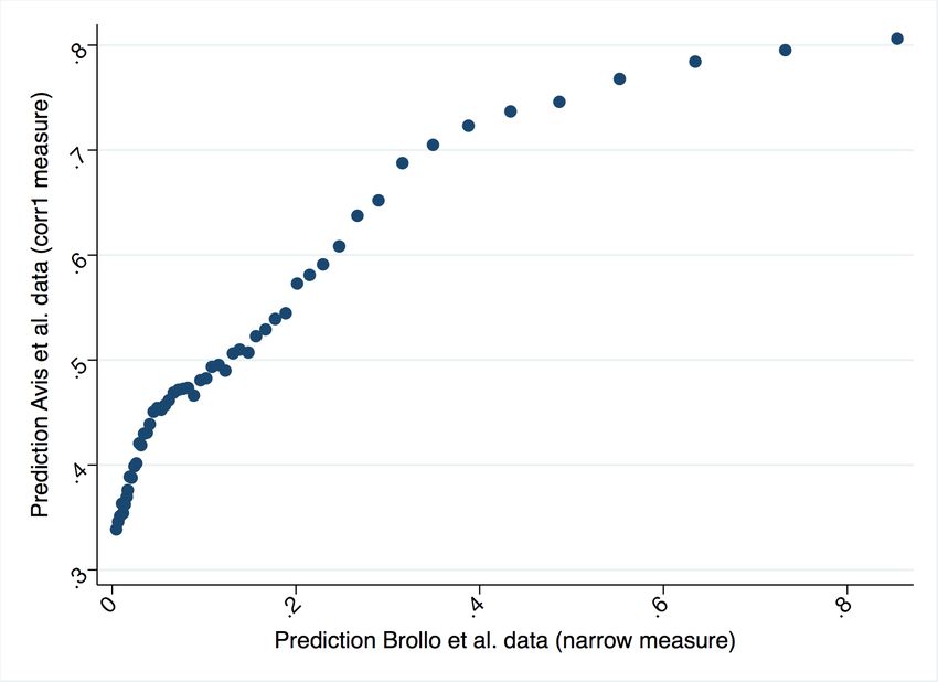
For robustness, we have access to an alternative set of corruption labels from Avis
et al. (2018). This measure is constructed using a slightly different approach to coding
the audit report documents. It is available for a different (but mostly overlapping) set
of audits. We find that the two measures are highly correlated (Appendix Figure A3).
In Appendix B, we will provide supplementary analysis using this alternative measure
of corruption.
5
In addition, they define a measure of broad corruption, which also includes inconsistencies that could
be linked to government mismanagement, but not intentional misuse. This concept of corruption is less
useful because it is so widespread: 76% of audited municipalities have broad corruption.
92.3. Linked Dataset
We join the corruption labels, which are defined at the municipality-term level, with
the local budget factors, which are defined at the municipality-year level. The resulting
dataset is at the municipality-year level. We then add data on local demographics, on
intergovernment transfers, and political party control. Specifically, we add demographics
from the 2000 Brazilian Census, including mean income, share of population employed,
sector of occupation (agriculture, industry, commerce, transportation, services and pub-
lic administration), share with college education, poverty rate, and Gini Coefficient of
income. Federal-to-municipal revenue transfers data come from the Brazilian National
Treasury (Tesouro Nacional ). Population data from the Brazilian Institute of Geog-
raphy and Statistics (IBGE). Finally, we collected information about the mayor party
affiliations in the 2000, 2004, and 2008 elections. Summary statistics on these variables
are reported in Table 1.
3. Predicting Corruption from Budget Data
Our goal is to take the information in the municipal budget and learn a prediction
function to provide a probability that a given municipality is fiscally corrupt. To that
end, this section outlines how we build our dataset and machine learning model to form
those predictions. We evaluate and interpret the predictive model, and then apply it to
all municipalities in Brazil for use in the subsequent analysis.
3.1. Corruption Prediction Dataset
Our data consists of budget predictors and corruption labels. For the budget features
X, we don’t undertake any additional pre-processing steps besides imputing missing
values with the mean value for the associated variable.6 The resulting matrix X of budget
factors has 897 columns, corresponding to the budget fields, and rows corresponding to
each municipality and year.
The corruption label Y ∈ {0, 1}, defined at the municipality-year level during terms
subject to audit, equals one for years where an audit found narrow corruption, and equals
zero for years when the audit did not find narrow corruption. For the machine learning
part, any municipality-terms that were not audited have to be excluded because we do
6
We got similar results when experimenting with additional pre-processing steps, including adding
missing indicator variables, (standardizing variables, or transforming variables as per capita.
10not have any labels. When municipalities were randomly audited more than once, we
exclude the second audit from the machine learning dataset.
3.2. Machine Learning Approach
We face a binary classification task. We want to learn a conditional expectation func-
tion Y (X) that provides a predicted probability that a municipality is corrupt based on
the publicly observed budget features. Economists are already familiar with logit or
probit (for example) in this setting. But these classical statistical models do not extrap-
olate well to new datasets because they tend to over-fit the training sample (e.g. Hastie
et al., 2009). The contribution of machine learning tools, now becoming widespread
in economics (e.g. Belloni et al., 2014; Mullainathan and Spiess, 2017; Athey, 2018), is
to address the over-fitting problem and provide robust out-of-sample prediction with
high-dimensional datasets.
Researchers and policymakers now have access to a variety of machine learning tools
for solving binary classification tasks. For example, one of the baseline models that we
will use below is penalized logistic regression. This model is very similar to the binary
logit, which learns a set of linear coefficients on X, sums them, and puts them through a
sigmoid transformation to obtain a probability for Y between zero and one. What is new
is a penalty term, which adds an additional cost to the training objective that penalizes
larger coefficients. The penalty addresses overfitting and helps the model predict better
in held-out test set data. During the training process the strength of the penalty is
calibrated in a process called cross-validation, where the training data is split up and
the out-of-sample performance of different penalties is evaluated. Then the best model
is taken to the unseen test set for a clean evaluation and for any downstream tasks.
A state-of-the-art model for binary classification using high-dimensional tabular datasets
is gradient boosted trees (Friedman, 2001; Hastie et al., 2009).7 Gradient boosting mod-
els consist of an ensemble of decision trees that “vote” on the predicted outcome. Each
decision tree iteratively selects informative variables (e.g., property taxes), splits on a
value of that variable (e.g., x > 100), branches off for additional splitting, and so on,
until reaching a terminal node and an associated prediction (Ŷ = 0 or Ŷ = 1). With
gradient boosting, additional layers of trees are gradually added during the training pro-
cess to fit residuals and fix errors in the initial layers. This iterative growth approach
7
This is the same algorithm used by Kleinberg et al. (2018) in predicting criminal recidivism.
11tends to perform better than other ensemble methods, such as random forests, which
grow trees in parallel.
More specifically, we train a gradient boosted classifier using the implementation
from the python package XGBoost (Chen and Guestrin, 2016). Feurer et al. (2018)
systematically compared XGBoost to many other classifiers, including a sophisticated
automated ML system, and found that XGBoost consistently performed best on our type
of machine learning task. We used cross validation grid search to tune hyperparame-
ters, which include the learning rate, L1 and L2 regularization penalties on the learned
parameter weights, the max depth of the constituent decision trees, and an additional
regularization constraint specifying a minimum threshold for the size of decision tree
terminal nodes. Appendix Table A2 shows the selected values for these hyperparameters
across each of five different training folds.
In the next subsection on model performance, we compare XGBoost to a number of
baselines. First, as the weakest baseline, we guess the modal category (not corrupt). Sec-
ond, we train ordinary least squares (OLS), or non-penalized linear regression, dropping
multi-collinear predictors. Third, LASSO, perhaps the most familiar machine learning
model to economists (e.g Belloni et al., 2014), is a linear regression model but adds
an L1 penalty that penalizes larger coefficients and outputs a sparse model. For both
OLS and LASSO, the predicted probabilities for Y might be below zero or above one,
but a decision threshold of 0.5 is used for assigning a predicted label. Finally, as the
strongest alternative baseline, we use penalized logistic regression, a linear classifier with
a sigmoid transformation and elastic net penalty (that is, both a LASSO (L1) and a
ridge (L2) penalty). For LASSO and Logistic, the penalty is selected by cross-validation
grid search in the training set. All three of these linear baselines are implemented using
the stochastic gradient descent learners from the python package scikit-learn (Pedregosa
et al., 2011).
We train and evaluate models using nested cross-validation, which works as follows:
First, we randomly split the sample of audited municipalities into five different sets.
Next, we train five separate models using each time four different subsets (80% of the
sample) and take the tuned models to get performance metrics in the test set (the
remaining 20 % of the sample). Each time, we tune the hyperparameters in the training
set using five-fold cross-validation. In each fold, early stopping is used (with patience of
ten training epochs) to stop training when the model begins to over-fit the training set.
Appendix Table A2 shows that the resulting forests consist of between 46 and 72 trees,
12Table 2: Machine Learning Metrics for Predicting Corruption
OLS Lasso Logistic XGBoost
(1) (2) (3) (4)
Accuracy 0.476 0.474 0.560 0.723
(0.022) (0.022) (0.022) (0.012)
AUC-ROC 0.487 0.507 0.568 0.777
(0.016) (0.012) (0.016) (0.013)
F1 0.685 0.538 0.545 0.632
(0.031) (0.050) (0.054) (0.018)
Notes: Columns report the mean and standard error (in paren-
theses) for the indicated performance metrics (by row) across
the five model runs, produced using separate training-set folds.
Columns indicate the machine learning model used.
each with up to 10 variable splits before a terminal node.
The nested approach provides five sets of predictions for each model. In the model
evaluation section, we have five sets of test-set evaluation metrics. We report the mean
and standard error across these five models. In the downstream tasks, and in particular
the policy simulation, we will use the multiple predictions to assess the importance of
sampling variability in the predictions.
3.3. Model Performance
We evaluate our set of models by their scores on a set of standard classification
metrics in the held-out test data. These metrics, reported by row in Table 2 Panel A,
describe how well a model trained on budget accounts can replicate the auditing agency’s
judgments about fiscal corruption. First, the most straightforward metric is accuracy,
which gives the proportion of test-set observations for which the machine-predicted la-
bel matches the true label. A naive guessing model that chooses the modal category
(not corrupt) would obtain accuracy = 0.58. Second, we report AUC-ROC (area under
the receiver operator characteristic curve), another standard metric in binary classifi-
cation. AUC-ROC, which takes values between 0.5 (random guessing) and 1.0 (perfect
accuracy), can be interpreted as the probability that a randomly sampled corrupt mu-
nicipality is ranked more highly by predicted probability of corruption than a randomly
sampled non-corrupt municipality. Third, we report F1 for the corrupt class, defined as
the harmonic mean of precision (proportion true corrupt within the set predicted cor-
13rupt) and recall (proportion predicted corrupt within the set true corrupt). F1, ranging
from 0.0 (guessing the modal category) and 1.0 (perfect accuracy for the corrupt class),
penalizes both false positives and false negatives.
Across the columns of Table 2, we compare the predictive performance of our preferred
model, XGBoost, to a number of other baselines. In each table cell, we report the average
test-set performance metric across the five cross-validated model runs, with the standard
error of the mean in parentheses. In the text, we report the minimum and maximum
metric values across the folds.
In the rightmost Column 4, we report the metrics from our preferred model, the
gradient boosting classifier. The average test set accuracy for the predictions across five
nested folds is 0.723, with the minimum accuracy being 0.692 and the maximum 0.755.
For AUC-ROC, the average is 0.777 (with min = 0.743 and max = 0.809), while for F1,
the average is 0.632 (min = 0.584, max = 0.675). To help contextualize these numbers,
the model is similar in its performance to the one used by Kleinberg et al. (2018) to
predict criminal recidivism by defendants in pre-trial bail proceedings.8 For comparison,
we form predictions using OLS (Column 1), LASSO (Column 2), and Logistic Regression
(Column 3). The predictions provided by OLS or LASSO are barely better than random
guessing. Logistic regression is somewhat better but still much worse than XGBoost.
This difference in performance suggests a nonlinear, interactional relationship among the
predictors that the tree ensemble is better able to learn.
Appendices A and B report additional evaluations of the prediction task. First, to
help visualize the distribution of predictions, Appendix Table A3 shows the confusion
matrices for the test-set predictions. For XGBoost, we can see good precision and recall
across categories. The confusion matrices for OLS, LASSO, and logistic regression show
that the linear models tend to produce many false positives (not-corrupt municipalities
are often labeled as corrupt).
Second, we focus on the municipalities that have been audited twice and see if our
prediction model can reproduce within-municipality changes in corruption over time.
To that end, we regress the change in true corruption against the change in predicted
corruption, adjusting for audit year fixed effects and demographic characteristics. Ap-
pendix Figure A1 shows that there is a significant positive effect in this regression. This
within-municipality validation is important for the usefulness of our measure in empirical
8
Kleinberg et al. (2018) report an AUC-ROC of 0.707 for their best-performing model.
14tasks, where one would like to be able to examine changes in corruption over time.
Third, in Appendix Table A10 we report performance metrics with an alternative
sampling approach and with an alternative corruption label. In Columns 1-3, we apply
random splits between training and test set by municipality, instead of by municipality-
year, which allows us to compare the model performance using budget factors, fixed
demographic factors, or both. The alternative sampling approach obtains comparable
performance to our baseline model and shows that a model trained using just demo-
graphic information is less accurate than a model using budget information. In Columns
4-7, we show the model performance for the alternative corruption label from Avis et al.
(2018). We see that our XGBoost model is even more accurate in predicting the alter-
native label (AUC-ROC = 0.903, s.e. = 0.009).
3.4. Interpreting the Predictions
Gradient boosted machines, like all ensembles and other sophisticated machine learn-
ing algorithms, are black boxes. At the end of model training, we have a dense forest
of decision trees. With 797 variable being input into those trees, and hundreds of splits
within the forest, it is difficult to tell how the model is making its predictions. In this
subsection we use model explanation methods to better understand how the model works.
The previous applied machine learning literature has discovered an advantage of
gradient boosted machines that compensates for their basic lack of interpretability (e.g.
Hastie et al., 2009). One can rank the input variables by their feature importance,
computed as the number of times the model “uses” that variable in the sense that one
of the constituent decision trees splits on it. Note that these features could be either
positively or negatively correlated with the predicted corruption. The ranking is more
informative than seeing which predictors are correlated with corruption, because they
could be important through a non-linear relation, or through interactions with other
variables. Moreover, the important features can be seen as pivotal in the sense that they
are the most useful variables for predicting the outcome, even among clusters of highly
collinear predictors.
Here we use the feature importance ranking to get some insight into how our cor-
ruption detection model makes its predictions. After model training, we have feature
importance scores for each of the five cross-validated models. We average the scores
across folds and then rank the most important features.
From the feature importance scores, we learn immediately that our dataset contains
15Table 3: Most important budget features for Corruption Prediction
N. Category Macro Category Weight
1 Tax on agricultural territorial property (ITR) (compartecipation) Revenue 103
2 Spending in agriculture Expenditure 103
3 Spending in transportation Expenditure 95
4 Tax on export of industrialized products (IPI) (compartecipation) Revenue 92
5 Budget Surplus/Deficit 84
6 Cash Assets 84
7 Tax on real estate transactions (ITB) Revenue 80
8 Taxes Revenue 79
9 Deposits Assets 76
10 Motor vehicle property tax (IPVA) (compartecipation) Revenue 74
11 Income Tax (IRRF) Revenue 73
12 Transfers for the health system Revenue 71
13 Civil servant per diems Expenditure 70
14 Spending for legislative procedure Expenditure 68
15 Revenue from assets Revenue 67
Notes: List of the most important features. Metrics rank the features (budget components) by how often they are
included in a decision tree contained in the ensemble classifier, averaged across the five training folds.
many noise predictors. Out of the 797 variables input to the ensemble, only 446 are used
at all and 351 are ignored by the ensemble across all five folds. Within the set of useful
variables, we show the 15 predictors with the highest feature importance scores in Table
3.
The most frequent categories identified as relevant to corruption are those related
to expenditures and taxes. On expenditures, we see corruption-related spending for
agriculture (2), public services in transportation (3), coherently with Hessami (2014),
and legislative actions of local government (14). Other specific signals come from the
arbitrary use of public funds in categories that are perhaps more difficult to monitor, for
instance, civil servant per diems (13). Many variables are also included on the taxes side
(Liu and Mikesell, 2019), with the model especially attending to income tax (11) and
different types of property taxes. These include property taxes on agricultural land (1),
on motor vehicles (10), and on transfers of real estate ownership (7). The latter variable
is related to the construction sector, traditionally associated to corruption (Kyriacou
et al., 2015). Some of these categories refer to national tax revenues that are transferred
to municipalities, as in the case of taxes from export of industrialized products (4). Other
non-tax revenues that made it to the list include transfers from other government levels
to fund the public health system (12), as studied in Machoski and de Araujo (2020), and
revenues generated from municipal assets (e.g., real estate) (15). In terms of assets, we
find liquid assets, such as cash (6) and the more general classification of deposits (9).
16Figure 1: Model-Predicted Feature Importance and Mentions in Audit Report Texts
Notes: Binscatter diagram for frequency that a budget feature appears in the
municipal audit reports (vertical axis) against binned feature importance weights
for each feature (horizontal axis). Pearson’s correlation is 0.13. The regression
coefficient is 0.097 with p = .09 (robust standard errors).
Finally, the model attends to the presence of a budget deficit/surplus, in line with Liu
et al. (2017), showing the link between public corruption and debt.
While the model’s identification of these important budget features is consistent with
some work from the literature, listing these examples is somewhat ad hoc. To see whether
the feature importance scores can validate our model more quantitatively, we would like
to know whether these pivotal features were actually identified as related to corruption
by the auditors in Brazil. To do that, we look for mentions of these items in the best
available place – the text of the published audit reports.
To this end, we downloaded the full library of audit reports for our time period as
PDF files from the agency web site. The PDFs were in machine-readable Portuguese
and therefore straightforward to extract as plain text. We performed mild cleaning the
language, namely removing punctuation and capitalization. The same was done for our
list of budget accounting variable names. Finally, we counted the total mentions of each
budget feature in the corpus of reports.
We then produced a dataset at the prediction variable level, containing the percentile
17rank in the model feature importance score and the percentile rank in the audit-report
mention count. Figure 1 plots the audit mention percentiles against the feature impor-
tance percentiles. We see a clear positive relationship that is statistically significant in
a univariate regression (p = .09). Our classifier, trained on the budget accounts with
just corruption labels, identifies as important the same budget features that tend to be
mentioned in the audit report documents. These validation results support the view
that our measure captures activities that are indeed related to corruption.
3.5. Measuring Corruption in Non-Audited Municipalities
An essential contribution of our approach is to measure corruption for all Brazilian
municipalities and all years from 2001 to 2012. Using the trained models, we form five
predicted corruption probabilities for all observations based on the budget data. In
Figure 2 we provide a visualization of the difference between the sample of only audited
municipalities (Panel a) and the sample of municipalities that we can analyze when
using our predicted measure of corruption (Panel b). The map illustrates quite clearly
the additional information produced by the machine learning method. With the machine
predictions, we can then analyze corruption in municipalities (and years) regardless of
whether they have been audited.
4. Empirical Applications
This section replicates and extends existing evidence from the literature on corruption
in Brazil. This exercise has two purposes. On the one hand, it provides checks on the
internal validity of our synthetic measure of corruption – that is, we can check whether
it responds to causal treatments the same way as auditor-measured corruption. On
the other hand, we extend previous results by taking advantage of the larger sample of
municipalities and the time variation of our corruption measure.
4.1. Revenue Shocks and Corruption
As a first analysis, we use the new synthetic measure of corruption to analyze the
effect of revenue shocks on corruption, replicating and extending the findings by Brollo
et al. (2013). This paper studies whether a windfall of public revenues can lead to
an increase in rent-seeking by the public administration (as measured by a subsequent
surge in corruption). They estimate the impact of federal transfers on the occurrence of
corruption as detected by the random audits.
18Figure 2: The Geography of (Predicted) Corruption
(a) Actual Corruption
(b) Predicted Corruption
Notes: Actual (Panel a) and predicted (Panel b) corruption by municipality, using
budgets from 2004. A municipality is predicted to be corrupted if mean prediction
is >0.5.
19Brazilian municipalities receive transfers from the states and from the federal govern-
ment. Federal transfers are the largest single source of municipal revenues (around 40%
of the total budget). The amount transferred through this FPM program (Fundo de
Participação dos Municipios) depends on exogenous population thresholds, where mu-
nicipalities in the same state and in a given population bracket receive the same amount
of resources.9
More precisely, the amount of revenues received by municipality i in state k follows
the allocation mechanism:
F P Mk λi
F P Mik = P
i∈k λi
where F P Mk is the total amount allocated in state k and λi is the municipality-specific
coefficient, as shown in Table A4. Due to imperfect compliance, however, the statuto-
rily prescribed transfers do not perfectly determine the amounts actually transferred.10
Thus, Brollo et al. (2013) use a fuzzy regression discontinuity design methodology, in-
strumenting actual transfers (τi ) with theoretical transfers (τ̂i ).
Formally, we have the first stage
τi = g(Pi ) + ατ τˆi + δt + γp + ui (1)
and reduced form
yi = g(Pi ) + αy τˆi + δt + γp + ηi (2)
where yi is corruption, g(·) is a high order polynomial in Pi (the population of city
i), δt contains term fixed effects, γp contains state fixed effects, and ui and ηi are the
error terms. The coefficients ατ and αy capture the effects of theoretical transfers on
actual transfers and (predicted) corruption, respectively. For the two-stage-least squares
analysis, we estimate the second stage
yi = g(Pi ) + βy τi + δt + γp + i (3)
9
Appendix Table A4 shows these coefficients and the corresponding population brackets: Following
Brollo et al. (2013), we focus on the initial seven brackets and restrict the sample to cities with a
population below 50,940. Furthermore, we follow the approach of Brollo et al. (2013) and restrict the
sample, for the sake of symmetry, to municipalities from 3,396 below the first threshold to 6,792 above
the seventh threshold. This sample represents about 90 percent of Brazilian municipalities.
10
This imperfect compliance is due to many factors (e.g. municipalities splitting, manipulation in
population figures). See Brollo et al. (2013).
20where theoretical transfers τˆi are used as an instrument for actual transfers τi and all
other terms are defined as above. The coefficient βy captures the causal effect of ac-
tual transfers on (predicted) corruption. For inference, standard errors are clustered by
municipality.11
Our data cover the two mayoral terms, January 2001–December 2004 and January
2005–December 2008. While Brollo et al. (2013) focus only on municipalities that re-
ceived an audit, our dataset allows us to analyze a larger and more representative sample
of cities. Therefore, our exercise is also providing a test for the external validity of their
results.12 Appendix table A5 shows the descriptive statistics by population bracket.
Brazilian municipalities in our sample receive, on average, $3.3M BRL (about $610K
USD), while theoretical transfers are somewhat higher at $3.7M BRL (about $680K
USD). The average level of (predicted) corruption is around 0.5 and its level does not
change significantly as we move to larger cities.
Table 4 reports the results for the regression analysis. Panel A shows the estimates
of the first stage, Equation (1), Panel B shows the reduced-form effects, Equation (2),
while Panel C shows the the corresponding two-stage-least-squares estimates. For each
panel, we provide the results when including: cities that have received an audit (column
1) similarly to Brollo et al. (2013), all cities (column 2), and cities that have never been
audited (column 3).
We find a strong first-stage effect, showing that theoretical transfers positively affect
actual transfers, and this is true for all samples considered. In addition, we find positive
and significant coefficients when estimating the reduced-form as well as the two-stage-
least-squares results. Varying the sample of interest does not significantly alter the size of
coefficient and the level of precision is stable. Notably, the magnitude of the standardized
reduced-form coefficient is about four-fifths the size of that estimated by Brollo et al.
(2013), and our 95% confidence interval contains the original coefficient. Thus even the
magnitudes of empirical estimates using machine-learning-measured corruption seem to
be comparable to using auditor-measured corruption.
To test the robustness of these empirical results, we conducted a series of checks.
First, we replicate the main analysis on four random samples of 1,115 municipalities, the
11
See Brollo et al. (2013) for a detailed discussion and testing of the econometric assumptions in this
setting.
12
For the sake of brevity we only replicate the analysis on the overall effect, omitting the threshold-
specific analysis.
21Table 4: Replication Analysis: Effect of Revenue Shocks on Corruption
Audited cities All cities Non-audited cities
(1) (2) (3)
Panel A. First Stage
Theoretical transfers 0.6805*** 0.6909*** 0.6996***
(0.0205) (0.0233) (0.0230)
Panel B. Reduced Form
Theoretical transfers 0.0040*** 0.0041*** 0.0040***
(0.0009) (0.0003) (0.0003)
Panel C. 2SLS
Actual transfers 0.0058*** 0.0059*** 0.0057***
(0.0013) (0.0005) (0.0005)
N. Observations 1115 5808 4693
Notes: Effects of FPM transfers on (predicted) corruption measures. Panel A reports the
estimates of the first-stage analysis, the dependent variable is actual transfers. Panel B
reports the estimates of reduced form analysis, the dependent variable is predicted cor-
ruption. Panel C reports the estimates of the 2sls estimates, the dependent variable is
predicted corruption and actual transfers is instrumented with theoretical transfers. Col-
umn headings indicate the sample of municipalities included. All regressions controls for
a third-order polynomial in normalized population size, term dummies, and macro-region
dummies. Robust standard errors clustered at the municipal level are in parentheses: *
p < 0.10, ** p < 0.05, *** p < 0.01.
22sample size of the original analysis by Brollo et al. (2013) (Appendix Table A6). The co-
efficients show some variation, but they are always positive and statistically significant.
Second, we show that the instrument is not correlated with the error of the prediction
model, defined as the difference between the true corruption level and the predicted one
(p-value=0.212). This null is helpful because it suggests that the model errors are not
responding to the instrument. That is, the correlated factors besides corruption that
are contributing to our prediction are not affected directly by revenue transfer shocks.
Thus, using our model predictions as the outcome will still satisfy the exclusion restric-
tion. Third, we show in Appendix Table A7 Column 1 that there is no revenue-shock
effect on a corruption prediction formed with a model trained on municipal demographic
characteristics (similar to Collonelli et al’s). This placebo test is reassuring because the
model trained on demographics does not contain budget information, and means that
our model is not forming corruption predictions based on spurious correlations with de-
mographics. Fourth, we formed predictions from our baseline model while permuting
randomly the FPM transfer variable, which could be mechanically shifted by the rev-
enue shocks instrument. The effect of revenue shocks is the same (Appendix Table A7
Column 2).
Overall, this replication exercise provides helpful validation for the use of our pre-
dicted measure of corruption in contexts where audits provide insufficient data. In
addition, we provide additional evidence on the external validity of findings by Brollo
et al. (2013).
4.2. Effect of Audits on Corruption
The next empirical application uses our predicted measure of corruption to analyze
the effect of auditing on subsequent corruption in an event study framework. This
analysis complements Avis et al. (2018), who explore the same research question using
the set of Brazilian municipalities that were (by random draw) audited twice in a cross-
sectional setup. With our new measure of predicted corruption, we can overcome the
data limitations of Avis et al. and extend their results. First, because of the longitudinal
nature of our dataset, we can capture dynamic effects. Second, we can condition our
estimates on pre-audit levels of corruption. Third, our effects are identified by a relatively
23larger sample of municipalities that got audited only once (rather than twice).13
Using the annual corruption prediction yist in municipality i of state s at year t, we
take a standard event study approach and estimate the within-municipality effects of a
k
(randomly assigned) audit. Let Dist be a dummy variable for k years before and after
an audit. We estimate
5
X
k 0
yist = βk Dist + δi + λt + Wist φ + ist (4)
k=−3,k6=−1
where we have municipality fixed effects δi , year fixed effects λt and other controls Wist ,
which in particular includes dummy variables indicating periods distant from when the
audit took place. Because k 6= −1 (the year before the audit), the βk estimate the
dynamic effects relative to the year before the audit. The identifying assumption hinges
on randomness in the timing of selection into the audit program. We cluster standard
errors by state. The sample includes 1,479 municipalities that have received an audit in
the time period under analysis.
We graphically report estimates for Equation (4) in Figure 3 Panel (a), with the
numerical estimates reported in Appendix Table A8. We can see that already in the
year of the audit (k = 0), there is a sharp and statistically significant drop in predicted
corruption. This persists over the subsequent years but becomes weaker. Meanwhile,
as expected given the random assignment due to the lottery, there is no statistically
significant effect in the pre-announcement years.
Panel (b) reports event-study effects for the subsets of audits that find clear corrup-
tion (black points) and those that do not find corruption at all (grey points).14 These
trends look quite different. When corruption is discovered (black points), there is a much
larger negative effect ranging between -1.7% and -25.8%, which is sizeable if compared
with the magnitude of the treatment mean of 55.8%. The effect is persistent across sub-
sequent years. In contrast, when the audit does not find any corruption or irregularities
(grey points), there is no effect on corruption. Such effects could consist of an actual
13
Bobonis et al. (2016) study a similar research question in Puerto Rican municipalities. The authors
focus on (non random) audit of municipal accounts, finding that audits do not persistently reduce
corruption in that case.
14
The former group includes those cities in which the audits discovered a positive amount of corruption
(measured with the variable narrow corruption), while the latter group includes those municipalities in
which the audit did not find any type of corruption.
24You can also read