Additional carbon inputs to reach a 4 per 1000 objective in Europe: feasibility and projected impacts of climate change based on Century ...
←
→
Page content transcription
If your browser does not render page correctly, please read the page content below
Biogeosciences, 18, 3981–4004, 2021
https://doi.org/10.5194/bg-18-3981-2021
© Author(s) 2021. This work is distributed under
the Creative Commons Attribution 4.0 License.

Additional carbon inputs to reach a 4 per 1000 objective in Europe:
feasibility and projected impacts of climate change based on
Century simulations of long-term arable experiments
Elisa Bruni1 , Bertrand Guenet1,2 , Yuanyuan Huang3 , Hugues Clivot4,5 , Iñigo Virto6 , Roberta Farina7 ,
Thomas Kätterer8 , Philippe Ciais1 , Manuel Martin9 , and Claire Chenu10
1 Laboratoire des Sciences du Climat et de l’Environnement, LSCE/IPSL, CEA-CNRS-UVSQ, Université Paris-Saclay,
91191 Gif-sur-Yvette, France
2 LG-ENS (Laboratoire de géologie) – CNRS UMR 8538 – École normale supérieure, PSL University – IPSL,

75005 Paris, France
3 CSIRO Oceans and Atmosphere, Aspendale 3195, Australia
4 Université de Lorraine, INRAE, LAE, 68000 Colmar, France
5 Université de Reims Champagne Ardenne, INRAE, FARE, UMR A 614, 51097 Reims, France
6 Departamento de Ciencias. IS-FOOD, Universidad Pública de Navarra, 31009 Pamplona, Spain
7 CREA – Council for Agricultural Research and Economics, Research Centre for Agriculture and Environment,

00198 Rome, Italy
8 Swedish University of Agricultural Sciences, Department of Ecology, Box 7044, 75007 Uppsala, Sweden
9 INRA Orléans, InfoSolUnit, Orléans, France
10 Ecosys, INRA-AgroParisTech, Universiteì Paris-Saclay, Campus AgroParisTech, 78850 Thiverval-Grignon, France

Correspondence: Elisa Bruni (elisa.bruni@lsce.ipsl.fr)

Received: 25 December 2020 – Discussion started: 12 January 2021
Revised: 31 May 2021 – Accepted: 4 June 2021 – Published: 2 July 2021

Abstract. The 4 per 1000 initiative aims to maintain and in-       ditional C inputs from exogenous organic matter or changes
crease soil organic carbon (SOC) stocks for soil fertility, food   in crop rotations, and was able to reproduce the SOC stock
security, and climate change adaptation and mitigation. One        dynamics.
way to enhance SOC stocks is to increase carbon (C) inputs            We found that, on average among the selected ex-
to the soil.                                                       perimental sites, annual C inputs will have to increase
   In this study, we assessed the amount of organic C in-          by 43.15 ± 5.05 %, which is 0.66 ± 0.23 Mg C ha−1 yr−1
puts that are necessary to reach a target of SOC stocks in-        (mean ± standard error), with respect to the initial C inputs
crease by 4 ‰ yr−1 on average, for 30 years, at 14 long-term       in the control treatment. The simulated amount of C input
agricultural sites in Europe. We used the Century model to         required to reach the 4 ‰ SOC increase was lower than or
simulate SOC stocks and assessed the required level of addi-       similar to the amount of C input actually used in the majority
tional C inputs to reach the 4 per 1000 target at these sites.     of the additional C input treatments of the long-term experi-
Then, we analyzed how this would change under future sce-          ments. However, Century might be overestimating the effect
narios of temperature increase. Initial stocks were simulated      of additional C inputs on SOC stocks. At the experimental
assuming steady state. We compared modeled C inputs to             sites, we found that treatments with additional C inputs were
different treatments of additional C used on the experimental      increasing by 0.25 % on average. This means that the C in-
sites (exogenous organic matter addition and one treatment         puts required to reach the 4 per 1000 target might actually
with different crop rotations). The model was calibrated to fit    be much higher. Furthermore, we estimated that annual C in-
the control plots, i.e. conventional management without ad-        puts will have to increase even more due to climate warming,

Published by Copernicus Publications on behalf of the European Geosciences Union.
3982                                    E. Bruni et al.: Additional carbon inputs to reach a 4 per 1000 objective in Europe

that is 54 % more and 120 % more for a 1 and 5 ◦ C warming,        ity (Lal 2008), indirectly enhancing agricultural productivity
respectively. We showed that modeled C inputs required to          and food security.
reach the target depended linearly on the initial SOC stocks,         SOC stocks are a function of C inputs and C outputs. To
raising concern on the feasibility of the 4 per 1000 objective     increase SOC stocks, one can either increase C inputs to the
in soils with a higher potential contribution to C sequestra-      soil (i.e. adding plant material or organic fertilizers) or re-
tion, that is soils with high SOC stocks. Our work highlights      duce C outputs resulting from mineralization and, in some
the challenge of increasing SOC stocks at a large scale and        cases, soil erosion. Increasing SOC stocks can be achieved
in a future with a warmer climate.                                 via agricultural practices such as retention of crop residue
                                                                   and organic amendments to the soil, cover cropping, diversi-
                                                                   fied rotations and agroforestry systems (Chenu et al., 2019;
                                                                   Powlson et al., 2011). However, some of these practices only
                                                                   lead to local carbon storage at the field scale, rather than a
1   Introduction                                                   net carbon sequestration from the atmosphere at larger scales
                                                                   (Chenu et al., 2019).
Increasing organic carbon (C) stocks in agricultural soils            Assessing the evolution of SOC stocks over time is im-
is beneficial for soil fertility and crop production and for       portant to correctly estimate the potential of SOC storage
climate change adaptation and mitigation. This considera-          in agricultural soils and evaluate management practices in
tion was at the basis of the 4 per 1000 (4p1000) initia-           terms of both SOC stock increase and sequestration potential.
tive, proposed by the French government during the 21st            The dynamics of SOC stocks can be either measured in agri-
Conference of the Parties (COP21) on climate change. The           cultural soils through long-term experiments (LTEs) and soil
4p1000 initiative aims to promote agricultural practices that      monitoring networks or estimated via biogeochemical mod-
enable the conservation of organic carbon in the soil (https:      els (Campbell and Paustian, 2015; Manzoni and Porporato,
//www.4p1000.org, last access: 25 June 2021). Because soil         2009). Combining measurements of SOC with models pro-
organic carbon (SOC) stocks are 2 to 3 times higher than           vides a wider applicability of the information collected in
those in the atmosphere, even a small increase in the SOC          field trials, as it allows SOC stocks and their future trends
pool can translate into significant changes in the atmospheric     to be estimated. However, validity of models in the studied
pool (Minasny et al., 2017). To demonstrate the importance         areas has to be assessed, and models need to be initialized.
of SOC, the initiative took as an example the fact that in-        This means that the initial status of SOC has to be set, either
creasing global SOC stocks up to 0.4 m depth by 4p1000             for lack of data on total initial stocks or to determine the al-
(0.4 %) per year of their initial value could offset the net an-   location of C among the model’s compartments that cannot
nual carbon dioxide (CO2 ) anthropogenic emissions to the          be measured. This is commonly accomplished by assuming
atmosphere (Soussana, 2017). While increasing SOC stocks           that SOC is at equilibrium at the beginning of the experiment
by 4p1000 annually is not a normative target of the initiative,    (Luo et al., 2017; Xia et al., 2012).
this value can be taken as a reference to which current situ-         The feasibility and applicability of a 4 ‰ increase target
ations and alternative strategies are compared (e.g., Pellerin     depend on biotechnical and socio-economic factors. As we
et al., 2019).                                                     mentioned earlier, a number of practices are known to in-
   Strategies of conservation and expansion of existing SOC        crease SOC stocks in agricultural systems. However, it is still
pools may be necessary but are not sufficient to mitigate cli-     debated whether they will be sufficient to reach the 4p1000
mate change (Paustian et al., 2016). In this sense, increas-       objective. Minasny et al. (2017) described opportunities and
ing SOC stocks cannot be regarded as a dispensation to con-        limitations of a 4 ‰ SOC increase in 20 regions across the
tinue business as usual, but rather as a wedge of negative         world. Several authors (e.g., Baveye et al., 2018; van Groeni-
greenhouse gas (GHG) emissions (Wollenberg et al., 2016),          gen et al., 2017; VandenBygaart, 2018) argued that some of
as well as a strategy for improving most soils’ resilience to      the examples described in Minasny et al. (2017) were not
changes in the climate.                                            representative of wide-scale agriculture and suggested that a
   The potential to increase SOC stocks is particularly rel-       4 ‰ rate is not attainable in many practical situations (Poul-
evant in cropped soils, where the depletion of organic mat-        ton et al., 2018). Implementing new agricultural practices
ter with respect to the original non-cultivated situation has      that allow the maintenance and increase in SOC stocks might
been demonstrated (Clivot et al., 2019; Goidts and van Wese-       require structural land management changes that not all farm-
mael, 2007; Meersmans et al., 2011; Saffih-Hdadi and Mary,         ers will be willing to adopt. Incentivizing and sustaining vir-
2008; Sanderman et al., 2017; Zinn et al., 2005) and where         tuous practices to increase SOC stocks should be a strategy
straightforward management practices can be implemented            for policymakers to overcome socio-economic barriers (e.g.,
to promote the conservation or increment of SOC (Chenu             Lal, 2018; Soussana, 2017), and in order to do that, they
et al., 2019; Guenet et al., 2020; Paustian et al., 2016). More-   need to be correctly informed. Recent works have assessed
over, increasing the organic C content in agricultural soils is    the biotechnical limitations of a SOC increase, studying the
known to improve their fertility and water retention capac-        required and available biomass to reach a 4p1000 target in

Biogeosciences, 18, 3981–4004, 2021                                                   https://doi.org/10.5194/bg-18-3981-2021
E. Bruni et al.: Additional carbon inputs to reach a 4 per 1000 objective in Europe                                          3983

European soils (Wiesmeier et al., 2016; Martin et al., 2021;      turnip), oilseed crops (sunflower and oilseed rapeseed) and
Riggers et al., 2021).                                            cover crops (mustard and rapeseed), and one rotation in-
   Our work was set up in this context with the objectives to     cluded tomatoes. Straw residue was systematically exported
(1) estimate the amount of C inputs needed to increase SOC        except at French sites, where residue was sometimes incor-
stocks by 4 ‰ yr−1 , (2) investigate whether this amount is       porated into the soil as accounted for in the C input calcula-
attainable with currently implemented soil practices (i.e. or-    tions. All LTEs were under conventional tillage, which was
ganic amendments and different crop rotations) and (3) study      performed with a tractor, except in the case of Ultuna, where
how the required C inputs are going to evolve in a future         it was performed manually. All experiments were rainfed, ex-
driven by climate change. We used the biogeochemistry SOC         cept for Foggia, where tomatoes were irrigated in summer.
model Century, which is one of the most widely used and val-      The French sites Champ Noël 3, Crécom 3 PRO, La Jaillière
idated models (Smith et al., 1997a), to simulate SOC stocks       2 PRO, Le Rheu 1 and Trévarez received optimal amounts of
in 14 different agricultural LTEs around Europe. We set the       mineral fertilizers both in the control plot and in the different
target of SOC stock increase to 4 ‰ yr−1 for 30 years, rela-      organic matter treatments. All other experiments did not re-
tive to the initial stocks in the reference treatments. With an   ceive any mineral fertilization. All control plots, apart from
inverse modeling approach, we estimated the amount of ad-         Arazuri, had decreasing SOC stock trends (SOC approxi-
ditional C inputs required to reach a 4p1000 target at these      mated with a linear regression: SOC = m · t + SOC0 , with
                                                                                               m
sites. Finally, we evaluated the dependency of the required       average relative change: SOC   0
                                                                                                   · 100 = −0.76 %, R 2 = 0.58).
additional C inputs on different scenarios of increased tem-      Over the 46 treatments of additional C input, 18 exhibited
perature.                                                         increasing SOC stocks at a higher rate than 4 ‰ yr−1 on av-
                                                                  erage over the experiment length (Table 1). Six treatments
                                                                  had increasing SOC stocks, but at a lower ratio than 4p1000.
2     Materials and methods                                       The other 22 treatments with additional C inputs had decreas-
                                                                  ing SOC stocks (Mg C ha−1 ). However, the decreasing trend
2.1    Experimental sites                                         was, in these cases, lower than the decreasing trend in the
                                                                  respective control plot, in the majority of the treatments.
We compiled data from 14 LTEs in arable cropping systems
across Europe (Fig. 1), where a total of 46 treatments with       2.1.1   Climate forcing
increased C inputs to the soil were performed, and one con-
trol plot in each experiment was implemented (Table 1). The       Mean temperature of the sites ranged from a minimum of
experiments lasted between 11 and 53 years (median value          5.7 ◦ C to a maximum of 15.5 ◦ C, while mean soil humid-
of 16 years) in the period from 1956 to 2018. Most of the ex-     ity to approximately 20 cm depth ranged between 20.2 and
periments had at least three replicates, except for the Italian   24.6 kgH2 O m−2
                                                                                soil in the dataset (Table 2). When available, ob-
site Foggia, the French site Champ Noël 3 and the British site    served daily air temperature was used as an approximation
Broadbalk, where no replicates were available. We selected        of soil temperature. Otherwise, the land–atmosphere model
experiments where dry matter (DM) yields and SOC had              ORCHIDEE was used to simulate soil surface temperature
been measured at several dates. C inputs at all sites, except     and soil humidity at the site scale (Krinner et al., 2005).
for control plots and all plots in Foggia, included exogenous     ORCHIDEE simulations were run over each site using a 3-
organic matter (EOM) addition, e.g., animal manure, house-        hourly global climate dataset at 0.5◦ (GSWP3 http://hydro.
hold waste, sewage sludge or compost additions. In Foggia,        iis.u-tokyo.ac.jp/GSWP3/, last access: 1 September 2020).
different rotations without organic matter addition were stud-    Plant cover was set to C3 plant functional type (PFT) for agri-
ied and compared to a wheat-only treatment, considered the        culture.
control plot. The annual C inputs to the soil were substan-
                                                                  2.1.2   Soil characteristics
tially higher in the rotations compared to the control. More
information on crop rotations and C inputs for each treatment     The sampling depth of the experiments varied between 20
can be found in Table 1.                                          and 30 cm. SOC stocks were measured in three to four repli-
   Cropping systems in the 60 treatments (14 control plots        cates, apart from the Foggia and Champ Noël 3 experiments,
and 46 additional C input treatments) were mainly cereal-         where no replicates were available, and Broadbalk. In this
dominated rotations (wheat, maize, barley and oat). In partic-    experiment, SOC was measured in each plot using a semi-
ular, four were cereal monocultures (silage maize in Champ        cylindrical auger where 10–20 cores were taken from across
Noël 3, Le Rheu 1 and Le Rheu 2 and winter wheat in               the plot and bulked together (more details can be found on the
Broadbalk), and four sites had rotations of different cere-       e-RA website1 ). The clay content ranged from 10 % (Jeu-les-
als (winter wheat and silage or grain maize in Crécom 3           Bois) to 41 % (Foggia). Soil pH varied from a minimum of
PRO, Feucherolles, La Jaillière 2 PRO and Avrillé). The
other sites rotated cereal crops with legumes (chickpea, pea)        1 http://www.era.rothamsted.ac.uk, last access: 20 Febru-
and/or root crops (fodder beet, fodder rapeseed and Swedish       ary 2020.

https://doi.org/10.5194/bg-18-3981-2021                                                  Biogeosciences, 18, 3981–4004, 2021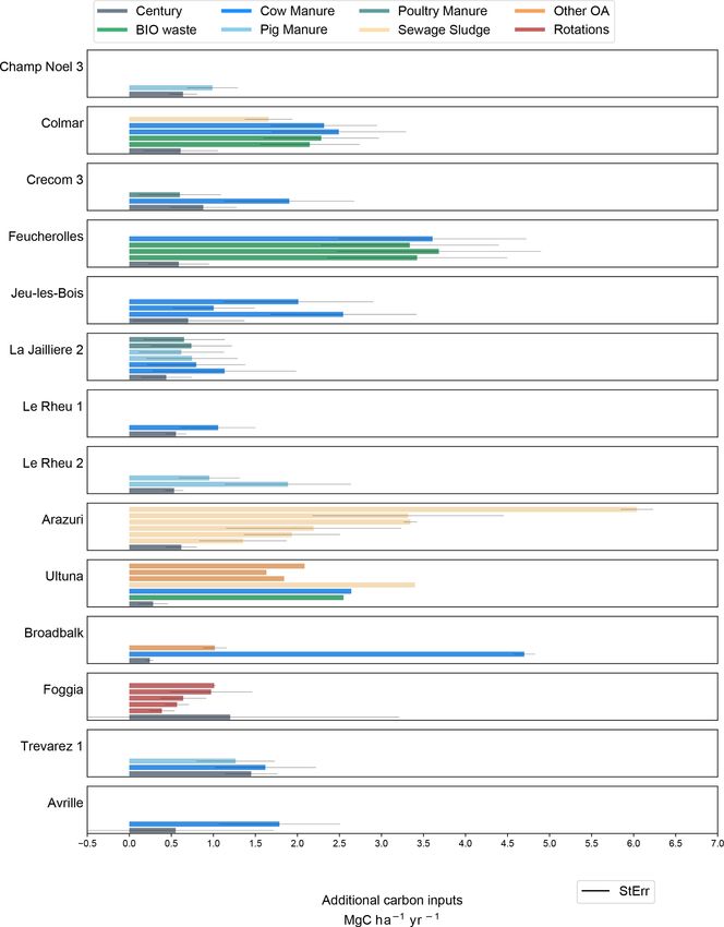
3984 E. Bruni et al.: Additional carbon inputs to reach a 4 per 1000 objective in Europe
Table 1. Summary of the agricultural experiments included in the study: crop rotations grown at site, amount of carbon inputs
(Mg C ha−1 yr−1 ) estimated from crop yields as in Bolinder et al. (2007), type of treatments, amount of additional organic carbon from
organic treatments (Mg C ha−1 yr−1 ) and mean annual SOC stock variation (%).
Site ID treatment Rotationsa Carbon inputs from Treatment type Additional carbon inputs SOC annual
crop rotations from organic treatments variation
Mg C ha−1 yr−1 Mg C ha−1 yr−1 %
Champ Noël 3 Minb sM 1.29 Reference + N b 0 −0.92
(CHNO3) LP Silage maize 1.49 Pig manure 0.79 −0.89
Colmar T0 wW/Mg/sB/S 2.79 Reference 0 −0.78
(COL) BIO1 wW/Mg/sB/S 3.93 Biowaste 1.01 0.15
BOUE1 wW/Mg/sB/S 3.96 Sewage sludge 0.49 −0.61
CFB1 wW/Mg/sB/S 4.04 Cow manure 1.07 −0.01
DVB1 wW/Mg/sB/S 4.00 Green manure+sewage sludge 1.08 0.18
FB1 wW/Mg/sB/S 3.93 Cow manure 1.36 −0.01
Crécom 3 PRO Min wW/sM 1.84 Reference + N 0 −0.06
(CREC3) FB2 wW/sM 1.92 Cow manure 1.82 0.49
FV wW/sM 1.96 Poultry manure 0.47 −1.46
Feucherolles T0 wW/Mg 2.22 Reference 0 −0.66
(FEU) BIO1 wW/Mg 3.44 Biowaste 2.21 3.60
DVB1 wW/Mg 3.45 Green manure + sewage sludge 2.45 3.69
FB1 wW/Mg 3.55 Cow manure 2.28 1.36
OMR1 wW/Mg 3.45 Household waste 2.11 1.72
Jeu-les-Bois M0 wB/R/wW 2.99 Reference 0 −1.33
(JEU) CFB1 wB/R/wW 2.89 Cow manure 1.1 1.61
CFB2 wB/R/wW 3.06 Poultry manure 1.94 1.52
FB2 wB/R/wW 3.11 Cow manure 2.43 0.99
La Jaillière 2 PRO Min sM/wW 1.59 Reference + N 0 −1.43
(LAJA2) CFB sM/wW 1.25 Cow manure 1.14 −0.88
CFP sM/wW 1.21 Pig manure 1 −1.09
CFV sM/wW 1.31 Poultry manure 0.94 −1.60
FB sM/wW 1.29 Cow manure 1.44 −0.64
FP sM/wW 1.27 Pig manure 1.07 −1.03
FV sM/wW 1.40 Poultry manure 0.93 −1.59
Le Rheu 1 Min sM 1.31 Reference + N 0 −1.51
(RHEU1) CFB1 sM 1.31 Cow manure 1.06 −1.21
Le Rheu 2 T0 sM 1.03 Reference 0 −1.72
(RHEU2) CFP1 sM 1.20 Pig manure 0.78 −1.28
FP sM 1.30 Pig manure 1.62 −0.74
Arazuri DO_N0 B/P/W/Sf/O 0.98 Reference 0 1.00
(ARAZ) D1_F1 B/P/W/Sf/O 1.40 Sewage sludge 2.82 0.40
D1_F2 B/P/W/Sf/O 1.41 Sewage sludge 1.4 1.22
D1_F3 B/P/W/Sf/O 1.44 Sewage sludge 0.78 1.22
D2_F1 B/P/W/Sf/O 1.30 Sewage sludge 5.64 0.22
D2_F2 B/P/W/Sf/O 1.40 Sewage sludge 2.8 2.32
D2_F3 B/P/W/Sf/O 1.49 Sewage sludge 1.56 0.93
Ultuna P0_B O/sT/Mu/sB/FB/OsR/W/FR/M 1.03 Reference 0 −0.52
(ULTU) S_F O/sT/Mu/sB/FB/OsR/W/FR/M 1.10 Straw 1.77 −0.09
GM_H O/sT/Mu/sB/FB/OsR/W/FR/M 1.82 Green manure 1.76 0.11
PEAT_I O/sT/Mu/sB/FB/OsR/W/FR/M 1.14 Peat 1.97 2.17
FYM_J O/sT/Mu/sB/FB/OsR/W/FR/M 1.76 Farmyard manure 1.91 0.69
SD_L O/sT/Mu/sB/FB/OsR/W/FR/M 0.82 Sawdust 1.84 0.56
SS_O O/sT/Mu/sB/FB/OsR/W/FR/M 2.59 Sewage sludge 1.84 1.36
Broadbalk 3_Nill wW 0.36 Reference 0 −0.09
(BROAD) 19_Cast wW 0.65 Castor meal 0.43 0.42
22_FYM wW 2.07 Farmyard manure 3 0.38
Foggiac T0 W 1.56 Reference 0 −0.86
Dw-Dw-Fall W/W/F 2.13 Rotation 0.57 0.01
Dw-Fall W/F 1.95 Rotation 0.39 −0.33
Dw-Oa-Fall W/O/F 2.20 Rotation 0.64 −0.33
Dw-Dw-Cp W/W/C 2.53 Rotation 0.97 −0.15
Dw-Dw-To W/W/T 2.57 Rotation 1.01 −0.59
Trévarez Min RG/Mg/wW/sM 1.94 Reference + N 0 −0.66
(TREV) FB RG/Mg/wW/sM 2.04 Cow manure 1.52 −0.39
FP RG/Mg/wW/sM 2.02 Pig manure 1.18 −0.18
Avrillé T12TR wW/sM 2.25 Reference 0 −1.18
(AVRI) T2TR wW/sM 2.36 Cow manure 1.68 −0.76
a Crops: sM: silage maize; Mg: maize grain; wW: winter wheat; W: wheat; sB: spring barley; wB: winter barley; B: barley; S: sugar beet; R: rapeseed; Sf: sunflower; O: oats; P: Pea; sT: Swedish turnip; Mu: mustard; DF: fodder beet;
OsR: oilseed rapeseed; FR: fodder rapeseed; F: green fallow; C: chickpeas; T: tomato; RG: ray grass. b Optimal amounts of mineral fertilizers added to the control plot and to all other treatments in the experiment. c In Foggia,
additional carbon inputs from organic treatments were calculated for each rotation as the difference between C inputs in the rotation and the reference wheat-only rotation.
Biogeosciences, 18, 3981–4004, 2021 https://doi.org/10.5194/bg-18-3981-2021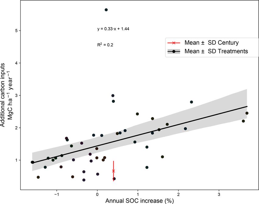
E. Bruni et al.: Additional carbon inputs to reach a 4 per 1000 objective in Europe                                                                                                                                   3985

Figure 1. Location of the 60 field trials distributed among the 14 cropland experiments around Europe.

Table 2. Information about experimental sites, including mean annual values of temperature (◦ C) and soil humidity to approximately 20 cm
depth (kgH2 O m−2                                                                                                             −3
                soil ) simulated with the ORCHIDEE model at each experimental site, measured pH, bulk density (g cm ), clay (%) and
initial SOC stocks in the control plots (Mg C ha−1 ) at the experimental sites. Reference papers for each site are indicated.

 Sites                       Reference paper                        Coordinates                   Years                     Mean annual           Mean annual            pH         Bulk         Clay       Initial SOC
                                                                                                                            temperature           soil humidity                   density                   stocks
                                                                                                                                          ◦C       kgH2 O m−2
                                                                                                                                                           soil                    g cm−3            %       Mg C ha−1
 Champ Noël 3a               Clivot et al. (2019)                   48.09◦ N, 1.78◦ W             1990–2008                             12.1                  21.6       6.3           1.35       15.1             40.57
 Colmar                      Levavasseur et al. (2020)              48.11◦ N, 7.38◦ E             2000–2013                              9.6                  24.6      8.33            1.3       23.1             54.33
 Crécom 3 PRO                Clivot et al. (2019)                   48.32◦ N, 3.16◦ W             1986–2008                             11.8                  22.9      6.15           1.36       14.6                62
 Feucherolles                Levavasseur et al. (2020)              48.88◦ N, 1.96◦ E             1998–2013                             11.9                  21.2      6.73           1.32       15.6             39.78
 Jeu-les-Bois                Clivot et al. (2019)                   46.68◦ N, 1.79◦ E             1998–2008                             12.2                  22.1      6.27           1.52         10             48.53
 La Jaillière 2 PRO          Levavasseur et al. (2020)              47.44◦ N, 0.98◦ W             1995–2009                             12.7                  20.5       6.8           1.37       20.8             32.42
 Le Rheu 1a                  Clivot et al. (2019)                   48.09◦ N, 1.78◦ W             1994–2009                             12.2                  21.8      5.85           1.27       16.4             36.23
 Le Rheu 2a                  Clivot et al. (2019)                   48.09◦ N, 1.78◦ W             1994–2009                             12.2                  21.8      6.05           1.28       13.9             36.53
 Arazurib                    –                                      42.81◦ N, 1.72◦ W             1993–2018                             12.7                  20.4       8.6           1.67       27.9             55.39
 Ultuna                      Kätterer et al. (2011)                 59.82◦ N, 17.65◦ E            1956–2008                              5.7                  22.6      6.23            1.4       36.5             41.72
 Broadbalk                   Powlson et al. (2012)                  51.81◦ N, 0.37◦ W             1968–2015                             10.2                  21.5       7.8           1.25         25             24.84
 Foggia                      Farina et al. (2017)                   41.49◦ N, 15.48◦ E            1992–2008                             15.5                  22.4       8.1           1.32         41             63.22
 Trévarez                    Clivot et al. (2019)                   48.15◦ N, 3.76◦ W             1986–2008                             11.8                  23.4      6.01           1.48       19.2            115.33
 Avrilléa                    Clivot et al. (2019)                   47.50◦ N, 0.60◦ W             1983–1991                             12.0                  20.2      6.59            1.4       17.6             54.46
a These experiments were part of the initial French database (AIAL) described in Clivot et al. (2019), but they were not selected for the final modeling work of this latter study. For more information, see also Bouthier
et al. (2014). b For Arazuri, data were directly provided by the Spanish Mancomunidad de la Comarca de Pamplona.

5.85 in Le Rheu 1 to a maximum of 8.33 in Colmar. The aver-                                                        It should be noted that the application of EOMs might in-
age bulk density (BD) in the control plots was 1.38 g cm−3 .                                                       duce differences in BD with time, which in turn affects the
SOC stocks (Mg C ha−1 ) were calculated at each site using                                                         calculations of SOC stocks. No adjustment was made in this
the following equation:                                                                                            sense, since data on the evolution of BD were available only
                                                                                                                   for a few sites. This might explain differences between the
SOC (Mg C ha−1 ) = SOC (%) · BD (g cm−3 )
                                                                                                                   SOC stocks calculated for Broadbalk in this paper and those
                                    · sampling depth (cm),                                           (1)           found by Powlson et al. (2012) at the same site, by adjusting
where SOC (%) is the concentration of organic C in the soil,                                                       soil weights to observed decreases in top soil BD due to accu-
and BD is the average bulk density of the experimental plot.                                                       mulating farmyard manure (FYM). Initial SOC stock values

https://doi.org/10.5194/bg-18-3981-2021                                                                                                                    Biogeosciences, 18, 3981–4004, 2021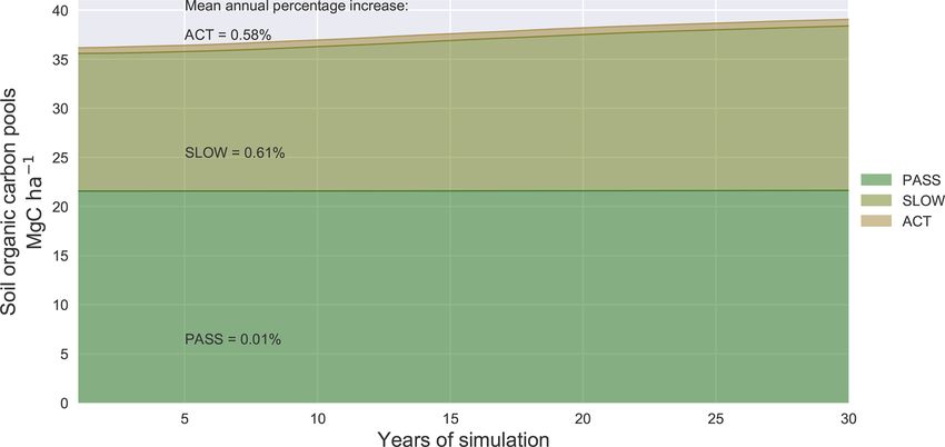
3986 E. Bruni et al.: Additional carbon inputs to reach a 4 per 1000 objective in Europe
in the aboveground (AG) plant material (Redin et al., 2014)
and 0.4 g C (g DM)−1 in the belowground (BG) part material
(Bolinder et al., 2007). We used the asymptotic equation of
Gale and Grigal (1987) to determine the cumulative BG input
fraction from the soil surface to a considered depth:
BGF depth = 1 − β depth , (2)
where β is a crop-specific parameter determined using the
root distributions for temperate agricultural crops, reported
in Fan et al. (2016) and Clivot et al. (2019). The depth was
set to 30 cm, since it was the depth at which soil samples
were taken at the majority of the sites. For more details on
the C input allocation method and the allometric functions
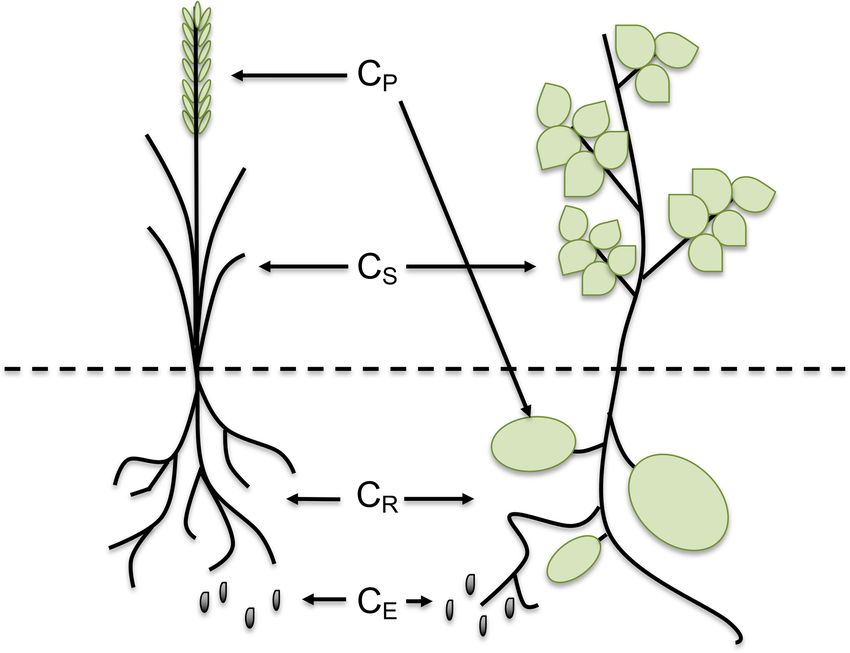
Figure 2. Adapted from Bolinder et al. (2007). Representation of involved, see Bolinder et al. (2007) and Clivot et al. (2019).
the distribution of carbon in the different parts of the plant: CP rep-
resents the carbon in the harvested product (grain, forage, tuber), CS 2.2 Century model
is the carbon in the aboveground residue (straw, stover, chaff), CR
is the carbon present in roots and CE represents all the extra-root 2.2.1 Model description
carbon (including all root-derived materials not usually recovered
in the root fraction). For this study, we selected the Century model, which has
proven to be well suited to accurately simulate the soil C dy-
namics in a range of pedoclimatic areas and cropping sys-
in the control plot and mean climate variables for each site tems (Bortolon et al., 2011; Cong et al., 2014; Parton et al.,
are reported in Table 2. 1993), and because we had the full command of the model
for fine tuning of parameters. Soil C dynamics in a soil or-
2.1.3 Carbon inputs ganic matter (SOM) model with first-order kinetics can be
mathematically described by the following first-order differ-
The allocation of C in the aboveground and belowground
ential matrix equation:
parts of the plant was estimated with the approach first de-
scribed by Bolinder et al. (2007) for Canadian experiments dSOC(t)
and then adapted by Clivot et al. (2019) to the same French = I + A · ξ TWLCl (t) · K · SOC(t), (3)
dt
sites we use in this study. This methodology allows the split-
ting of C inputs from crop residue after harvest into above- where I is the vector of the external C inputs to the soil
ground and belowground C inputs, using measured dry mat- system, with four nonzero elements (Fig. 3). The second
ter yields and estimations of the shoot-to-root ratio (S : R) term A·ξ TWLCl (t)·K·SOC(t) of the equation represents or-
and harvest indexes (HI) of the crops (see Fig. 2). The above- ganic matter decomposition rates (diagonal matrix K), losses
ground plant material is estimated as the harvested part of the through respiration (ξ TWLCl (t)), transfers of C among differ-
plant (CP ), which is exported from the soil, plus the straw ent SOC pools (A) and SOC evolution with time (SOC(t))
and stubble that are left in the soil after harvest (CS ). The (see Appendix A). We used the daily time-step version of
harvested part consists of the measurements of DM yields the SOM model Century (Parton et al., 1988) to simulate the
(YP ), while the straw and stubble are estimated using the amount of C inputs required to reach a 4 ‰ annual increase
HI coefficient of the different crops in the rotation (Bolinder in SOC stocks over 30 years. In the version used, only SOC is
et al., 2007). We assumed that the values used in Clivot et al. modeled, and plant growth is directly accounted for as vari-
(2019) for the HI compiled from French experimental sites ations in C inputs. The original version of Century simulates
were applicable to all the sites in our dataset, which mainly the fluxes of SOC depending on soil relative humidity, tem-
include temperate sites over Europe. When these values were perature and texture (as a percentage of clay). As shown in
not available for some crops, they have been directly derived Fig. 3, the model is discretized into seven compartments that
from Bolinder et al. (2007) or other sources in the litera- exchange C with each other: four pools of litter (aboveground
ture (S : R ratio for fallow from Mekonnen et al., 1997, and metabolic, belowground metabolic, aboveground structural
tomato from Lovelli et al., 2012). When straw was exported and belowground structural) and three pools of SOC (active,
from the field, we considered that only a fraction of CS was slow and passive). The litter C is partially released to the at-
left on the soil. This fraction was set to 0.4 for all sites and to mosphere as respired CO2 and partially converted to SOM
0.2 in Ultuna, where almost no stubble was left on the soil, in the active, slow and passive pools (see Table S1 in Sup-
since plots were harvested by hand and crops were cut at the plement for default Century parameters). The decomposition
soil surface. We considered a C content of 0.44 g C (g DM)−1 rate of C in the ith pool depends on climatic conditions and
Biogeosciences, 18, 3981–4004, 2021 https://doi.org/10.5194/bg-18-3981-2021E. Bruni et al.: Additional carbon inputs to reach a 4 per 1000 objective in Europe 3987
Figure 3. Representation of litter and soil organic carbon (SOC) pools in Century. The model takes as input litter carbon from plants
(aboveground metabolic (I1 ), belowground metabolic (I2 ), aboveground structural (I3 ) and belowground structural (I4 )). A certain fraction
of carbon can be transferred from one pool to another, and each time a transfer occurs, part of this carbon is respired and leaves the system
to the atmosphere as CO2 . The SOC active pool receives carbon from each litter pool, while only the structural material is transferred to the
SOC slow pool. Litter material never goes directly to the SOC passive pool while the three SOC pools exchange C within each other.
litter and soil characteristics and is calculated using environ- from steady state (Sanderman et al., 2017). Then, initializa-
mental response functions, as follows: tion can be done either by running the model iteratively for
thousands of years to approximate the steady-state solution
ξTWLCl (t)i · Ki = ki · fT (t) · fW (t) · fL i · fClay i , (4) (numerical spin-up) or semi-analytically by solving the set
of differential equations that describes the C transfers within
where i = 1, . . ., 7 is one of the AG and BG metabolic and
model compartments (Xia et al., 2012). We solved the matrix
structural litter pools and the active, slow and passive SOC
equation by inverse calculations for determining pool sizes at
pools; Ki is the (K)ii element of the diagonal matrix K in
steady state, as in Xia et al. (2012) and Huang et al. (2018).
Eq. (3); ki is the specific mineralization rate of pool i; fT (t)
These authors demonstrated that the matrix inversion ap-
is a function of daily soil temperature; fW (t) is a function
proach exactly reproduces the steady state and SOC dynam-
used as a proxy to describe the effects of soil moisture; fL i
ics of the model. By speeding up the performance of the sim-
is a reduction rate parameter acting on the AG and BG struc-
ulations, this technique allowed us to perform the optimiza-
tural pools only, depending on the lignin concentration in the
tion of model parameters, the sensitivity analysis of SOC to
litter; and fClay i is a reduction rate function of clay on SOC
climatic variables and the quantification of model output un-
mineralization in the active pool. The temperature function
certainties through Monte Carlo (MC) iterative procedures.
fT (t) describes the exponential dependence of soil decom-
We solved the matrix equation by using its semi-analytical
position on surface temperature, through the Q10 relationship
solution and the following algorithm: (1) calculating annual
that was first presented by M. J. H. van ’t Hoff (1884):
averages of matrix items obtained by Century simulations,
(T (t)−Tref ) driven by 30 years of climatic forcing, and (2) setting Eq. (3)
10
fT (t) = Q10 , (5) to zero to solve the state vector SOC. For each agricultural
site, the 30 years of climate forcing were set as the 30 years
where Q10 is the temperature coefficient, usually set to 2, and
preceding the beginning of the experiment, and the litter in-
Tref is the reference temperature of 30 ◦ C. The Q10 factor is a
put estimated from observed vegetation was set to be the av-
measure of the soil respiration change rate as a consequence
erage litter input in the control plot over the experiment du-
of increasing temperature by 10◦ . The other environmental
ration.
response functions are described in Appendix A.
2.2.2 Model initialization 2.2.3 Model calibration: optimization of the
metabolic : structural fractions of the litter inputs
The initialization of the model consists of specifying the
sizes of the SOC pools at the beginning of the experiment. In the Century model, AG and BG carbon inputs are further
Here, we assumed initial pools are in equilibrium with C in- separated into metabolic and structural fractions, according
puts before the experiments begin, in absence of knowledge to the lignin-to-nitrogen (L : N) ratio. Because the L : N ra-
about past land use and climate making initial pools different tio was not available for all the crops in the database, we
https://doi.org/10.5194/bg-18-3981-2021 Biogeosciences, 18, 3981–4004, 20213988 E. Bruni et al.: Additional carbon inputs to reach a 4 per 1000 objective in Europe
Table 3. Optimized values of the aboveground metabolic (AM), aboveground structural (AS), belowground metabolic (BM) and belowground
structural (BS) fractions of the litter inputs and the Q10 and reference temperature (◦ C) parameters.
Site AM AS BM BS Q10 Reference temperature
◦C
CHNO3 0.85 0.15 0.26 0.74 5.0 21.2
COL 0.85 0.15 0.57 0.43 2.0 30.0
CREC3 0.15 0.85 0.29 0.71 2.0 30.0
FEU 0.85 0.15 0.52 0.48 5.0 21.6
JEU 0.85 0.15 0.52 0.48 5.0 21.6
LAJA2 0.85 0.15 0.72 0.28 5.0 21.5
RHEU1 0.85 0.15 0.49 0.51 5.0 21.3
RHEU2 0.85 0.15 0.32 0.68 5.0 21.3
ARAZ 0.53 0.47 0.53 0.47 3.0 30.0
ULTU 0.85 0.15 0.85 0.15 2.2 30.0
BROAD 0.42 0.58 0.15 0.85 2.9 30.0
FOGGIA 0.15 0.85 0.15 0.85 5.0 27.1
TREV1 0.15 0.85 0.15 0.85 5.0 23.0
AVRI 0.85 0.15 0.76 0.24 2.0 30.0
fitted model simulations to observed SOC dynamics for the 2.2.4 Model calibration: optimization of temperature
control plot of each site, i.e. the reference plot without addi- dependency parameters
tional C inputs, in order to get the metabolic : structural (M :
S) fraction of the AG and BG carbon inputs. We used the We optimized the Q10 and daily soil reference temperature
sequential least-squares quadratic programming function in parameters, which affect SOC decomposition. The Q10 fac-
Python (SciPy v1.5.1, scipy.optimize package with method, tor is fixed to 2 in Century. However, many authors have
SLSQP), a nonlinear constrained, gradient-based optimiza- shown that Q10 measurements vary with pedoclimatic con-
tion algorithm (Fu et al., 2019). We successfully performed ditions and vegetation activity (Craine et al., 2010; Lefèvre
the optimization at 13 sites, where at least three measures of et al., 2014; Meyer et al., 2018; Wang et al., 2010). For this
SOC stocks were available. For Jeu-les-Bois, which includes reason, and to correctly reproduce interregional variations
two SOC measurements only, we decided to use the same among the sites in the dataset, we optimized both the Q10 and
optimized values as for Feucherolles, which has similar pe- reference temperature parameters to better fit the SOC dy-
doclimatic conditions and crop rotations. The optimization namics ( Mg C ha−1 ) of each agricultural site at the control
consisted in minimizing the following function: plot. We decided to bind the Q10 between 1 and 5, follow-
ing the variation in Q10 found by Wang et al. (2010) over
2
Xn SOCmodel − SOCobs 384 samples collected in the Northern Hemisphere. The ref-
i i
Jfit = i=1 SOCobs
, (6) erence temperature ranged between 10 and 30 ◦ C. We used
σ 2i the SLSQP optimization algorithm and the cost function of
Eq. (6) to perform the optimization, which was successful at
where i = 1, . . ., n is the year of the experiment, SOCmodel
i 13 sites, and we assigned the values obtained from the op-
(Mg C ha−1 ) is the SOC simulated with Century for year i,
timization of Feucherolles to Jeu-les-Bois, where SOC mea-
SOCobs
i (Mg C ha−1 ) is the observed SOC for year i in the
SOC
surements were too sparse to perform a two-dimensional op-
control plot and σ 2 i obs is the variance of the SOCobs i esti- timization. Optimized values of Q10 and reference tempera-
mated from the different replicates. When replicates were not ture are reported in Table 3.
SOCobs
available, we recalculated σ 2 as the variance amongst Model performance in the control plot was evaluated us-
obs ing two residual-based metrics. The first one is the mean
SOC samples of the whole experiment. The optimized
M : S values are reported in Table 3 and represent the aver- squared deviation (MSD), decomposed into its three compo-
age quality of litter C in the rotating crops along the duration nents to help locate the source of error of model simulations:
of the experiments that match control SOC data at each site. the squared bias (SB), the non-unity slope (NU) and the lack
of correlation (LC). The second metric used is the normalized
root-mean-squared deviation (NRMSD) (see Appendix B).
Biogeosciences, 18, 3981–4004, 2021 https://doi.org/10.5194/bg-18-3981-2021E. Bruni et al.: Additional carbon inputs to reach a 4 per 1000 objective in Europe 3989
2.3 4p1000 analysis N times, each time using one of the generated vectors I as a
prior for the optimization. To correctly assess the uncertainty
2.3.1 Optimization of C inputs to reach the 4p1000 over the required C inputs, we set N to 50 (Anderson, 1976).
target The SE of model outputs was calculated with Eq. (8), where
the variance was set as the variance of the modeled carbon
After the spin-up to steady state, the model was set to cal- outputs and the experiment size (s) to 50.
culate the SOC stock dynamics of the control plot and the
C inputs for virtual treatments, assuming an average increase 2.3.3 Analysis of sensitivity to temperature
in SOC stocks by 4 ‰ yr−1 over 30 years. A total of 30 years
is considered a period of time over which the variation in We tested the sensitivity of model outputs to tempera-
SOC can be detected correctly. During this period length, we ture, running two simulations with increased temperatures.
supposed the soil was fed with constant amounts of C in- We considered two representative concentration pathways
puts from plant material. For the control, we derived C in- (RCPs) of global average surface temperature change pro-
puts from measurements of DM yields and calculated the an- jections (IPCC, 2015). The first scenario (RCP2.6) is the one
nual mean over the whole experiment length. For the virtual that contemplates stringent mitigation policies and predicts
treatments, we used an optimization algorithm to calculate that average global land temperature will increase by 1 ◦ C
the required amount of C inputs to reach a linear increase in during the period 2081–2100, compared to the mean temper-
SOC storage by 4 ‰ yr−1 above the SOC stock at the start of ature of 1986–2005. The second scenario (RCP8.5) estimates
the simulation. Mathematically, we minimized the following an average temperature increase of +4.8 ◦ C, compared to the
function: same period of time. We ran two simulations of increasing
temperature scenarios with Century. We considered the same
J4p1000 = |SOC0 · (1 + 0.004 · 30) − SOCmodel
30 (I )|, (7)
initial conditions as the standard simulations, hence running
where I is the 1 × 4 vector of C inputs to minimize over, the spin-up with the average soil temperature and relative hu-
SOC0 is the initial SOC stock and SOCmodel 30 (I ) is the SOC midity of the 30 years preceding the experiments. Then, we
stock after 30 years of simulation. During the optimization, increased daily temperature by 1 ◦ C (AS1) and 5 ◦ C (AS5)
the M : S fractions were allowed to vary to estimate the qual- for the entire simulation length, to assess the sensitivity of
ity of the optimal C inputs. Instead, we kept the AG : BG ratio modeled C inputs to increasing temperatures. Nevertheless,
of the C inputs fixed to its initial value, to bind the model in it must be noted that our simulations are running over a 30-
order to represent agronomically plausible C inputs. In fact, year period, not the entire 21st century. Thus, the tempera-
if not bound, the model tends to increase the BG C fraction ture sensitivity analysis should not be considered a test of
to unrealistic values (assuming the same crop rotations per- climatic scenarios but a classical sensitivity analysis where
sisted on site). On the other hand, keeping the AG : BG ratio the boundaries were defined following RCP2.6 and RCP8.5
fixed implies that the simulated additional C inputs will be predictions of increased temperatures.
spread equally on the surface and belowground. As for the
previous optimizations, we used the Python function SLSQP
to solve the minimization problem. The outcome of the opti- 3 Results
mization is a 4 × 1 vector (I opt ) representing the amount of
3.1 Fit of calibrated model to control SOC values
C in the four litter input pools that matches the 4p1000 rate
target. Modeled and measured SOC stocks in the control plot were
compared to evaluate the capability of the calibrated version
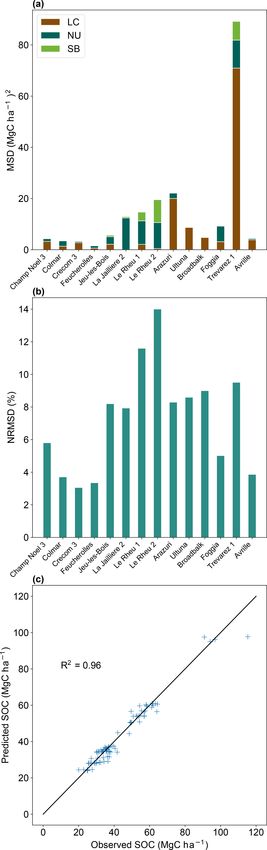
2.3.2 Uncertainty quantification
of Century to reproduce the dynamics of SOC stocks at the
Uncertainties of model outcomes were quantified using a selected sites (Fig. 4c). As shown in Fig. 4b, the NRMSD
Monte Carlo approach. We initially calculated the standard of the control plot SOC stocks is lower than 15 % for all the
error (SE) of the mean C inputs derived from yield measure- treatments, indicating that overall model simulations fitted
ments for each experimental site: the observed SOC stocks well (observed SOC stock variance
s was 16.3 % on average in the control plots). The correlation
σI2 coefficient between modeled and observed SOC stocks in the
SE = , (8) control plots was 0.96 (Fig. 4c). Figure 4a provides the values
s
of the three components of the MSD indicator for each site. It
where σI2 is the variance of the estimated C input from can be noticed that the LC and NU components are the high-
yield measurements and s is the length of the experiment. If est contributors to MSD. This means that the major sources
not available, we calculated σI2 as the average relative vari- of error are the representation of the data shape and mag-
ance of C inputs among the control plots. We therefore ran- nitude of fluctuation among the measurements. The highest
domly generated N vectors of C inputs (I ) around the calcu- NRMSD can be found at Le Rheu 1 and Le Rheu 2 (around
lated standard error and performed the 4p1000 optimization 12 % and 14 %, respectively). At these sites the model seems
https://doi.org/10.5194/bg-18-3981-2021 Biogeosciences, 18, 3981–4004, 20213990 E. Bruni et al.: Additional carbon inputs to reach a 4 per 1000 objective in Europe
Figure 5. Correlation between additional carbon inputs (Mg C ha−1
per year) and annual SOC stock increase (%) in the carbon input
treatments and mean ± standard deviation of the additional carbon
inputs to reach the 0.4 % target in Century.
to better capture the shape of the data (low LC compared to
the other sites), but it misses the representation of mean SOC
stock (high SB) and data scattering (high NU) of the experi-
mental profiles. We tested the capability of Century to repro-
duce SOC stock increase in the additional C input treatments
(Fig. 5). Figure 5 shows the correlation between additional
C inputs and SOC stock increase in the C input treatments
(R 2 = 0.23). In the same graph, we can appreciate additional
C inputs simulated by Century to reach the 4p1000 target be-
ing 0.66 ± 0.23 Mg C ha−1 yr−1 (mean ± standard deviation
from the mean). This shows that Century generally overes-
timates the effect of additional C inputs on SOC stock in-
crease. However, the effect of additional C inputs on ob-
served SOC stock increase varies largely across different
treatments.
3.2 Estimates of additional carbon inputs and SOC
changes
3.2.1 Virtual C inputs to reach the 4p1000
Figure 6 represents the average percentage change of C in-
puts required to reach the 4 ‰ annual increase in SOC
stocks, among all the sites. The increase in C inputs is
given for each litter pool. On average, a 43.15 ± 5.05 %
(mean ± SE across sites) increase in total annual C inputs
Figure 4. (a) Decomposed mean squared deviation (Mg C ha−1 )2 compared to the current situation in the control plot is re-
in control plots for all sites. LC: lack of correlation; NU: non-unity quired to meet the 4p1000 target. In terms of absolute val-
slope; SB: squared bias. (b) Normalized root squared deviation (%)
ues, this represents an additional 0.66 ± 0.23 Mg C ha−1 in-
in control plots for all sites. (c) Fit of predicted vs. observed SOC
stocks (Mg C ha−1 ) to control plots for all sites (R 2 = 0.96).
puts per year, i.e., 2.35 ± 0.21 Mg C ha−1 total inputs per year
(equivalent to approximately 4.05 ± 0.36 MgDM ha−1 yr−1 ).
What stands out in the graph is that, on average among
the studied sites, the AG structural litter pool should be
Biogeosciences, 18, 3981–4004, 2021 https://doi.org/10.5194/bg-18-3981-2021E. Bruni et al.: Additional carbon inputs to reach a 4 per 1000 objective in Europe 3991
Figure 6. Site average percentage change of carbon inputs needed to reach the 4p1000 (TOT), separated into the four litter input pools. AM:
aboveground metabolic; BM: belowground metabolic; AS: aboveground structural; BS: belowground structural; TOT: total litter inputs. Error
bars indicate the standard error. N.B: total change of carbon inputs (TOT) was calculated as the percentage change between the total amount
of carbon inputs before and after the 4p1000 optimization, averaged across all sites.
more than doubled, while the other pools need only to in- site relationship can be written as
crease by about half of their initial value. In terms of abso-
lute values, the structural AG biomass (which was initially I 4p1000 = 0.013 · SOCobs
0 + 0.001, (9)
0.29 Mg C ha−1 yr−1 on average in the control treatments)
would need an additional 0.18 Mg C ha−1 yr−1 to reach the where I 4p1000 represents the simulated C inputs needed
4p1000, the metabolic AG (initially 0.70 Mg C ha−1 yr−1 to reach the 4p1000 target (Mg C ha−1 yr−1 ) and SOCobs
0
on average) needs an additional 0.14 Mg C ha−1 yr−1 and (Mg C ha−1 ) is the observed initial SOC stock.
structural and metabolic BG biomass (initially 0.65 and
3.2.2 Virtual vs. actual C inputs in the experimental
0.52 Mg C ha−1 yr−1 ) require an additional C input corre-
carbon treatments
sponding to 0.21 and 0.13 Mg C ha−1 yr−1 , respectively.
Analysis of the SOC pool evolution in the runs with opti- In Fig. 9 we compare the C inputs required to reach the
mized C inputs to match the 4p1000 increase rate indicates 4p1000 target to the actual inputs used across the 46 treat-
that the active and slow pools increased by 0.58 % yr−1 and ments of additional C. The additional C (Mg C ha−1 yr−1 )
0.61 % yr−1 , respectively, while the passive pool increased shown in the graph for all experimental treatments refers to
annually by 0.01 % (Fig. 7). In absolute values, the slow exogenous organic amendments, plus additional C due to in-
compartment contributed the most to the increase in SOC creased crop yields, relative to the control plot. The most
during the 30-year runs, as it increased by 2.7 Mg C ha−1 striking result emerging from the data is that modeled addi-
on average among the sites (against an increase of 0.1 and tional C inputs are systematically lower or similar to at least
0.06 Mg C ha−1 in the active and passive compartments, re- one treatment of additional C at all sites, except for Foggia.
spectively). This corresponds to a storage efficiency for the In the Foggia experiment, different crop rotations were com-
30 years of simulation of approximately 13.7 % in the slow pared, and no additional EOM was incorporated to the soil.
pool, compared to a storage efficiency of 0.5 % and 0.34 % Here, none of the rotations had sufficient additional C content
in the active and in the passive pools, respectively. (compared to the control wheat-only treatment) to meet the
We found a high linear correlation (R 2 = 0.80) between required C input level predicted by Century for a 4p1000 in-
observed initial SOC stocks and optimized C inputs (Fig. 8). crease rate. Overall, 86.91 % of the experimental treatments
It is logical and expected that for low initial SOC stocks in used higher amounts of C inputs compared to the modeled
steady state, a small increase in C inputs is sufficient to reach need of additional C inputs at the same site. For the other
the 4p1000 target. Conversely, when SOC is high at the be- treatments, the difference between simulated and observed
ginning of the experiment (e.g., Trévarez) much higher C in- additional C input was not significant. In the experimental
puts must be employed since our target increase rate is a rel- treatments 1.52 Mg C ha−1 yr−1 was applied on average, and
ative target. The regression line that emerges from the cross- SOC stocks were found to be increasing by 0.25 % yr−1 rel-
ative to initial stocks. Modeled additional C input to reach a
https://doi.org/10.5194/bg-18-3981-2021 Biogeosciences, 18, 3981–4004, 20213992 E. Bruni et al.: Additional carbon inputs to reach a 4 per 1000 objective in Europe
Figure 7. Sites average soil organic carbon pools (ACT: active; SLOW: slow; PASS: passive) evolution (Mg C ha−1 ) over the 30 years of
simulation to reach the 4p1000 target. In the graph the mean percentage increase is given for each SOC pool.
control plots. This represents an additional C input increase
of 11 % and 77 %, respectively, compared to the business-as-
usual scenario with current temperature setup (CURR). What
can be clearly seen in the graph is the increased amount of
C inputs required in Trévarez, where C inputs should more
than quadruple to reach the 4p1000 objective.
4 Discussion
4.1 Reliability of the Century model
The Century model has been widely used to simulate SOC
stock dynamics in arable cropping systems (Bortolon et al.,
2011; Cong et al., 2014; Kelly et al., 1997; Xu et al., 2011).
Optimizing the metabolic : structural ratio in the reference
Figure 8. Correlation between initial observed SOC stocks plots allowed us to initialize the C input compartments, since
(Mg C ha−1 ) and modeled carbon inputs needed to reach the 4p1000 no measurement of the L : N ratio was available. This al-
target (Mg C ha−1 yr−1 ). The correlation coefficient (R 2 ) is 0.80 lowed us to (1) take into account the average C quality of the
and the regression line is y = 0.013 · x + 0.001. litter pools in the different crop rotations and (2) correctly es-
timate the initial values of SOC stocks at the majority of the
sites. On the other hand, this could have influenced the pre-
0.4 % increase was 0.66 Mg C ha−1 yr−1 , on average among dicted redistribution of C in the additional C inputs required
the sites. to reach the 4p1000 (Fig. 6). We suggest that taking into ac-
count the historical site-specific land use could help initialize
3.3 Carbon input requirements with temperature SOC stocks without requiring any assumption regarding the
increase M : S ratio (e.g., with historically based equilibrium scenar-
ios as in Lugato et al., 2014). To further improve SOC stock
The temperature sensitivity analysis of the Century model simulations, we optimized the Q10 and reference tempera-
for the 4p1000 target framework is plotted in Fig. 10. The re- ture parameters on the control plots to account for the dif-
quired amount of C inputs to reach the 4p1000 target is likely ferent pedoclimatic conditions of the experimental sites and
to increase with increasing temperature scenarios. In partic- enhance model predictions of SOC stock dynamics (Craine
ular, C inputs will have to increase on average by 54 % in et al., 2010; Lefèvre et al., 2014; Meyer et al., 2018; Wang
the AS1 scenario of +1 ◦ C and 120 % in the AS5 scenario of et al., 2010). Although the dispersion of SOC stocks over
+5 ◦ C temperature change, relative to current C inputs in the time is not perfectly captured in the majority of the control
Biogeosciences, 18, 3981–4004, 2021 https://doi.org/10.5194/bg-18-3981-2021E. Bruni et al.: Additional carbon inputs to reach a 4 per 1000 objective in Europe 3993 Figure 9. Additional modeled carbon inputs (Mg C ha−1 yr−1 ) to reach the 4p1000 (grey bars) compared to additional carbon input treatments (colored bars) at each experimental site. Additional carbon inputs for field trials are calculated as the sum of organic fertilizers and the delta carbon inputs from crop yields (compared to the control plot). Additional carbon treatments are separated into different categories: BIO waste: biowaste compost, green manure, green manure and sewage sludge, and household waste; Cow manure: cow manure and farmyard manure (in Broadbalk and Ultuna), pig manure, poultry manure, sewage sludge; Rotations: different crop rotations, other organic amendments (OA): straw, sawdust, and peat (in Ultuna) and castor meal (in Broadbalk). The error bars shown are the standard errors computed with the Monte Carlo method. plots (see the high LC component of the MSD in Fig. 4), the found to be increasing on average in the additional C treat- simulations of SOC dynamics were improved by the opti- ments (0.25 % yr−1 with 1.52 Mg C ha−1 yearly additional mization of temperature-related parameters, and the NRMSD C inputs), this increase rate is lower than the 0.4 % increase was found to be lower than 15 % at all sites. Figure C2 shows in SOC stocks predicted by Century with lower amounts of that the optimization of temperature-sensitive parameters did virtual C inputs (0.66 Mg C ha−1 yr−1 ). This is pointed out in not significantly affect the required C input estimation for the Fig. 5, where we can see that predicted additional C inputs to current temperature scenario. This means that, although pa- reach the 4 ‰ are lower than the correlation line between ad- rameter optimization improved the simulation of SOC stocks ditional C inputs and SOC stock increase in field treatments. in the control plots, the final results are not affected by it. The The overestimation of the C input effect on SOC stocks in capability of Century to simulate SOC stocks in the simula- Century might be related to the assumption that SOC stocks tions of additional C treatments might be a major shortcom- are in equilibrium with C inputs at the onset of the experi- ing of modeling results. In fact, although SOC stocks were ment and to the high sensitivity of the model to C inputs. https://doi.org/10.5194/bg-18-3981-2021 Biogeosciences, 18, 3981–4004, 2021
3994                                      E. Bruni et al.: Additional carbon inputs to reach a 4 per 1000 objective in Europe

Figure 10. Temperature sensitivity analysis of carbon input increase (%) to reach the 4p1000 objective. CURR: business-as-usual simulation;
AS1: RCP2.6 scenario of +1 ◦ C temperature increase; AS5: RCP8.5 scenario of +5 ◦ C temperature change.

4.2     Increasing annual SOC stocks by 4p1000                             In our study, not only the quantity of C but also the qual-
                                                                        ity will need to change according to Century predictions.
4.2.1    Modeled carbon inputs to reach the 4p1000                      In fact, the predicted AG structural litter change was 3-fold
                                                                        higher than all other pools on average, representing an ad-
Century simulations estimated that annual C inputs should               ditional 0.18 Mg C ha−1 each year. A way for the farmer to
increase by 43 ± 5 % (SE) on average to reach the 4p1000                increase the structural fraction of the C inputs is to compost
target at the selected experimental sites, under the condition          the organic amendments that will be spread on the soil sur-
that the additional C inputs are equally distributed among              face. Increasing EOM in large quantities may not be pos-
the surface and belowground, in order to maintain the same              sible everywhere. First of all, the amount of organic fertil-
AG : BG ratio as at the beginning of the experiment. Martin             izers is limited at the regional scale. If farmers source ad-
et al. (2021) found similar values of required additional C in-         ditional EOMs elsewhere, only those EOMs that otherwise
puts to reach a 4p1000 target in French croplands (i.e., 42 %,          would be mineralized (e.g., burned) and not applied to land
that is 0.88 Mg C ha−1 yr−1 ). This is higher than the values           account as sequestration. Second, farmers may be prevented
found by Chenu et al. (2019) using default RothC 26.3 pa-               from applying high amounts of EOM because of the risk
rameters, who estimated a relative increase in C inputs in              of nitrate and phosphate pollution (Li et al., 2017; Piovesan
temperate sandy soils by 24 % and in temperate clayey soils             et al., 2009). Moreover, producing additional animal manure
by 29 %. Riggers et al. (2021) found that in 2095 a minimum             implies larger GHG emissions through animal digestion and
increase in C inputs by 45 % will be required to maintain               manure decomposition. Consequently, even if more manure
SOC stocks of German croplands at the level of 2014. How-               is returned to the soil, it will not necessarily result in climate
ever, they found that to increase SOC stocks by 4 ‰ yr−1 , a            change mitigation.
much higher effort will be required. That is, C inputs in 2095
will have to increase by 213 % relative to current levels.

Biogeosciences, 18, 3981–4004, 2021                                                         https://doi.org/10.5194/bg-18-3981-2021
You can also read