Generating Relative Pick Value in the NBA Draft and Predicting Success from College Basketball - Digital WPI
←
→
Page content transcription
If your browser does not render page correctly, please read the page content below
Worcester Polytechnic Institute
Digital WPI
Major Qualifying Projects (All Years) Major Qualifying Projects

March 2019

Generating Relative Pick Value in the NBA Draft
and Predicting Success from College Basketball
Jake Connor Scheide
Worcester Polytechnic Institute

Michael James Krebs
Worcester Polytechnic Institute

Follow this and additional works at: https://digitalcommons.wpi.edu/mqp-all

Repository Citation
Scheide, J. C., & Krebs, M. J. (2019). Generating Relative Pick Value in the NBA Draft and Predicting Success from College Basketball.
Retrieved from https://digitalcommons.wpi.edu/mqp-all/6770

This Unrestricted is brought to you for free and open access by the Major Qualifying Projects at Digital WPI. It has been accepted for inclusion in
Major Qualifying Projects (All Years) by an authorized administrator of Digital WPI. For more information, please contact digitalwpi@wpi.edu.
Generating Relative Pick Value in the NBA
 Draft and Predicting Success from College
 Basketball

 A Major Qualifying Project Report:
 submitted to the faculty of the

 WORCESTER POLYTECHNIC INSTITUTE

 in partial fulfillment of the requirements for the
 degree of Bachelor of Science

 by

 ____________________
 Michael Krebs

 ____________________
 Jake Scheide

Date:

Approved: _______________________
Professor Craig Wills, Major Advisor
MQP-CEW-1901

Abstract
This project analyzes existing basketball player performance metrics, and generates new metrics
providing context behind player statistics. Using these metrics, we create a chart quantifying the
value of each pick in the NBA Draft. Finally, we create machine learning models that predict the
likelihood of NBA success for NCAA student-athletes.

 i

Acknowledgements
We would like to thank Professor Wills for his encouragement of us to apply our technical
backgrounds to our shared love for basketball.
We would also like to thank the staff at basketball-reference.com, as their extensive database of
college and NBA players made this project possible.
We would finally like to thank Jimmy Johnson, Kevin Pelton, Dr. Aaron Barzilai, and the
numerous other analysts who’s work informed our own, providing guidance and comparisons.
We hope our work will make a meaningful contribution to the growing body of literature
involving sports data mining.

 ii
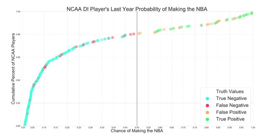
Table of Contents

Abstract ............................................................................................................................................ i
Acknowledgements ......................................................................................................................... ii
Table of Contents ........................................................................................................................... iii
Table of Figures .............................................................................................................................. v
Executive Summary ....................................................................................................................... vi
1. Introduction ................................................................................................................................. 1
2. Background ................................................................................................................................. 3
 2.1 Existing Metrics in the NBA ................................................................................................. 3
 2.2 Assessing Draft Value in Sports............................................................................................ 4
 2.2.1 NFL ................................................................................................................................. 4
 2.2.2 NBA ................................................................................................................................ 5
 2.2.3 Discussion ....................................................................................................................... 5
 2.3 Assessing Draft Value in the NBA ....................................................................................... 6
 2.4 Predicting NBA success based on college performance ....................................................... 8
 2.5 Summary ............................................................................................................................... 8
3. Design and Methodology .......................................................................................................... 10
 3.1 Determining Scope of the Project ....................................................................................... 10
 3.2 Collection and Manipulation of the Data ............................................................................ 10
 3.3 Analyze existing basketball player performance metrics .................................................... 10
 3.4 Feature engineer new player performance metrics addressing shortcomings with existing
 metrics ....................................................................................................................................... 11
 3.5 Find the highest value picks based on various measures of cost ........................................ 11
 3.6 Calculate the approximate value of every pick in the NBA Draft ...................................... 11
 3.7 Create a Jimmy Johnson-style NBA Draft value chart ....................................................... 11
 3.8 Summary ............................................................................................................................. 11
4. Results ....................................................................................................................................... 12
 4.1 Analyze existing basketball player performance metrics .................................................... 12
 4.2 Feature engineer new player performance metrics addressing shortcomings with existing
 metrics ....................................................................................................................................... 13
 4.2.1 Cumulative Individual Accolades ................................................................................ 13
 4.2.2 Basic Percentile ............................................................................................................ 15

 iii
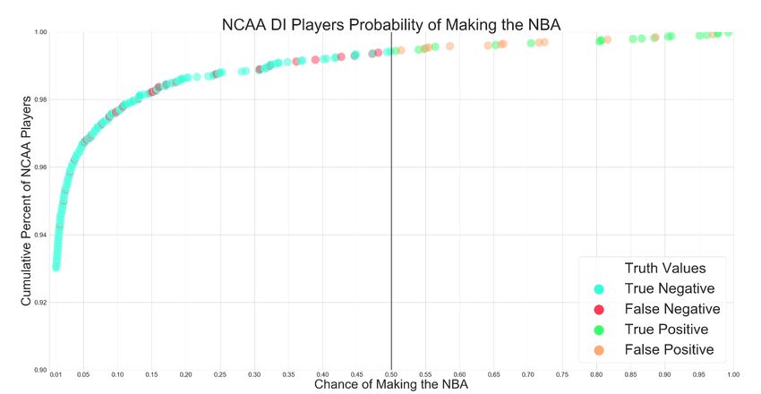
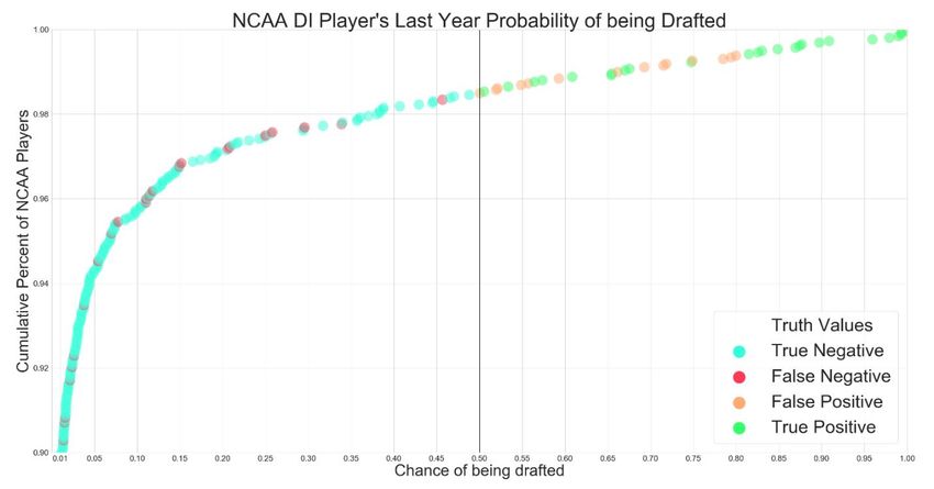
4.2.3 Advanced Percentile ..................................................................................................... 17
 4.3 Calculate the approximate value of every pick in the NBA Draft ...................................... 19
 4.4 Find the highest value picks based on various measure of cost .......................................... 22
 4.5 Create a Jimmy Johnson-style NBA Draft pick value chart ............................................... 23
5. Design and Methodology for NCAA ........................................................................................ 25
 5.1 Create a model which predicts various measures of NBA success based on NCAA DI
 statistics ..................................................................................................................................... 25
 5.2 Summary ............................................................................................................................. 27
6. Results for NCAA ..................................................................................................................... 28
 6.1 Using all seasons of NCAA DI players ............................................................................... 28
 6.2 Using only freshmen year seasons ...................................................................................... 32
 6.3 Using only a player’s last season ........................................................................................ 34
 6.4 Predicting on the 2019 NCAA DI Players .......................................................................... 36
7. Discussion ................................................................................................................................. 40
 7.1 Dataset ................................................................................................................................. 40
 7.1.1 Levels of Achievement ................................................................................................. 40
 7.1.2 Returning to College ..................................................................................................... 40
 7.2 Needle in a Haystack ........................................................................................................... 41
 7.3 Coefficients ......................................................................................................................... 41
8. Future Work .............................................................................................................................. 44
References ..................................................................................................................................... 45
Appendix A: Experiment Results ................................................................................................. 46
 Predicting whether an NCAA DI player will play an NBA game......................................... 46
 Predicting whether an NCAA DI player will be a lottery pick ............................................. 49
 Predicting whether an NCAA DI player will be a first round pick ....................................... 50
 Predicting whether an NCAA DI freshmen will be drafted .................................................. 52
 Predicting whether an NCAA DI freshmen will be a lottery pick ......................................... 53
 Predicting whether an NCAA DI freshmen will be a first round pick .................................. 54
 Predicting whether an NCAA DI player will play an NBA game ......................................... 55
 Predicting whether an NCAA DI player will be drafted ....................................................... 57
 Predicting whether an NCAA DI player will be a lottery pick ............................................. 59

 iv
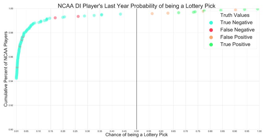
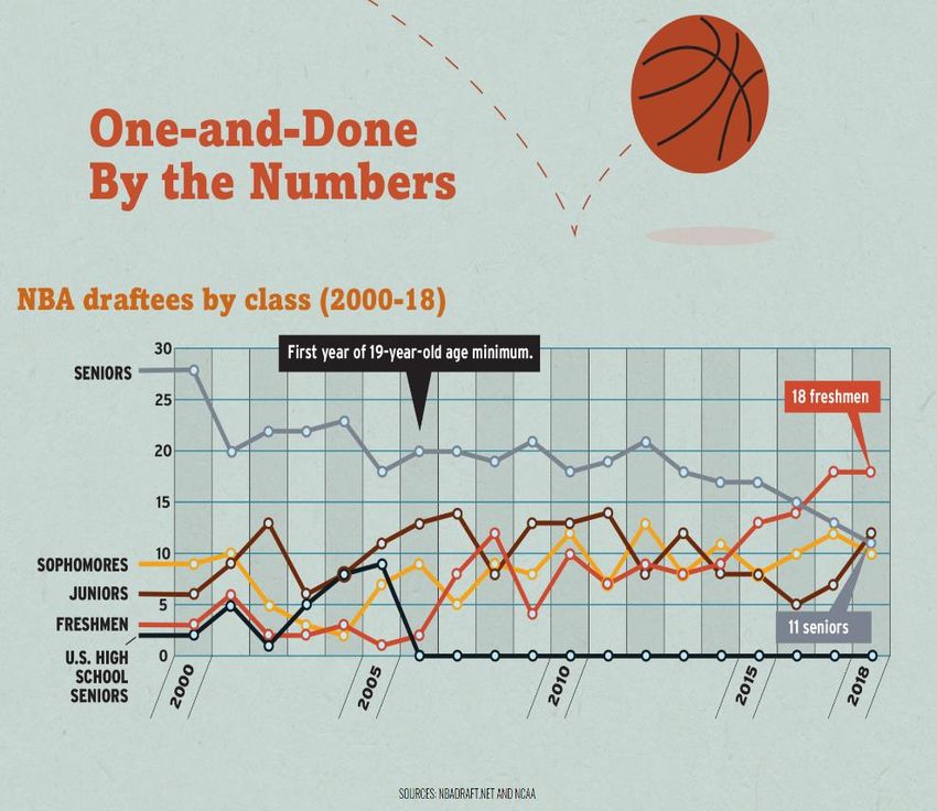
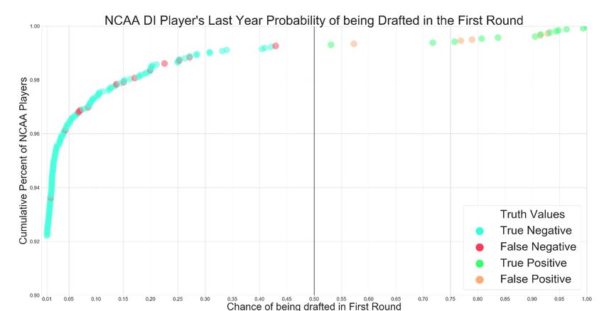
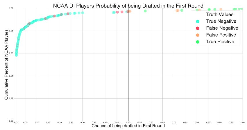
Table of Figures
Figure 1: Houston Rockets & New York Knicks Heatmaps .......................................................... 3
Figure 2: Jimmy Johnson Draft Table ............................................................................................ 4
Figure 3: Kevin Pelton Draft Table ................................................................................................ 5
Figure 4: Aaron Barzilai Career Relative Draft Value ................................................................... 7
Figure 5: Aaron Barzilai First 4 Years Relative Draft Value ......................................................... 7
Figure 6: Top 20 Players by existing metrics ............................................................................... 12
Figure 7: Existing metric Venn diagram ....................................................................................... 13
Figure 8: CIA Equation ................................................................................................................. 14
Figure 9: CIA Top 10 .................................................................................................................... 14
Figure 10: All metrics Venn diagram ........................................................................................... 15
Figure 11: Top 20 Basic Percentile ............................................................................................... 16
Figure 12: Top 20 Advanced Percentile ....................................................................................... 18
Figure 13: Career Cumulative Relative Value for NBA Draft ..................................................... 19
Figure 14: Clustered Career Relative NBA Draft Value .............................................................. 20
Figure 15: Trendline Clustered Cumulative Relative NBA Draft Value ...................................... 21
Figure 16: Value per dollar for NBA Rookies .............................................................................. 22
Figure 17: Mean Absolute Error of Draft Day Trades based on relative values .......................... 23
Figure 18: NBA Draft Relative Numeric Value ........................................................................... 23
Figure 19: NBA vs NFL Draft Value ........................................................................................... 24
Figure 20: Increasing numbers of freshmen in the NBA (Reynon, 2018) .................................... 26
Figure 21: Model experimentation results .................................................................................... 28
Figure 22: All NCAA season wasDrafted metrics ........................................................................ 29
Figure 23: All NCAA seasons wasDrafted breakdown ................................................................ 30
Figure 24: All NCAA seasons wasDrafted misses ....................................................................... 31
Figure 25: All NCAA seasons wasDrafted coefficients ............................................................... 32
Figure 26: NCAA Freshmen madeNBA metrics .......................................................................... 32
Figure 27: NCAA Freshmen madeNBA breakdown .................................................................... 33
Figure 28: NCAA Freshmen madeNBA misses ........................................................................... 33
Figure 29: NCAA Freshmen madeNBA coefficients ................................................................... 34
Figure 30: NCAA last season firstRound metrics......................................................................... 34
Figure 31: NCAA last season firstRound breakdown................................................................... 35
Figure 32: NCAA last season firstRound misses .......................................................................... 36
Figure 33: NCAA last season firstRound coefficients .................................................................. 36
Figure 34: 2019 NCAA player madeNBA predictions ................................................................. 37
Figure 35: 2019 NCAA players madeNBA probabilities ............................................................. 38

 v
Executive Summary
This project’s goals are threefold. First, we analyze existing basketball player performance
metrics, and use these insights to create new metrics that provide a better comparison for players
in the same season. Secondly, we generate a chart that quantifies the value of each pick in the
NBA Draft. Finally, we create machine learning models which predict if NCAA Division I
student-athletes will accomplish various levels of success in the NBA.

We used Player Efficiency Rating, Value Over Replacement Player, Win Shares and Fantasy
Points as our four established metrics. These metrics represent a spectrum of mechanisms that
front-offices, coaches, and fans use to evaluate and compare players. Often, these metrics tell
different stories about the talent of a player, and can be skewed by injury, players who take a
bench role later in their careers, or purely by nature of playing on a bad team. By examining the
factors that normalized these metrics, we constructed three additional player performance
metrics, with the goal of providing better insight into a comparison between two players in the
same season. These metrics were Cumulative Individual Accolades, Basic Percentile and
Advanced Percentile.

Using these metrics, we grouped players based on their selection in the NBA Draft, and created
visualizations showing the different ‘talent curves’. By clustering groups of picks together, we
created equations which smoothly estimated the value of each pick. We then collated draft pick
only trades made in the NBA since 2005 and settled on a best curve which accurately mapped
them. From this, we compared our talent curve for the NBA to both NBA and NFL models,
where these charts are actively used by teams for guidance in draft-pick trades.

Finally, we used machine learning to construct linear regression models that classify NCAA DI
players based on various success criteria for the NBA. The success criteria we were particularly
interested in were being drafted by an NBA team, drafted in the lottery / first round, and playing
in an NBA game. These models considered not only the basic and advanced statistics of the
players, but also the school they went to, height and weight. These models were extremely good
at identifying talented prospects, and many misclassified players were found to have extenuating
circumstances.

Overall, this project provides significant value to the front offices of NBA teams who are
attempting to maneuver around the uncertainty associated with the NBA Draft. Selecting the
right player is extremely important for a team’s long-term success, even with lower picks in the
draft. By understanding the true value of the team’s draft position, and utilizing models such as
our own, teams can make more informed draft decisions and extract the maximum value from
their picks.

 vi
1. Introduction
Basketball is exploding both domestically and abroad, with the most recent National Basketball
Association (NBA) season posting record attendance, TV and online viewership numbers
(Adgate, 2018). Players now come from 42 countries, with all 30 franchises having at least one
non-American player. The league is expanding their outreach into emerging markets such as
China, India and Africa, with 300 million people in China playing basketball (Saiidi, 2018). This
explosive growth has skyrocketed median team valuations, from $555 million in 2014 to over
$1.5bn in 2018 (Routley, 2019).

As the NBA has grown, so has the potential lucrativeness of constructing a championship-
winning roster. The Golden State Warriors, winners of three of the last four NBA
Championships, find themselves paying $90 million in ‘luxury tax’, an economic penalty on
teams which exceed the salary cap (Ramey, 2018). If they maintain their current roster, they will
pay $221 million in luxury taxes during the 2020-21 season, more than the actual payroll of $178
million. The Warriors show just how valuable winning in the NBA is, even when paying such
high taxes.

With this increased pressure to succeed (and therefore profit), teams must utilize every resource
at their disposal to ensure they are accurately evaluating players both at the professional and
collegiate level, the latter of which is the primary supplier of young NBA talent. The NBA Draft
is held at the end of every season, where each team is awarded two selections in the sixty-pick
event. Picks 15-60 are assigned in reverse order of record (where the best record team gets the
30 and 60 picks), and a lottery decides the recipients of the first fourteen picks, with
 th th

probabilities proportional to standings. Teams are free to trade their rights to a draft pick prior,
during, and after the draft lottery, as they try to maneuver up the draft board to obtain the best
young talents.

Some teams looking to contend for championships may trade all their draft picks away for
veteran contributors, as the Brooklyn Nets did in 2014. They traded three first round picks, as
well as the right to swap first round picks (in four consecutive years), to the Boston Celtics for
Kevin Garnett, Paul Pierce, and Jason Terry – three championship winning players who declined
rapidly following Brooklyn’s acquisition (Greenberg, 2017). The Celtics benefitted even more
from the players’ declines, as the struggling Brooklyn ended up receiving the third, first, and
eighth selections in the draft- only the rights to the picks belonged to the Celtics.

This project’s goals are threefold. First, we analyze existing basketball player performance
metrics, and use these insights to create new metrics that provide a better comparison for players
in the same season. Secondly, we generate a chart that quantifies the value of each pick in the
NBA Draft. Finally, we create machine learning models that predict if NCAA Division I student-
athletes will be drafted or play in the NBA.

This project is timely, relevant, and important to NBA teams which seek to improve their teams
through the draft, or trades. By analyzing player performance metrics, teams can contextualize
the numbers they often are presented with by their analytics departments when debating a

 1
prospective trade. Additionally, analytics professionals can supplement the metrics they currently
use with the ones we created, to generate more informed insights. When proposing or
deliberating on trades involving draft picks, teams can use our draft pick value chart to ensure
they are fairly compensated for the outgoing picks. Finally, front offices can verify their scouts’
opinions on a collegiate player using the machine learning models we created to ensure they are
selecting players who will be successful in the NBA.

In the remainder of this report, we first break down existing player performance metrics to better
understand the mechanisms used by NBA teams when performing trades and contract
negotiations. Using this understanding, we design three new player performance metrics that
provide a new approach to evaluating talent. By summating the metric values for a set of NBA
players, we then generate charts which approximate the relative value of each selection in the
NBA Draft. Using draft-pick only trades, we calculate the error of each relative value curve to
finally settle on one equation which explains the value of NBA draft picks. From our literature
review, we compare our value chart to other NBA charts, as well as numerous NFL value charts,
to compare the talent drop-off. Finally, using machine learning, we create models that predict if
NCAA DI basketball players will be drafted and/or play in the NBA. The models use statistical
data scraped from online sources, as well as the college the player attended, their height, and
their weight.

 2
2. Background
2.1 Existing Metrics in the NBA
Although many casual sports fans attribute the numbers revolution in sport to Moneyball,
statistics and data were driving decision making in sport from as early as the 1920’s, with
baseball initially pioneering the movement (Schwarz, 2004). Baseball is largely viewed as the
easiest game to quantify, as models can describe progress to scoring a run objectively with
players moving along the bases. Additionally, each pitch is an independent event, further
allowing itself to be analyzed using basic mathematics.

Basketball, on the other hand, is a free flowing, five on five game where missing an open layup
after a well-run play counts for the same on the score sheet as a highly contested long-range shot.
The complexity of basketball makes it a lot tougher to generate numbers which accurately reflect
the talent level of a player or team. Additionally, Dean Oliver posits, the lack of statistics readily
counted about defense makes basketball analytics largely skewed towards offensively-minded
players (Oliver, 2004). Oliver invented the ‘Four Factors’ most critical to team success in
basketball, namely shooting, rebounding, turnovers, and free throws. Each of the Four Factors
 are weighted differently and measured using
 advanced metrics. His book introducing these
 metrics, Basketball on Paper, is widely regarded as
 the bible of basketball analytics.

 Fast forward 15 years from the book’s publication
 date, and data has truly revolutionized basketball.
 Teams have discovered the value of the three-point
 shot, and offenses and teams are now constructed
 to find threes and layups (Shot Search, n.d.). It’s no
 coincidence that the teams investing the most in
 analytics, such as the Houston Rockets, are finding
 the most success. Figure 1 shows the large
 disparity in shot selection between the Rockets and
 the New York Knicks – a team languishing at the
 bottom of the NBA standings.

 An analysis of basketball metrics is not something
 novel, but past papers arbitrarily pick statistics to
 incorporate into their analysis (Mertz, et al., 2016).
 For example, including points, rebounds and assists
 in addition to Win Shares per 48 minutes double
 counts the basic points, rebounds and assists
 statistic. Any ranking of players will require
Figure 1: Houston Rockets & New York Knicks Heatmaps
 careful consideration of the basic statistics that go
 into the metrics used, as well as any possible
 normalizing factors used, such as minutes played, team wins, or pace of play.

 3
2.2 Assessing Draft Value in Sports
2.2.1 NFL
One of the project’s goals is identifying the value of draft picks in the NBA. In the NFL, there
exists a widely known draft value table constructed by former Dallas Cowboys head coach
Jimmy Johnson (Johnson, 2019). This draft table was designed to assess what a fair trade would
be when trading draft picks. The work done by Barney et. al showcased that draft pick trades did
in fact follow closely the values assigned in this draft value table. Indicating either the teams
used the draft table to decide if the trade was fair or the table accurately showcases relative
value for draft picks. In either case the most important aspect in determining if a draft table is
effective is if trades that are made reflect relative values given in the table. Figure 2 displays the
first 60 picks and their value from the Jimmy Johnson draft table.

Figure 2: Jimmy Johnson Draft Table

 4
2.2.2 NBA

However, unlike the NFL, the NBA does not have a publicly known draft value table. NBA draft
value tables do exist, one of which was created by ESPN staff writer Kevin Pelton. In Pelton’s
first draft value table, he confines the value of a pick to only the years played on the rookie
contract since unless that player is traded they will be providing value to the team they were
selected on (Pelton, Making smart, valuable trades to move up in the draft is harder than it looks,
2015). Pelton acknowledged that in doing so he decreases the value of a top pick because the
value they provide after the rookie contract is also likely more than lower picks. He remade his
draft value chart with the addition of looking at how players drafted between 2003-07 performed
in years 5-9 of their careers (Pelton, Trade down or keep No. 1 pick: Which is more valuable?,
2017). This time frame was considered because this would be the amount of time covered by a
maximum rookie extension. Figure 3 displays Kevin Pelton’s 2017 draft value table.

Figure 3: Kevin Pelton Draft Table

2.2.3 Discussion

 5
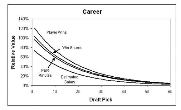
When comparing the two draft tables side by side, the values are similar. With the 7th pick
having the same relative value in each and the 15th pick having a percent difference of 12% in
relative value. The major difference between the two tables comes after these first 15 selections
as we transition into the latter half of the first round and into the second round for the NBA.
NBA players relative value drops below 10% of the first pick’s value at the 31st pick which is
the first pick of the second round. Contrast that with the first pick in the second round of the NFL
(33) which has a relative value of 19.33% of the first pick. These two picks have a percent
difference of 73% which is quite substantial. This large difference suggests that the drop off for
relative value in a pick decreases faster and steeper in basketball than they do in football.

A main reason for the large difference is there being less people on a team and playing at one
time in basketball than in football. In basketball there are more opportunities for a player to make
an impact when playing, since they are playing a large portion of the game. On the other hand, a
less skilled player has less opportunities to make an impact since only 5 players on the team are
on the court at one time. Considering only the regular season a basketball player can play for an
entire game for all 82 games (35 minutes for 75 games is more reasonable but the former is still
possible), whereas a football player is on the field for roughly half the game, if their offense is on
the field the same amount as the defense, if they play every snap for 16 games. Although a single
play or performance has a greater impact on the season outcome in football than in basketball; a
higher skilled basketball player will be able to provide more consistent value to their team over a
less skilled player to a greater effect than in football.

Furthermore, due to the shorter season and limited time on the field, lucky plays or breakout
performances are more likely to occur in football than in basketball. This narrows the gap
between how much value a great player vs. a good player can contribute over the course of a
season because a good player who gets lucky can provide more value to a team in a game than a
great player who is more consistent. Consider a highly skilled wide receiver who has 100 yards
receiving on 11 catches, but on all of those drives they failed to score any points. On the other
hand, a less skilled wide receiver who had one touchdown catch for 88 yards that was due to a
free safety tripping. In the context of the game, the great player provided more consistent value,
but the good player added 6 points to the team and would provide more value to their
team. Football is a lower scoring game than basketball so lucky plays in football like a “pick
six” have a huge effect on the outcome of the game and a lucky play in basketball can result in at
most 4 points which likely will not affect the game. This sample size issue can also be reflected
in baseball, where the 162-game season gives more context to the low likelihood of getting a hit.

2.3 Assessing Draft Value in the NBA

In 2007, Dr. Aaron Barzilai explored the often-overlooked topic of draft value in the National
Basketball Association (Barzilai, 2007). Dr. Barzilai assessed the value of each draft pick using 4
metrics (Player Efficiency Rating, Player Wins, Win Shares, and Estimated Salary) over 3
different time periods (career, first 4 years, and years with rookie team) for a total of 12 total
metrics. But Barzilai decided that estimated salary was only meaningful for the career time
period, so he considered only 10 metrics. Below are the regression lines for the metrics
excluding the years with rookie team due the large amount of variability caused by the differing
lengths players spend with their rookie team.

 6
Figure 4: Aaron Barzilai Career Relative Draft Value

 Figure 5: Aaron Barzilai First 4 Years Relative Draft Value

The work done by Dr. Barzilai shows that wins are correlated more to where a player was drafted
than PER. A player who was drafted highly, especially a lottery pick, will almost always see the
court for a long time. This can be attributed to the fact that higher picks go to lower performing
teams. These lower performing teams can take longer to develop these young players and the
talent on the team is lower, so the newly drafted player plays far more minutes than a later draft

 7
pick who is playing on a perennial playoff team. Although, for most cases a higher pick (earlier
selection) is a better player than a lower pick (later selection), there are instances where a later
pick will produce more value simply because they are given more chances and could be equally
as talented as a lower pick. These late round picks are referred to as steals in the draft and the
non-producing early picks are called busts. But in order to figure out if a player is a steal or a
bust, they need to have time on the court to showcase their talents. Due to a larger proportion of
higher picks getting playing time it makes sense that most people can think of examples of draft
busts but not many examples of draft steals. Looking forward, our project will attempt to better
quantify what value a player contributes to their team which may shine light on more draft steals.

2.4 Predicting NBA success based on college performance

In American professional sports leagues, drafts are conducted to introduce young talent fairly to
all teams. Generally, pick order is decided by inverse order of record, so that worse teams have
the first selections and the best chance at picking a superstar. While this system sounds airtight in
theory, equality has been increasingly vapid in the NBA. The teams with poor scouting
departments-whether it be from personnel or budget limitations-find themselves anchored to the
bottom of the standings and making early draft selections each year. Thus, the challenge is to
accurately identify successful players from leagues all over the world, using limited data.

Purely numerical statistics are not enough to evaluate a player, however. Players who struggle to
make NBA rosters have experienced incredible success in international leagues, with Jimmer
Fredette and Stephon Marbury two prime examples. The NCAA is the closest thing to a level
playing field NBA teams have to evaluate talent against, as amateur student-athletes play for
their college teams. Analysts have used numerical statistics and size in conjunction with
subjective scouting to try to predict professional success for collegiate players, to reasonable
success. Others try to directly find a relationship between college statistical production and NBA
production. What all past models have not done, however, is taking each unique school into
consideration when evaluating the likelihood of them making the NBA. Even within the same
conference, certain teams are far more likely to send players to professional leagues than others.

2.5 Summary
Overall, we understand that many schools of thought have produced many different numbers to
evaluate basketball players. Due to the game’s free-flowing nature, quantifying every effort a
player contributes to a team is extremely challenging. Only with recent advancements in player-
tracking data are teams beginning to find ways to measure defensive capability, and other factors
previously considered intangible.
For the specific application of the draft, relative value is a crucial component of the NFL
landscape, where the lengthy draft process leads to many draft pick-only trades. In the NBA,
there is a sizable gap in the analysis of draft value, and a lack of discussion regarding the most
important statistics to consider when evaluating a prospective talent. We designed our
experiments to address these gaps, providing draft value charts for the NBA with statistical rigor,
and discovering the most important factors for predicting NCAA DI athlete success in the NBA
using machine learning.

 8
9
3. Design and Methodology
3.1 Determining Scope of the Project
The NBA has had extensive changes to its rules, restrictions on eligibility and size as an
association since its creation. In order to best evaluate a modern-day player and produce metrics
for their value, it was imperative to consider the time period of the NBA we would include in our
dataset. We opted to use data from 1990-2018 in our project. The majority of NBA rules have
remained consistent during this timeframe, with one exception being the three-point line’s move
from 23 feet 9 inches uniformly to 22 feet in 1995 and subsequent extension at the top of the key
(corner remained at 22 feet) to 23 feet 9 inches. In the 1990’s, more rule changes altered the way
on-ball defense was played, removing the ability for the defender to ‘hand check’ the offensive
player. This change was implemented to aid offensive players, making the games higher scoring
and thus more entertaining. An important period captured in this dataset is the Jordan years of
the NBA. Although not a definitive time period, the NBA in the 90’s was focused on physical,
defensive play (as demonstrated by the Detroit Pistons’ “Bad Boys”) to a more offensive and
point producing league in the 2000’s, with the 3-point explosion revolutionizing the game in the
2010’s.

3.2 Collection and Manipulation of the Data
In order to collect the data for our project, we utilized web scraping techniques through the
Python package Beautifulsoup. We obtained our information from Basketball-Reference.com
which had all of the player data required for the analysis. To produce our dataset, we first
iterated through each season and then for each season pulled the player information from three
tables. Thee three tables were “per-game”, “total” and “advanced.” Each of these tables has
every player who played a game in that season within the table. Once all of these tables were
saved to local spreadsheets, we created functions that cumulatively combined the seasons of data
which outputted a single spreadsheet with per-game statistics, total statistics, and advanced
statistics for every player in every season they played in the NBA since 1990. To produce the
cumulative metric, we also needed to pull data on all-star selections and seasonal awards. We
again utilized basketball-reference as for each year they had tables of award summaries that
included all award-winning players. These awards were transformed into their own respective
column where a 1 indicated they achieved that award and a 0 meant they did not.

3.3 Analyze existing basketball player performance metrics
In professional sports, ‘value’ can be quantified in many ways. Some measures look purely at
statistical output, whereas others take factors such as contract cost, minutes played, and team
wins into account. To contextualize our entire project, which involves measuring the
performance of basketball players, we analyzed the common metrics used to evaluate players.
These four metrics were Player Efficiency Rating (PER), Win Shares (WS), Value over
Replacement Player (VORP) and Fantasy Points (FP).

 10
3.4 Feature engineer new player performance metrics addressing shortcomings with
existing metrics
After analyzing the existing player performance metrics, we identified potential areas for
improvement with different metrics that allowed for a more accurate comparison of players in
the same season. These metrics were called Basic Percentile (BP) and Advanced Percentile (AP).
Additionally, we created a metric which rewarded recognition rather than statistical output,
called Cumulative Individual Accolades (CIA).

3.5 Find the highest value picks based on various measures of cost
One of the most important applications of talent evaluation is the NBA Draft. Each of the thirty
teams are assigned two picks, generally in inverse order of team wins. A lottery is conducted for
the first fourteen picks, to disincentivize intentional losing of games (commonly referred to as
‘tanking’) to obtain a highly talented player with the first pick. The NBA rookie salary scale
provides an approximation of the talent level available at each pick, which we use with the
performance metrics to find the draft picks which provide the highest output per dollar.

3.6 Calculate the approximate value of every pick in the NBA Draft
Another possibility in the NBA Draft is pick trading. Both before and during the draft, teams can
swap picks for players or even high picks for multiple lower picks. As such, knowing the value
of each position in the draft is critical to teams trying to improve their talent. We use the
performance metrics to analyze the drop-off in talent at each pick in the draft.

3.7 Create a Jimmy Johnson-style NBA Draft value chart
Pick trading is far more common in the National Football League (NFL) where there are 224
picks between 32 teams. NFL Analyst Jimmy Johnson created a draft chart in the early 1990’s
which seeks to quantitatively evaluate the talent available at each pick. We apply this to the NBA
and create a value chart which accurately matches past draft pick trades in the NBA.

3.8 Summary
Overall, the key goals of this project section are to identify new avenues for basketball player
performance evaluation and using that knowledge to generate useful information regarding the
value of draft picks. We verify our approach through comparing the results to existing research
done in the NFL and NBA.

 11
4. Results
4.1 Analyze existing basketball player performance metrics
As discussed in the previous section, a crucial decision in evaluating player value is how
‘performance’ is quantified. Figure 6 lists the top 20 players ranked using the four existing
metrics, averaged out over the course of each player’s career.

Player WS PER VORP FP AVG Starting at the top, we can see that
LeBron James 1 2 1 1 1.3 there’s a reasonable consensus
Karl Malone 2 4 2 2 2.5 among the top three players.
David Robinson 4 1 4 5 3.5 Beyond that, the metrics begin
Tim Duncan 8 6 9 4 6.8 disagreeing quite significantly. For
Chris Paul 5 7 5 11 7.0 example, Michael Jordan earns
Kevin Durant 7 8 15 7 9.3 third place in Win Shares and
Shaquille O’Neal 14 3 18 3 9.5 VORP, but doesn’t feature in the
Michael Jordan 3 11 3 21 9.5 top 20 for Fantasy Points. Because
Charles Barkley 10 5 6 21 10.5 Win Shares distributes production
Russell Westbrook 21 16 8 6 12.8 by the number of wins the teams
Kevin Garnett 17 17 12 8 13.5 accrues, players on successful
John Stockton 6 13 19 16 13.5 teams (such as the 90’s Bulls,
Hakeem Olajuwon 21 10 17 10 14.5 arguably the greatest team ever)
James Harden 12 21 11 17 15.3 will feature strongly in the WS
Clyde Drexler 16 19 7 21 15.8 rankings. Similarly, Magic
Stephen Curry 15 21 10 19 16.3 Johnson’s extremely strong Lakers
Kobe Bryant 20 15 21 13 17.3 teams boosts his WS rank to 9,
Dirk Nowitzki 13 18 21 18 17.5 which is the only time he features in
Magic Johnson 9 21 21 21 18.0 these standings.
Dwight Howard 18 21 21 12 18.0
Yao Ming 21 9 21 21 18.0 Extrapolating from this chart, if
Allen Iverson 21 21 21 9 18.0 these metrics disagree so
Jason Kidd 21 21 16 15 18.3 significantly for the absolute best
Dwyane Wade 21 12 20 21 18.5 players, it’s likely that mediocre
Reggie Miller 11 21 21 21 18.5 players will also have large
Scottie Pippen 21 21 13 21 19.0 disparities in their statistical
Larry Bird 21 21 14 21 19.3 rankings by each metric.
Anthony Davis 21 14 21 21 19.3
Gary Payton 21 21 21 14 19.3
Jeff Hornacek 19 21 21 21 20.5
Amare Stoudemire 21 20 21 21 20.8
Patrick Ewing 21 21 21 20 20.8
 Figure 6: Top 20 Players by existing metrics

 12
To investigate just what these statistical
 disparities might be, we broke down each metric
 to its mathematical formula, to see their
 components. We were particularly interested in
 the components which normalized each metric,
 displayed in Figure 7.

 Fantasy Points is the most basic metric – it
 multiplies each basic ‘counting stat’ by a
 coefficient and outputs a number representing
 the volume of statistical output by a player. The
 coefficients seek to equalize the value of assists,
 rebounds, and points. FP does not consider the
 player’s efficiency, or pace of play. Obviously,
 20 points in a game ending 74-68 is more
 valuable than 25 points in a 135-123 game, but
 FP would rank the latter performance as
 stronger. By normalizing to pace, the metric
Figure 7: Existing metric Venn diagram would consider the amount of points the player
 scored per 100 possessions, allowing for a more
accurate comparison.

In that case, let’s now move to PER, a stat which is normalized to pace, as well as minutes
played. It multiplies counting stats by coefficients and analyzes the proportion of team field
goals the player’s assists contribute towards. Additionally, PER subtracts what its creator, John
Hollinger, calls “negative accomplishments” such as turnovers, personal fouls, and missed
defensive rebounds. PER’s largest flaw is its greatest strength- minutes normalization. Because
of limited sample size, the player with the all-time highest PER has only played a few minutes.
Adding minimum games or minutes played removes these outliers, but on the other end, players
who make significant contributions during their prime, only to decrease in efficiency in their
career’s twilight are prone to having a low career average PER.

As such, there is no true ‘best metric’ for evaluating talent. Undoubtedly, every player on this list
is a great player in their own right, but such significant difference in the ranking suggests there
might be a better way to evaluate talent.

4.2 Feature engineer new player performance metrics addressing shortcomings with
existing metrics

4.2.1 Cumulative Individual Accolades

When fans compare players, they often point to the number of individual awards a player accrues
over their career. With that in mind, we sought to quantify these awards by examining the
mathematical chance that a player accomplishes a certain milestone if all players were randomly
selected.

 13
The baseline accomplishment is being named in the 12 active players for each game, which we
assign one point to each player. From there, five players are named to the starting lineup (5/12),
which is equivalent to 2.4 points. We follow the same methodology for playing a minute on the
court, all the way to winning the MVP, which is a 1/450 chance (given 15 players on 30 teams’
rosters), thus awarding 450 points.
 12−1 5 −1 10−1
 = ∗ + ∗ + ∗
 12 12 24
 −1
 5 5 −1
 + ∗ + ∗
 450 450
 5 −1 1 −1 1 −1
 + ∗ + ∗ + ∗
 60 60 450
 −1 −1
 1 1 1 −1
 + ∗ + ∗ + 6
 450 450 210
Figure 8: CIA Equation

 Player 2018 CIA Figure 9 shows the top 10 players as ranked by CIA for
 Victor Oladipo 1242 2018. Victor Oladipo won Most Improved Player, made the
 James Harden 1152 All-NBA Defensive Team and the All-NBA Third Team.
 Rudy Gobert 976 James Harden won MVP and was named to the All-NBA
 Anthony Davis 835 First Team. Because the statistical likelihood of making the
 Lou Williams 832 Third Team is equivalent to making the First Team, it
 LeBron James 816 slightly muddies the data. Similarly, Most Improved Player
 Jrue Holiday 792 awards the same points as MVP. While this metric was an
 Karl-Anthony Towns 791 interesting twist on the typical in-game analysis of player
 Russell Westbrook 789
 performance, we found it to be inappropriate to further
 analyze players using this metric.
 Figure 9: CIA Top 10

 14
4.2.2 Basic Percentile
 There are five major ‘counting stats’ in basketball
 and are the basis for almost all stats as they tally a
 player’s basic contributions to their team. The five
 stats are points, assists, rebounds, blocks and steals.
 We felt that there was a need to develop a stat that
 was basic, yet still provided the normalization in the
 other metrics. When viewing Figure 10, we realized
 we were not considering stats that looked at the
 volume produced by a player that only be adjusted to
 the season they played in. This last clarification is an
 important one because the speed of the game has
 increased since the first seasons we were comparing.
 It would be unfair and improper to treat every season
 equally and just take the raw outputs of players for
 these five categories. The pace of the game is higher
 so there are more points being scored which means
 more assists and rebounds to be had.
Figure 10: All metrics Venn diagram

 15
With this in mind, we decided to rank every player by the average of their five major stat
categories. The equation is similar to Efficiency but removes the negative parts of the equation
and instead ranks the players based on their relative performance compared to the rest of the
league.

 Efficiency = (Points + Rebounds + Assists + Steals + Blocks) - ((Field Goals Att. - Field Goals Made) + (Free
 Throws Att. - Free Throws Made) + Turnovers)

 Basic Percentile
Each of the five major stat categories turn into ranking where a players rank is determined with the following:
Let X be the stat in question:

 X_Rank = sort(All players by X in non increasing order)

 E.g. The player who scores the fewest points will be given the PPG_Rank = 1 and the league leader in points will
 have a PPG_Rank of N, where N is the number of players in that season.

 ( _ + _ + _ + _ + _ )
 Basic Percentile = *100
 5∗

The reason that we divide by 5 is to get the average rank for all of the 5 major stat categories and we also divide by
N to get the percentile of where that player stands off of the total possible score that is achievable. The
multiplication by 100 is simply move the metric two decimal places to the right so that the results is easier to read.

The stat gives a raw number that can range from 0-100 and is adjusted to a per season output. A
player who leads the league in year X but averages 20 points will get the same PPG_Rank as a
 Player Age BPercentile player who leads the league in year Y and
 Giannis Antetokounmpo 22 94.53 averages 45 points.
 DeMarcus Cousins 27 94.37
 DeMarcus Cousins 26 93.37 The table to the left is the top 20 basic
 Giannis Antetokounmpo 23 93.15
 percentile scores since 1990. The reason we
 believe this metric adds value is it highlights
 Hakeem Olajuwon 32 92.43
 the “stat stuffers” of the NBA, it recognizes
 Kevin Garnett 27 92.22
 the players who have a propensity to add value
 Hakeem Olajuwon 33 92.03 in all of the major aspects of the game. The
 David Robinson 28 92.01 idea of adding weights to each of the 5 stat
 DeMarcus Cousins 24 91.99 categories was considered. A valid argument
 DeMarcus Cousins 25 91.97 for doing so would be since assisting is a vital
 LeBron James 33 91.96 role to a point guard, we should weigh assists
 Hakeem Olajuwon 30 91.95 higher than rebounds, a stat usually tied to
 LeBron James 23 91.93 forwards and centers. For example, a point
 LeBron James 24 91.87 guard who leads the league in assists but is
 LeBron James 25 91.86 200th in rebounds can get the same basic
 LeBron James 28 91.86 percentile score as another point guard who is
 say 50th in the league for assists and 150th in
 Kevin Garnett 28 91.64
 rebounds. Some would argue that the league
 Chris Webber 26 91.53
 leading assist point guard is providing more
 Chris Webber 23 91.52 value. And in a future iteration perhaps
 Chris Webber 29 91.50 weighting will be added. But the purpose of
Figure 11: Top 20 Basic Percentile

 16
this stat was to eliminate raw numbers and fancy equations so equally rating all stat categories
the same made the most sense.

4.2.3 Advanced Percentile
When evaluating the results and rankings generated by basic percentile it became obvious that
there was an aspect missing to the metric. Since basic percentile only looks at per game metrics
those players who play more minutes per game were more likely to get higher basic percentile
scores. Although minutes played is a good indicator of their perceived value on the team, one of
the goals of this project was to try and find undervalued players. For this reason, there was a
natural progression which led to the creation of a new metric we call advanced percentile.
Instead of looking at raw per game stats, we were now going to calculate the 5 core stats not by
their per game output but their accompanying percent metrics.
Therefore the 5 stats we used were TS%*, AST%, TRB%, BLK%, STL%.
They are calculated by the following equations:

TS% = PTS / (2 * FGA + 0.44 * FTA)

*The reason we used true shooting percentage is because our data source did not have a metric that fit the same
style as the stats below for points. It could have been possible to calculate a similar metric but we reasoned that
although true shooting percentage does not take into account how many points a player scored highlighting the
efficiency with which they do score we saw as fairly similar in value. In future work it might be best to reevaluate
this stat to the Points% which could be calculated with the following equation: Points% = 100* Points/ (((MP /
(Tm MP/ 5)) * Tm Points). But since our data source had the below stats but not a metric like the above we decided
to use TS%.

AST% = 100 * AST / (((MP / (Tm MP/ 5)) * Tm FG) - FG)
TRB% = 100 * (TRB * (TmMP / 5)) / (MP * (Tm TRB + Opp TRB)).
BLK% = 100 * (BLK * (Tm MP / 5)) / (MP * (Opp FGA - Opp 3PA))
STL% = 100 * (STL * (Tm MP / 5)) / (MP * Opp Poss)

 Advanced Percentile
Each of the five major stat categories turn into ranking where a players rank is determined with the following:
Let X be the stat in question:

 X_Rank = sort(All players by X in non increasing order)

E.g. The player who scores with the lowest TS% will be given the TS%_Rank = 1 and the league leader in TS% will
 have a TS%_Rank of N, where N is the number of players in that season.

 ( %_ + %_ + %_ + %_ + %_ )
 Advanced Percentile = *100
 5∗

For the same reasons as described in basic percentile we divide by 5*N.

 17
Player Age A Percentile The table to the left shows the top 20 advanced
 Giannis Antetokounmpo 22 87.53 percentile scores since 1990. This table is far
 Cole Aldrich 27 86.97 more interesting to look at as there are players
 David Robinson 26 86.89 who are not considered all time players like
 Hakeem Olajuwon 30 86.51 previous metrics we have seen. For example
 Oliver Miller 23 86.25 Cole Aldrich when he was 27 (2015-2016
 Shawn Kemp 24 86.20 season with the Clippers). In that season he had
 Andrei Kirilenko 23 85.99 a TS% of 62.6, TRB% of 19.6, AST% of 10%,
 Kevin Garnett 31 85.90 BLK % of 6.7, and STL% of 2.9 while playing
 Kevin Garnett 28 85.82 13.3 minutes per game. In that season there
 Kevin Garnett 29 85.76 was 475 players (N=475) and his rankings were
 David Robinson 28 85.61 the following.
 DeMarcus Cousins 27 85.59
 TS%_Rank 452/475 = 95.2
 Kevin Garnett 27 85.34
 Jordan Bell 23 85.33 AST%_Rank 238/475 = 50.1
 David West 37 85.30
 TRB%_Rank 459/475 = 96.6
 Arvydas Sabonis 38 84.91
 LeBron James 28 84.78 BLK%_Rank 468 /475 = 98.5
 Andrei Kirilenko 22 84.75
 STL%_Rank 453/475 = 96.4
 Draymond Green 25 84.29
 DeMarcus Cousins 24 84.23
Figure 12: Top 20 Advanced Percentile

There are two arguments that can be made from his relatively low minutes per game, either this
stat overvalues performance for players who play few minutes or Cole Aldrich should have
played more minutes that season. Both are rationale and could be explained but it is worth noting
that Cole Aldrich had a WS/48 of 0.209 which is reasonably high (243rd all-time best single
season WS/48) and is behind only the career WS/48 averages of Michael Jordan, George Mikan,
LeBron James and Kawhi Leonard. But regardless of whether Cole Aldrich is being over valued
from this metric is not a concern. The purpose of this metric was to highlight seasons like this
which are too often overlooked. Of course, there are players who are overvalued from this
metric. The leader in TS% from the 2015-2016 year was Rakeem Christmas who had a TS% of
1.00 because he took two shots in 6 minutes and made both and then never played again that
year. But this metric also highlights the seasons like Cole Aldrich’s and Oliver Miller’s which
are overlooked and forgotten but show promise in terms of providing value.

 18
4.3 Calculate the approximate value of every pick in the NBA Draft

 Following our analysis of existing metrics, and construction of BP and AP, we then group
 players based on their draft position. First, we summed up the total value of each metric of each
 draft pick. We included non-drafted players as ‘Pick 61’, which is displayed on the below graph.

 Career Cumulative Relative Value for NBA Draft
 100

 90

 80

 70
 Normalized Metric Value

 60

 50

 40

 30

 20

 10

 0
 1 3 5 7 9 11 13 15 17 19 21 23 25 27 29 31 33 35 37 39 41 43 45 47 49 51 53 55 57 59
 Draft Position
 Cumulative Normalized PER Cumulative Normalized WS
 Cumulative Normalized VORP Cumulative Normalized Basic Percentile
 Cumulative Normalized Advanced Percentile Cumulative Normalized Fantasy Points
Figure 13: Career Cumulative Relative Value for NBA Draft

 This graph is oversensitive to extremely good players, which makes the graph jagged.
 Additionally, it is notable that undrafted free agents are typically more productive than the final
 few picks. A potential reason for this is that they’re generally older and are more prepared for the
 rigors of the NBA. In order to provide a more accurate curve, we cluster the draft picks into
 groups. These groups are 1-3, 4-7, 8-14, 15-30, 31-45, and 46-60. We felt these clusters fall in
 line with how picks are generally compared to one another.

 19
1-3 (128 players)
 Clustered Normalized Metrics
 100

 4-7 (172 players)
 80
 8-14 (301 players)
Normalized Metric Value

 60

 15-30 (665 players)

 40

 31-45 (531 players)

 20
 46-60 (388
 players)

 0
 0 10 20 30 40 50 60
 Draft Position

 Normalized PER Normalized WS Normalized VORP
 Normalized Basic Percentile Normalized Advanced Percentile Normalized Fantasy Points
 Normalized Rookie Salary
 Figure 14: Clustered Career Relative NBA Draft Value

 This graph provides a much clearer picture of the values of each metric. Also featured in this
 graph is the NBA Rookie Salary scale. As there is no mandatory salary for second round picks,
 we use the league minimum salary. We also display the number of players calculated in each
 cluster, for context.

 20
You can also read