Earth system music: music generated from the United Kingdom Earth System Model (UKESM1) - Articles
←
→
Page content transcription
If your browser does not render page correctly, please read the page content below
Research article
Geosci. Commun., 3, 263–278, 2020
https://doi.org/10.5194/gc-3-263-2020
© Author(s) 2020. This work is distributed under
the Creative Commons Attribution 4.0 License.

Earth system music: music generated from the
United Kingdom Earth System Model (UKESM1)
Lee de Mora1 , Alistair A. Sellar2 , Andrew Yool3 , Julien Palmieri3 , Robin S. Smith4,5 , Till Kuhlbrodt4 ,
Robert J. Parker6,7 , Jeremy Walton2 , Jeremy C. Blackford1 , and Colin G. Jones8
1 Plymouth  Marine Laboratory, Plymouth, UK
2 Met Office Hadley Centre, Exeter, UK
3 National Oceanography Centre, Southampton, UK
4 National Centre for Atmospheric Science, Department of Meteorology, University of Reading, Reading, UK
5 Department of Meteorology, University of Reading, Reading, UK
6 National Centre for Earth Observation, Leicester, UK
7 Earth Observation Science, School of Physics and Astronomy, University of Leicester, Leicester, UK
8 National Centre for Atmospheric Science, School of Earth and Environment, University of Leeds, Leeds, UK

Correspondence: Lee de Mora (ledm@pml.ac.uk)

Received: 18 December 2019 – Discussion started: 17 January 2020
Revised: 8 July 2020 – Accepted: 16 July 2020 – Published: 11 September 2020

Abstract. Scientific data are almost always represented          1   Introduction
graphically in figures or in videos. With the ever-growing in-
terest from the general public in understanding climate sci-
ences, it is becoming increasingly important that scientists     The use of non-speech audio to convey information is known
present this information in ways that are both accessible and    as sonification. One of the earliest and perhaps the most well
engaging to non-experts.                                         known applications of sonification in science is the Geiger
   In this pilot study, we use time series data from the first   counter, a device which produces a distinctive clicking sound
United Kingdom Earth System Model (UKESM1) to cre-               when it interacts with ionising radiation (Rutherford and
ate six procedurally generated musical pieces. Each of these     Royds, 1908). Beyond the Geiger counter, sonification is also
pieces presents a unique aspect of the ocean component of        widely used in monitoring instrumentation. Sonification is
the UKESM1, either in terms of a scientific principle or         appropriate when the information being displayed changes in
a practical aspect of modelling. In addition, each piece is      time, includes warnings, or calls for immediate action. Soni-
arranged using a different musical progression, style and        fication instrumentation is used in environments where the
tempo.                                                           operator is unable to use a visual display, for instance if the
   These pieces were created in the Musical Instrument Dig-      visual system is busy with another task, overtaxed or when
ital Interface (MIDI) format and then performed by a digital     factors such as smoke, light or line of sight impact the op-
piano synthesiser. An associated video showing the time de-      erator’s visual system (Walker and Nees, 2011). Sonification
velopment of the data in time with the music was also cre-       also allows several metrics to be displayed simultaneously
ated. The music and video were published on the lead au-         using variations in pitch, timbre, volume and period (Pollack
thor’s YouTube channel. A brief description of the method-       and Ficks, 1954; Flowers, 2005). For these reasons, sonifica-
ology was also posted alongside the video. We also discuss       tion is widely used in medicine for monitoring crucial met-
the limitations of this pilot study and describe several ap-     rics of patient health (Craven and Mcindoe, 1999; Morris and
proaches to extend and expand upon this work.                    Mohacsi, 2005; Sanderson et al., 2009).
                                                                    Outside of sonification for monitoring purposes, the soni-
                                                                 fication of data can also be used to produce music. There
                                                                 have been several examples of sonification of climate sys-

Published by Copernicus Publications on behalf of the European Geosciences Union.
264                                                                                     L. de Mora et al.: Earth system music

tem data. “Climate symphony” by Disobedient Films (Bor-               With the ever-growing interest from the general public in
romeo et al., 2016) is a musical composition performed by          understanding climate science, it is becoming increasingly
strings and piano using observational data from sea ice in-        important that we present our model results and methods in
dices, surface temperature and carbon dioxide concentra-           ways that are accessible and engaging to non-experts. In this
tion. Daniel Crawford’s “Planetary bands, warming world”           work, six musical pieces were procedurally generated using
(Crawford, 2013) is a string quartet which uses observational      output from a climate model, specifically the first version of
data from Northern Hemisphere temperatures. In this piece,         the United Kingdom Earth System Model (UKESM1; Sel-
each of the four stringed parts represents a different lati-       lar et al., 2019). By using simulated data instead of observa-
tude band of the Northern Hemisphere temperature over the          tional data, we can generate music from time periods outside
time range 1880–2012. Similarly, the Climate Music Project         the recent past, such as the pre-industrial period before 1850
(https://climatemusic.org/, last access: 17 August 2020) is        and multiple projections of possible future climates. Simi-
a project which makes original music inspired by climate           larly, model data allow access to regions and measurements
science. They have produced three pieces which cover a             far beyond what can be found in the observational record.
wide range of climatological and demographic data and both         The UKESM1 is a current generation computational simu-
observational and simulated data. However, pieces such as          lation of the Earth’s climate and has been deployed to un-
those by Borromeo et al. (2016) and Crawford (2013) of-            derstand the historical behaviour of the climate system and
ten use similar observational temperature and carbon dioxide       make projections of the climate in the future. The UKESM1
data sets. Both of these data sets only have monthly data, and     is described in more detail in Sect. 2. The methodology used
approximately one century of data or less are available. In ad-    to produce the pieces, and a brief summary of each piece, is
dition, both temperature and carbon dioxide have risen since       shown in Sect. 3. The aims of the project are outlined below
the start of the observational record. This means that these       in Sect. 4.
musical pieces tend to have similar structures and sounds.            Each of the six musical pieces was produced alongside a
The pieces are slow, quiet and low pitched at the start of the     video showing the time series data developing concurrently
data set before slowly increasing and building up to a high-       with the music. These videos were published on the YouTube
pitched conclusion at the present day. It should be noted that     video hosting service. This work was an early pilot study and
all the pieces list here are also accompanied by a video which     has revealed several limitations which we outline in Sect. 5.
explains the methodology behind the creation of the music,         We also include some possible extensions, improvements and
shows the performance by the artists or shows the data devel-      new directions for future versions of the work.
opment while the music is played.
   An alternative strategy was deployed in the Sounding
Coastal Change project (Revill, 2018). In that work, sound         2   UKESM1
works, music recordings, photography and film produced
through the project were geotagged and shared on a sound           The UKESM1 is a computational simulation of the Earth sys-
map. This created a record of the changing social and en-          tem produced by a collaboration between the Hadley Centre
vironmental soundscape of North Norfolk. They used these           Met Office from the United Kingdom and the Natural Envi-
sounds to create music and explore the ways in which the           ronment Research Council (NERC; Sellar et al., 2019). The
coast was changing and how people’s lives were changing            UKESM1 represents a major advancement in Earth system
with it.                                                           modelling, including a new atmospheric circulation model
   In addition to its practical applications, sonification is a    with a well resolved stratosphere; terrestrial biogeochemistry
unique field in which scientific and artistic purposes may co-     with coupled carbon and nitrogen cycles and enhanced land
exist (Tsuchiya et al., 2015). This is especially true when,       management; troposphere–stratospheric chemistry that al-
in addition to being converted into sound, the data are also       lows the simulation of radiative forcing from ozone, methane
converted into music. This branch of sonification is called        and nitrous oxide; a fully featured aerosol model; and an
musification. Note that the philosophical distinction between      ocean biogeochemistry model with two-way coupling to the
sound and music is beyond the scope of this work. Through          carbon cycle and atmospheric aerosols. The complexity of
the choice of musical scales and chords, tempo, timbre and         coupling between the ocean, land and atmosphere physical
volume dynamics, the composer can attempt to add emotive           climate and biogeochemical cycles in UKESM1 is unprece-
meaning to the piece. As such, unlike sonification, musifica-      dented for an Earth system model.
tion should be treated as a potentially biased interpretation of      In this work, we have exclusively used data from the ocean
the underlying data. It cannot be both musical and a truly ob-     component of the UKESM1. The UKESM1’s ocean is subdi-
jective representation of the data. Furthermore, even though       vided into three component models, namely the Nucleus for
the composer may have made musical and artistic decisions          European Modelling of the Ocean (NEMO), which simulates
to link the behaviour of the data with a specific emotional re-    the ocean circulation and thermodynamics (Storkey et al.,
sponse, it may not necessarily be interpreted in the same way      2018), the Model of Ecosystem Dynamics, nutrient Utilisa-
by the listener.                                                   tion, Sequestration and Acidification (MEDUSA), which is

Geosci. Commun., 3, 263–278, 2020                                                       https://doi.org/10.5194/gc-3-263-2020
L. de Mora et al.: Earth system music 265
the sub-model of the marine biogeochemistry (Yool et al., ing the number of beats for which the note is held. A unity
2013), and the Los Alamos Sea Ice Model (CICE), which duration is equivalent to a crotchet (quarter note), a duration
simulates the growth, melt and movement of sea ice (Ridley of two is a minim (half note) and the duration value of a half
et al., 2018). is a quaver (eighth note).
The UKESM1 is being used in the UK’s contribution to the The third MIDI note parameter is the pitch which, in
sixth international Coupled Model Intercomparison Project MIDI, must be an integer between 1 and 127, where 1 is
(CMIP6) (Eyring et al., 2016). The UKESM1 simulations a very low pitch and 127 is a very high pitch. These integer
that were submitted to the CMIP6 were used to generate the values represent the chromatic scale, and middle C is set to a
musical pieces. These simulations include the pre-industrial value of 60. The pitch of the MIDI notes must be an integer
control (PI control), several historical simulations and many as there is no capacity for MIDI notes to sit between values
projections of future climate scenarios. The CMIP6 experi- on the chromatic scale. Musically this can be explained, as
ments that were used in these works are listed in Table 1. there are not notes in between the notes on a keyboard in
This is not the first time that the UKESM1 has been used MIDI. The total range of available pitches covers 10.5 oc-
to inspire creative projects. In 2017, the UKESM1 partici- taves; however, we found that pitches below 30 or above 110
pated in a science and poetry project in which a scientist started to become unpleasant when performed by TiMidity;
and a writer were paired together to produce poetry. Ben other MIDI pianos may have more success. Also note that
Smith was paired with Lee de Mora and produced several MIDI’s 127 note system extends beyond the standard piano
poems inspired by the United Kingdom Earth System Model keyboard, which only covers the range 21–108 of the MIDI
(UKESM; Smith, 2018). pitch system. MIDI uses the 12-tone equal temperament tun-
ing system; while this is not the only tuning system, it is the
most widely used in Western music.
3 Methods The fourth MIDI note parameter is the velocity; this indi-
cates the speed with which the key would be struck on a pi-
In this section, we describe the method used to produce the ano and is the relative loudness of the note. In practical terms,
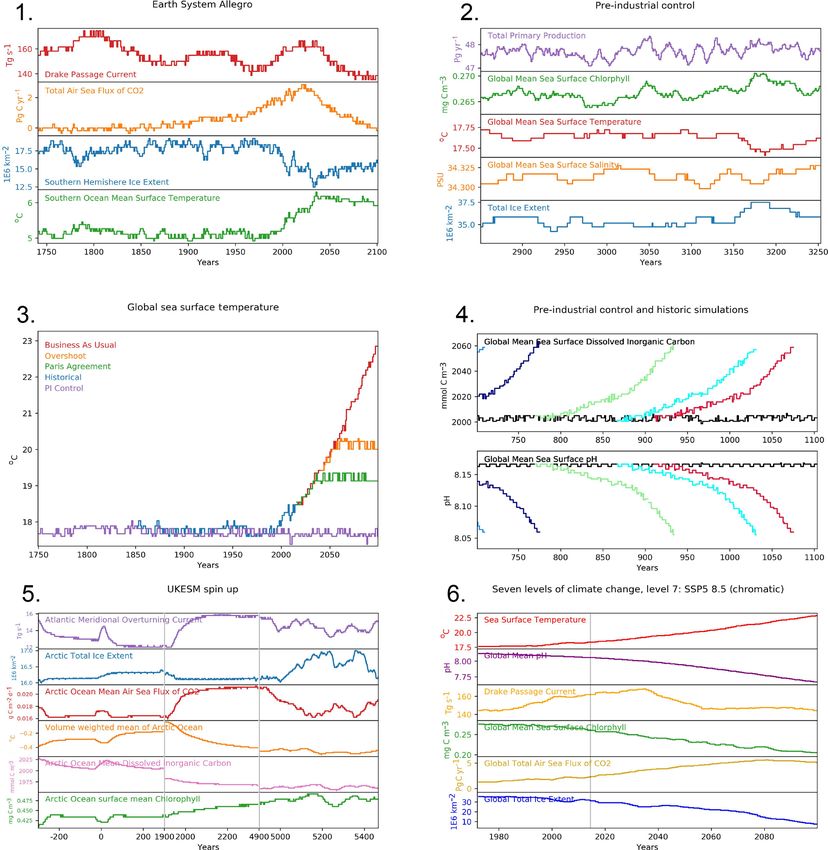
music and the videos. Figure 1 illustrates this process. The velocity is an integer ranging between 1 and 127, where 1 is
initial data are UKESM1 model output files, downloaded di- very quiet and 127 is very loud. The overall tempo of the
rectly from the United Kingdom’s Met Office data storage piece is assigned as a global parameter of the MIDI file in
system (MASS). These native-format UKESM1 data will not units of the number of beats per minute.
be available outside the UKESM collaboration, but selected Each model’s time series data set is converted into a series
model variables have been transformed into a standard for- of consecutive MIDI notes, which together form a track. For
mat and made available on the Earth System Grid Federa- instance, the sea surface temperature (SST) time series could
tion (ESGF) via, for example, https://esgf-index1.ceda.ac.uk/ be converted into a series of MIDI notes in the upper range of
search/cmip6-ceda/, last access: 17 August 2020. the keyboard to form a track. For each track, the time series
The time series data are calculated from the UKESM1 data data are converted into musical notes so that the lowest value
by the BGC-val model evaluation suite (de Mora et al., 2018). in the data set is represented by the lowest note pitch avail-
BGC-val is a software toolkit that was deployed to evaluate able, and the highest value in the data set is represented by
the development and performance of the ocean component of the highest note pitch available. The notes in between are as-
the UKESM1. In all six pieces, we use annual average data signed proportionally by their data value between the lowest
as the time series data. The data sets that were used in this and highest pitched notes. The lowest and highest notes avail-
work are listed in Table 1. able for each track are predefined in the piece’s settings, and
Each time series data set is used to create an individual they are considered an artistic decision. Each track is given
Musical Instrument Digital Interface (MIDI) track composed its own customised pitch range so that the tracks may be at
of a series of MIDI notes. The MIDI protocol is a standard- a lower pitch, higher pitch or have overlapping pitch ranges
ised digital way to convey musical performance information. relative to other tracks in the piece. The ranges of notes avail-
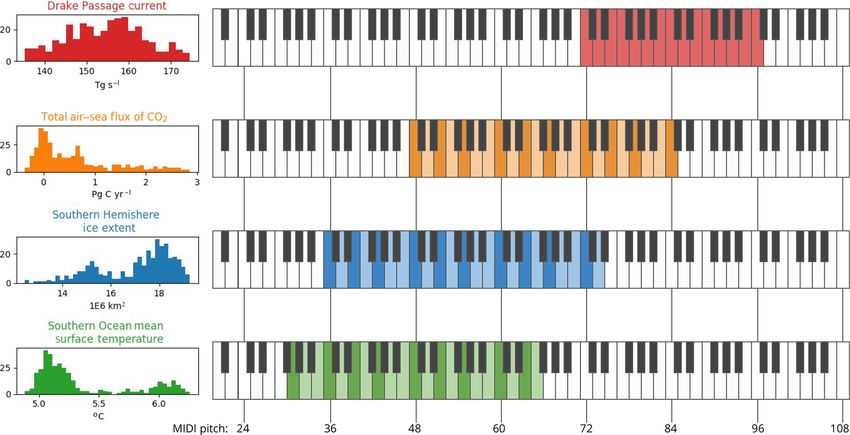
It can be thought of as the instructions that tell a music syn- able for the piece “Earth System Allegro” is shown in Fig. 2.
thesiser how to perform a piece of music (The MIDI Man- In this figure, the four histograms on the left-hand side show
ufacturers Association, 1996). All six pieces shown here are the distributions of the data used in the piece, and the right-
saved as a single MIDI file which contains one or many MIDI hand side includes four standard piano keyboards showing
tracks played simultaneously. Each MIDI track is composed the musical range available in each data set. For instance, the
of a series of MIDI notes. Drake Passage current ranges between 135 and 175 Tg s−1
Each MIDI note is assigned four parameters. The first two in these simulations, and we selected a range between MIDI
parameters are timing (when the note occurs in the song) and pitches 72 and 96. This means that the lowest Drake Passage
duration (the length of time that the note is held). The timing current values (135 Tg s−1 ) would be represented in MIDI
is the number of beats between this note and the beginning of with a pitch of 72, and the highest Drake Passage current
the song. The duration is positive rational number represent-
https://doi.org/10.5194/gc-3-263-2020 Geosci. Commun., 3, 263–278, 2020266 L. de Mora et al.: Earth system music
Figure 1. The computational process used to convert UKESM1 data into a musical piece and an associated video. The boxes with a dark
border represent files and data sets, and the arrows and chevrons represent processes. The blue areas are UKESM1 data and the preprocessing
stages, the green areas show the data and processing stages needed to convert model data into music in the MIDI format, and the orange area
shows the post-processing stages which convert images and MIDI into sheet music and videos.
values (175 Tg s−1 ) would be assigned a MIDI pitch of 96, It then follows that the notes of the C major chord are val-
which is two octaves higher. ues between 0 an 127, where the following condition is true:
These note pitches are then binned into a scale or a chord.
The choice of chord or scale depends on the artistic deci- p ∈ C major0,1,2,...
sions made by the composer. For instance, the C major chord
is composed of the notes C, E and G, which are the zeroth, This can be can be written more simply as follows:
fourth and seventh notes, respectively, in the 12-note chro-
p%12 ∈ C major0 ,
matic scale, starting from C at zero. Figure 3 shows a rep-
resentation of these notes on a standard piano keyboard. The where p represents the pitch value, namely an integer be-
C major in the zeroth octave is composed of the following set tween the minimum and maximum pitches provided in the
of MIDI pitch integers: settings, and the percent sign (%) represents the remainder
C major0 = {0, 4, 7}. (1) operator.
The zeroth octave values for other chords and scales with
the same root note can be calculated from their chromatic
In the 12-tone equal temperament tuning system, the 12 relation with the root note. For instance:
named notes are repeated, and each distance of 12 notes rep-
resents an octave. As shown in Fig. 3, a chord may also C minor0 = {0, 3, 7}
include notes from subsequent octaves. In this figure, the C major70 = {0, 4, 7, 11}
C major chord is highlighted in green, and the zeroth oc-
tave is shown in a darker green than the subsequent octaves. C minor70 = {0, 3, 7, 10}
As such, the C major chord can be formed from any of the ...
following sets of MIDI pitches:
Note that the derivation of these chords and their nomencla-
C major0,1,2,... = {0, 4, 7, 12, 16, 19, 24, 28, 31. . .127}. (2) ture is beyond the scope of this work. For more information
Geosci. Commun., 3, 263–278, 2020 https://doi.org/10.5194/gc-3-263-2020L. de Mora et al.: Earth system music 267
Figure 2. The musical range of each of the data sets used in the “Earth System Allegro”. The four histograms on the left-hand side show
the distributions of the data used in the piece, and the right-hand side shows a standard piano keyboard with the musical range available in
each data set. In this piece, the Drake Passage current, shown in red, is free to vary within a two octave range of the C major scale. The other
three data sets have their own ranges but are limited to the notes in the chord progression, namely C major, G major, A minor and F major.
The dark coloured keys are the notes in C major chord, but the lighter coloured keys show the other notes which are available for the other
chords in the progression. Note that both the C major scale and chord do not include any of the ebony keys on a piano, but these notes could
be used if they were within the available range and appeared in the chord progression used.
For instance:
C major0 = {0, 4, 7}
C# major0 = {0, 4, 7} + 1 = {1, 5, 8}
D major0 = {0, 4, 7} + 2 = {2, 6, 9}
D# major0 = {0, 4, 7} + 3 = {3, 7, 10}
...
Using these methods, we can combinatorially create a list
of all the MIDI pitches in the zeroth octave for all 12 keys for
Figure 3. A depiction of a standard piano keyboard showing the most standard musical chords. From this list, we can convert
names of the notes and the number of these notes in MIDI format. model data into nearly any choice of chord or scale.
The C major chord is highlighted in green, and the zeroth octave is
The conversion from model data to musical pitch is per-
shown in a darker green than the subsequent octaves.
formed using the following method. First, the data are trans-
lated into the pitch scale but kept as a rational number be-
on music theory, please consult an introductory guide to mu- tween the minimum and maximum pitch range assigned by
sic theory such as Schroeder (2002) or Clendinning and Mar- the composer for this data set. As an example, in the piece
vin (2016). “Earth System Allegro” the Drake Passage current was as-
The zeroth octave values for other keys can be included signed a pitch range between 72 and 96, as shown in Fig. 2.
by appending the root note of the scale (C: 0, C#/Db: 1, D: 2, Once the set of possible integer pitches for a given chord or
D#/Eb: 3 and so on) to the relationships in the key of C above. scale has been produced using the methods described above,
the in-scale MIDI pitch with this smallest distance to this ra-
tional number pitch is used. As mentioned earlier, the pitch of
the MIDI notes must be an integer as there is no capacity for
https://doi.org/10.5194/gc-3-263-2020 Geosci. Commun., 3, 263–278, 2020268 L. de Mora et al.: Earth system music
MIDI notes to sit between values on the chromatic scale. The and the number of notes per beat, the musical key and chord
choice of scale is provided in the piece’s settings and is an progression for each track, and the width of the smoothing
artistic choice made by the composer. Furthermore, instead window. The choice of instrument is also another artistic
of using a single chord or scale for a piece, it is also possible choice, although in this work only one instrument was used,
to use a repeating pattern of chords or a chord progression. namely the TiMidity+ piano synthesiser. As a whole, these
The choice of chords, and the order of chords, is different for decisions allow the composer to attempt to define the emo-
each piece. In addition, the number of beats between chord tional context of the final piece. For instance, a fast-paced
changes, and the number of notes per beat, is also assigned piece in a major progression may sound happy and cheer-
in the settings. Furthermore, each track in a given piece may ful to an audience who are used to associating fast-paced
use a different chord progression. songs in major keys with happy and cheerful environments.
The velocity of notes is determined using a similar method It should be mentioned that there are no strict rules governing
to pitch; the time series data are converted into velocities so the emotional context of chords, tempo or instrument, and the
that the lowest value in the data set is the quietest value avail- emotional contexts of harmonies, timbres and tempos differ
able, and the highest value of the data set is the loudest value between cultures. Nevertheless, through exploiting the stan-
available. The notes in between are assigned proportionally dard behaviours of Western musical traditions, the composer
by their data value between the quietest and loudest notes. can attempt to imbue the piece with emotional musical cues
Each track may have its own customised velocity range, such that fit the theme of the piece or the behaviour of the under-
that any given track may be louder or quieter than the other lying climate data.
tracks in a piece. The choice of data set used to determine To create a video, we produced an image for each time step
velocity is provided in the settings. We rarely used the same in each piece. These figures show the data once they have
data set for both pitch and velocity. This is because it results been converted and binned into musical notes using units of
in the high-pitch notes being louder and the low-pitch notes the original data. A still image from each video is shown in
being quieter. Fig. 4. The FFmpeg video editing software (FFmpeg Devel-
After binning the notes into the appropriate scales, all opers, 2017) was used to convert the set of images into a
notes are initially the same duration. If the same pitched note video and to add the MP3 as the soundtrack.
is played successively, then the first note’s duration is ex- The finished videos were uploaded onto the lead author’s
tended and the repeated notes are removed. YouTube channel1 (de Mora, 2019).
A smoothing function may also be applied to the data be-
fore the data set is converted into musical notes. Smoothing
means that it is more likely that the same pitched note will be 4 Works
played successively, so a track with a larger smoothing win-
Six pieces were composed, generated and published using
dow will have fewer notes than a track with a smaller win-
the methods described here. These pieces and their web ad-
dow. From a musical perspective, smoothing slows down the
dresses are below. Note that each of these videos’ last access
piece by replacing fast short notes with longer slower notes.
before this paper was published was 17 August 2020.
Smoothing can also be used to slow down the backing parts
to highlight a faster moving melody. Nearly all the pieces 1. “Earth System Allegro”; https://www.youtube.com/
described here used a smoothing window. watch?v=RxBhLNPH8ls
After applying this method to multiple tracks, they are
saved together in a single MIDI file using the Python 2. “Pre-industrial Vivace”; https://www.youtube.com/
MIDITime library (Corey, 2016). Having created the MIDI watch?v=Hnkvkx4BMk4
file, the piece is performed by the TiMidity++ digital pi-
ano (Izumo and Toivonen, 2004), which converts the MIDI 3. “Ocean Acidification in E minor”; https://www.
format into a digital audio performance in the MP3 format. youtube.com/watch?v=FPeSAA38MjI
In principle, it should be possible to use alternative MIDI
instruments, but for this limited study we exclusively used 4. “Sea Surface Temperature Aria”; https://www.youtube.
the TiMidity++ digital piano. Where possible, the MIDI com/watch?v=SYEncjETkZA
files were converted into sheet music portable document for-
mat (PDF) files using the MuseScore software (MuseScore 5. “Giant Steps Spin Up”; https://www.youtube.com/
BVBA, 2019). However, it is not possible to produce sheet watch?v=fSK6ayp4i4w
music for all six pieces as some have too many MIDI tracks
to be converted to sheet music by this software. 6. “Seven Levels of Climate Change”; https://www.
Each piece has a diverse range of settings and artistic youtube.com/watch?v=2YE9uHBE5OI
choices made by the composer, including the choice of data
sets used to determine pitch and velocity for each track, the 1 See https://www.youtube.com/c/LeedeMora, last access:
pitch and velocity ranges for each track, the piece’s tempo 17 August 2020.
Geosci. Commun., 3, 263–278, 2020 https://doi.org/10.5194/gc-3-263-2020L. de Mora et al.: Earth system music 269 Figure 4. The final frame of each of the six videos. The frames of the videos are shown in the order that they were published. The videos (1), (3), (5) and (6) use a consistent x axis for the duration of the video, but videos (2) and (4) have rolling x axes that change over the course of the video. This means that panels (2) and (4) show only a small part of time range. Panel (5) includes two vertical lines showing the jumps in the spin-up piece. Panel (6) shows a single vertical line for the crossover between the historical and future scenarios. The main goals of the work were to generate music using vace” introduces the concept of a PI control simulation and climate model data and to use music to illustrate some stan- highlights how an emotional connection can be made be- dard practices in Earth system modelling that might not be tween the model output and the sonification of the data. The widely known outside our community. Beyond these broader goal of the “Sea Surface Temperature Aria” is to demon- goals, each piece had its own unique goal; for example, to strate the range of behaviours of the future climate projec- demonstrate the principles of sonification using UKESM1 tions. “Ocean Acidification in E minor” aims to show the data in the “Earth System Allegro”. The “Pre-industrial Vi- impact of rising atmospheric CO2 on ocean acidification and https://doi.org/10.5194/gc-3-263-2020 Geosci. Commun., 3, 263–278, 2020
270                                                                                       L. de Mora et al.: Earth system music

also to illustrate how historical runs are branched from the       the first, fifth, sixth and fourth chords in the root of C major.
PI control. The “Giant Steps Spin Up” shows the process of         This progression is strikingly popular and may be heard in
spinning up the marine component of the UKESM1, and fi-            songs such as “Let it be” by the Beatles, “No woman no cry”
nally, the “Seven Levels of Climate Change” aims to use the        by Bob Marley and the Whalers, “With or without you” by
musical principles of jazz harmonisation to distinguish the        U2, “I’m yours” by Jason Mraz and “Africa” by Toto, among
full set of UKESM1’s future scenario simulations.                  many others. By choosing such a common progression, we
   These six pieces are summarised in Fig. 4 and Table 1.          were aiming to introduce the concept of musification of data
Figure 4 shows the final frame of each of the pieces, and          using familiar-sounding music and to avoid alienating the au-
Table 1 shows the summary of each of the videos, including         dience.
the publication date and duration, and lists the experiments
and data sets used to generate the piece.                          4.2   “Pre-industrial Vivace”

4.1   “Earth System Allegro”
                                                                   The “Pre-industrial Vivace” is a fast-paced piece in C ma-
                                                                   jor, showing various metrics of the behaviour of the global
The “Earth System Allegro” is a relatively fast-paced piece        ocean in the PI control run. The PI control run is a long-
in C major, showing some important metrics of the Southern         term simulation of the Earth’s climate without the impact of
Ocean in the recent past and projected into the future with        the industrial revolution or any of the subsequent human im-
the shared socioeconomic pathway (SSP) scenario, SSP1 1.9.         pact on climate. At the time that the piece was created, there
The SSP1 1.9 projection is the future scenario in which the        were approximately 1400 simulated years. We use the con-
anthropogenic impact on the climate is the smallest. The           trol run as the starting point for historical simulations but also
C major scale is composed of only natural notes (no sharp          to compare the difference between human-influenced simula-
or flat notes), making it one of the first chords that people      tions and simulations of the ocean without any anthropogenic
encounter when learning music. In addition, major chords           impact.
and scales like C major typically sound happy. Christian              The final frame of the “Pre-industrial Vivace” video is
Schubart’s “Ideen zu einer Aesthetik der Tonkunst” (1806)          shown in panel (2) of Fig. 4. The top pane of this video shows
describes C major as “Completely pure. Its character is: in-       the global marine primary production in purple. The primary
nocence, simplicity, naivety, children’s talk” (Schubart and       production is a measure of how much marine phytoplankton
DuBois, 1983) Through choosing C major and an upbeat               is growing. Similarly, the second pane shows the global ma-
tempo and data from the best possible climate scenario             rine surface chlorophyll concentration in green; this line rises
(SSP1 1.9), we aimed to start the project with a piece with a      and falls alongside the primary production in most cases. The
sense of optimism about the future climate and to introduce        third and fourth panes show the global mean sea surface tem-
the principles of musification of the UKESM1 time series           perature and sea surface salinity (SSS) in red and orange.
data.                                                              The fifth pane shows the global total ice extent. These five
   The Drake Passage current, shown in panel (1) of Fig. 4,        fields are an overview of the behaviour of the pristine natu-
is a measure of the strongest current in the ocean, namely the     ral ocean of our Earth system model. There is no significant
Antarctic Circumpolar current. This is the current that flows      drift, and there is no long-term trend in any of these fields.
eastwards around Antarctica. The second data set, shown            However, there is significant natural variability operating at
here in orange, is the global total air to sea flux of CO2 .       decadal and millennial scales.
This field shows the global total atmospheric carbon diox-            As with the “Earth System Allegro”, “Pre-industrial Vi-
ide that is absorbed into the ocean each year. Even under          vace” uses the familiar C major scale but adds a slight vari-
SSP1 1.9, UKESM1 predicts that this value would rise from          ation to the chord progression. The first half of the progres-
around zero during the pre-industrial period to a maximum          sion is C major, G major, A minor and F major, but it follows
of approximately 2 Pg of carbon per year around the year           with a common variant of this progression, namely C major,
2030, followed by a return to zero at the end of the century.      D minor, E minor and F major. Through using the lively vi-
The third field is the sea ice extent of the Southern Hemi-        vace tempo and a familiar chord progression in a major key,
sphere, shown in blue. This is the total area of the ocean in      this piece aims to use musification to link the PI control sim-
the Southern Hemisphere which has more that 15 % ice cov-          ulation with a sense of happiness and ease. The lively, fast
erage per grid cell of our model. The fourth field is the South-   and jovial tone of the piece should match the pre-industrial
ern Ocean mean surface temperature, shown in green, which          environment, which is free running and uninhibited by an-
rises slightly from approximately 5 ◦ C in the pre-industrial      thropogenic pollution.
period up to a maximum of 6 ◦ C. The ranges of each data set
are illustrated in Fig. 2.                                         4.3   “Sea Surface Temperature Aria”
   In this piece, the Drake Passage current is set to the C ma-
jor scale, but the other three parts modulate between the          The “Sea Surface Temperature Aria” demonstrates the
C major, G major, A minor and F major chords. These are            change in sea surface temperature in the PI control run, the

Geosci. Commun., 3, 263–278, 2020                                                        https://doi.org/10.5194/gc-3-263-2020
Table 1. The video publication details, including the publication date, the duration, the Coupled Model Intercomparison Project (CMIP) experiment names and the data sets used. Note:
DIC – dissolved inorganic carbon; PI control – pre-industrial control; SSP – shared socioeconomic pathway; SST – sea surface temperature. Note that each of these videos’ last access
before this paper was published was 17 August 2020.
Video title Publication date Duration Experiments Data sets
(dd-mm-yyyy) (mm:ss)
L. de Mora et al.: Earth system music
“Earth System Allegro” 21-08-2019 01:02 Historical, SSP1 2.5
https://doi.org/10.5194/gc-3-263-2020
Drake Passage current, total air–sea flux of CO2 ,
(https://www.youtube.com/ Southern Hemisphere ice extent and Southern Ocean SST
watch?v=RxBhLNPH8ls)
“Pre-industrial Vivace” 21-08-2019 02:27 PI control Total primary production, global mean sea surface,
(https://www.youtube.com/ chlorophyll, SST, SSS, total ice extent
watch?v=Hnkvkx4BMk4)
“Ocean Acidification 22-08-2019 01:56 PI control, historical Global mean surface DIC
in E minor”
(https://www.youtube.com/ Global mean surface mean pH
watch?v=FPeSAA38MjI)
“Sea Surface 02-09-2019 01:17 PI control, historical, Global mean SST
Temperature Aria” SSP1 1.9, SSP5 3.4 OS, SSP5 8.5
(https://www.youtube.com/
watch?v=SYEncjETkZA)
“Giant Steps Spin Up” 13-09-2019 02:52 Spin up Atlantic meridional overturning current, Arctic ice extent,
(https://www.youtube.com/ Arctic mean air–sea flux of CO2 , volume-weighted mean
watch?v=fSK6ayp4i4w) temperament of the Arctic Ocean, global surface mean DIC,
mean surface chlorophyll in the arctic
“Seven Levels of 14-10-2019 02:55 PI control, historical, SSP1 1.9, Global mean SST, pH, Drake Passage current, global mean
Climate Change” SSP1 2.6, SSP4 3.4, SSP5 3.4 – surface chlorophyll, global total air–sea flux of CO2 , global
(https://www.youtube.com/ overshoot, SSP2 4.5, total ice extent
watch?v=2YE9uHBE5OI) SSP3 7.0, SSP5 8.5
Geosci. Commun., 3, 263–278, 2020
271272 L. de Mora et al.: Earth system music
historical scenario and under three future climate projection bar blues can be heard in songs such as “Johnny B. Goode”
scenarios, as shown in panel (3) of Fig. 4. The first scenario by Chuck Berry, “Hound dog” by Elvis Presley, “I got you
is the “business as usual” scenario (SSP5 8.5; shown in red) (I feel Good)” by James Brown, “Sweet home Chicago” by
in which human carbon emissions continue without mitiga- Robert Johnson or “Rock and roll” by Led Zeppelin. In the
tion. The second scenario is an “overshoot” scenario, namely context of Earth system music, the 12 bar pattern with its
an SSP5 3.4-overshoot, in which emissions continue to grow opening set of four bars, then two sets of two bars and end-
but then drop rapidly in the middle of the 21st century, as ing with four sets of one bar between key changes drives the
shown in orange. The third scenario is SSP1 1.9, labelled as song forward before starting again slowly. This behaviour is
the “Paris Agreement” scenario and shown in green, in which thematically similar to the behaviour of the ocean acidifica-
carbon emissions drop rapidly from the present day. The goal tion in UKESM1 historical simulation, in which the bulk of
of this piece is to demonstrate the range of differences be- the acidification occurs at the end of each historical period.
tween some of the SSP scenarios on sea surface temperature. This video highlights that the marine carbon system has
The PI control run and much of the historical scenario been heavily impacted over the historical period. In the PI
data are relatively constant. However, they start to diverge control runs, both the pH and the DIC are very stable. How-
in the 1950s. In the future scenarios, the three projects all ever, in all historical simulations with rising atmospheric
behave similarly until the 2030s; then the SSP1 1.9 scenario CO2 , the DIC concentration rises and the pH falls. The pro-
branches off and maintains a relatively constant global mean cess of ocean acidification is relatively simple and well un-
sea surface temperature. The SSP5 3.4 scenario’s SST con- derstood (Caldeira and Wickett, 2003; Orr et al., 2005). The
tinues to grow until the year 2050, while the SSP5 8.5 sce- atmospheric CO2 is absorbed from the air into the ocean
nario’s SST grows until the end of the simulation. surface, which releases hydrogen ions into the ocean, mak-
Musically, this piece is consistently in the scale of A mi- ing the ocean more acidic. The concentration of DIC in the
nor harmonic, with no modulating chord progression. The sea surface is closely linked with the concentration of at-
minor harmonic scale is a somewhat artificial scale in that it mospheric CO2 , and it rises over the historic period. This
augments seventh note of the natural minor scale. The aug- behaviour was observed in every single UKESM1 historical
mented seventh means that there is a minor third between the simulation. This video also illustrates an important part of the
sixth and seventh note, making it sound uneasy and sad (at methodology used to produce models of the climate that may
least to the author’s ears). An aria is a self-contained piece not be widely known outside our community. When we pro-
for one voice, normally within a larger work. In this case, duce models of the Earth system, we use a range of points of
the name “aria” is used to highlight that only one data set, the PI control as the initial conditions for the historical sim-
namely the sea surface temperature, participates in the piece. ulations. All the historical simulations have slightly different
This piece starts relatively low and slow, then grows higher starting points, and evolve from these different initial condi-
and louder as the future scenarios are added to the piece. The tions, which give us more confidence that the results of our
unchanging minor harmonic chord, slow tempo and pitch projections are due to changes since the pre-industrial period
range were chosen to elicit a sense of dread and discord as instead of simply a consequence of the initial conditions. In
the piece progresses to the catastrophic SSP5 8.5 scenario at this figure, the historical simulations are shown where they
the end of the 21st century. branch from the PI control run instead of using the “real”
time as the x axis.
4.4 “Ocean acidification in E minor”
4.5 “Giant Steps Spin Up”
“Ocean acidification in Eminor ” demonstrates the standard
modelling practice of branching historical simulations from This piece combines the spin up of the United Kingdom
the PI control run and the impact of rising anthropogenic car- Earth System Model with the chord progression of John
bon on the ocean carbon cycle. The final frame of this video Coltrane’s “Giant steps” (Coltrane, 1960). The spin up is
is shown in panel (4) of Fig. 4. The top pane shows the global the process of running the model from a set of initial
mean dissolved inorganic carbon (DIC) concentration in the conditions to a near-steady-state climate. When a model
surface of the ocean, and the lower pane shows the global reaches a steady state, this means that there is no signifi-
mean sea surface pH. In both panes, the PI control run data cant trend or drift in the mean behaviour of several key met-
are shown as a black line, and the coloured lines represent rics. For instance, as part of the Coupled Climate Carbon Cy-
the 15 historical simulations. cle Model Intercomparison Project (C4MIP) protocol, Jones
This piece uses a repeating “12 bar blues” structure in et al. (2016) suggest a drift criterion of less than 10 Pg of car-
E minor and a relatively fast tempo. This chord progression bon per century in the absolute value of the flux of CO2 from
is an exceptionally common progression, especially in blues, the atmosphere to the ocean. In practical terms, the ocean
jazz and early rock and roll. It is composed of four bars of model is considered to be spun up when the long-term aver-
the E minor, two bars of A minor, two bars of E minor, then age of the air–sea flux of carbon is consistently between −0.1
one bar of B minor, A minor, E minor and B minor. The 12 and 0.1 Pg of carbon per year.
Geosci. Commun., 3, 263–278, 2020 https://doi.org/10.5194/gc-3-263-2020L. de Mora et al.: Earth system music 273
The spin up is a crucial part of model development. With- repeating atmospheric forcing data set used to spin up the
out spinning up, the historical ocean model would still be ocean model.
equilibrating with the atmosphere. It would be much more
difficult to separate the trends in the historical and future 4.6 “Seven Levels of Climate Change”
scenarios from the underlying trend of a model still trying
to equilibrate. Note that while a steady-state model does not This piece is based on a YouTube video by Adam Neely,
have any significant long-term trends or drifts, it can still called “The 7 levels of jazz harmony” (Neely, 2019). In that
have short-term variability. This short-term variability can be video, Neely demonstrates seven increasingly complex lev-
seen in the pre-industrial simulation in the “Pre-industrial Vi- els of jazz harmony by re-harmonising a line of the cho-
vace” piece. It can take a model thousands of years of simu- rus of Lizzo’s song “Juice”. We have repeated Neely’s re-
lations for the ocean to reach a steady state. In our case, the harmonisation of “Juice” here, such that each successive
spin up ran for approximately 5000 simulated years before level’s note choice is informed by Earth system simula-
the spun up drift criterion was met (Yool et al., 2020). tions, with increasing levels of emissions and stronger an-
The UKESM1 spin up was composed of several phases thropogenic climate change.
in succession. The first stage was a fully coupled run using At the time of writing, UKESM1 had produced simula-
an early version of UKESM1. Then, an ocean-only run was tions of seven future scenarios. The seven scenarios of cli-
started using a 30 year repeating atmospheric forcing data mate change and their associated jazz harmony are as fol-
set. The beginning of this part of the run is considered to lows:
be the beginning of the spin up, and the time axis is set to
– Level 0: PI control – original harmony
zero at the start of this run. This is because the early version
of UKESM1 did not include a carbon system in the ocean. – Level 1: SSP1 1.9 – four note chords
After about 1900 years of simulating the ocean with the re-
peating atmospheric forcing data set, we had found that some – Level 2: SSP1 2.6 – tritone substitution
changes were needed to the physical model. At this point, we
– Level 3: SSP4 3.4 – tertiary harmony extension
initialised a new simulation from the final year of the previ-
ous stage and changed the atmospheric forcing. This second – Level 4: SSP5 3.4 (overshoot) – pedal point
ocean-only simulation ran until the year 4900. At the point,
we finished the spin up with a few hundred years of fully – Level 5: SSP2 4.5 – non-functional harmony
coupled UKESM1 with ocean, land, sea ice and atmosphere
– Level 6: SSP3 7.0 – liberated dissonance
models. Due to the slow and repetitive native of the ocean-
only spin up, several centuries of data were omitted. These – Level 7: SSP5 8.5 – fully chromatic
are marked as grey vertical lines in the video and panel (5) of
Fig. 4. Note that we were not able to reproduce Neely’s seventh
The piece is composed of several important metrics of the level, namely intonalism or xenharmony. In this level, the in-
spin up in the ocean, such as the Atlantic meridional over- tonation of the notes are changed depending on the underly-
turning current (purple), Arctic ocean total ice extent (blue), ing melody. Unfortunately, the MIDITime Python interface
the global air–sea flux of CO2 (red), the volume-weighted for MIDI has not yet reached such a level of sophistication.
mean temperature of the Arctic ocean (orange), the surface Instead, we simply allow all possible values of the 12-note
mean DIC in the Arctic Ocean (pink) and the surface mean chromatic scale.
chlorophyll concentration in the Arctic ocean (green). The data sets used in this piece are a set of global-scale
The music is based on the chord progression from the jazz metrics that show the bulk properties of the model under
standard, John Coltrane’s “Giant steps”, although the musical the future climate change scenarios. They include the global
progression was slowed to one chord change per four beats mean SST (red), the global mean surface pH (purple), the
instead of a change at every beat. This change occurred as an Drake Passage current (yellow), the global mean surface
accident, but we found that the full-speed version sounded chlorophyll concentration (green), the global total air to sea
very chaotic, so the slowed version was published instead. flux to CO2 (gold) and the global total ice extent (blue). As
This piece was chosen because it has a certain notoriety due the piece progresses through the seven levels, the anthro-
to the difficulty for musicians to improvise over the rapid pogenic climate change in the model becomes more extreme,
chord changes. In addition, “Giant steps” was the first new matching the increasingly esoteric harmonies of the music.
composition to feature Coltrane changes. Coltrane changes
are a complex cyclical harmonic progression which form a 5 Limitations and potential extensions
musical framework for jazz improvisation. We hoped that the
complexity of the Earth system model is reflected in the com- We have successfully demonstrated that it is possible to gen-
plexity of the harmonic structure of the piece. The cyclical erate music using data from the UK’s Earth System Model.
relationship of the Coltrane changes also reflects the 30 year We have also shown that we can illustrate some standard
https://doi.org/10.5194/gc-3-263-2020 Geosci. Commun., 3, 263–278, 2020274 L. de Mora et al.: Earth system music practices in Earth system modelling using music. Within the If additional pieces were made, there are several potential framework of this pilot study, we must also raise some limi- ways that the methodology used to create them could be im- tations and suggest some possible extensions for future ver- proved relative to the methods used to create the initial set sions of this work. of videos. In future versions of this work, it should be pos- A significant omission from this study is the measurement sible to use the ESMValTool (Righi et al., 2019) to produce of the impact, the reach or the engagement of these works. the time series data instead of BGC-val. This would make We did not test whether the audience was composed of the production of the time series more easily repeatable but laypeople or experts. We did not investigate whether the au- would also make it easier for pieces to be composed using dience learnt anything about Earth system modelling through data available in the CMIP5 and CMIP6 coupled model inter- these series of videos. We did not monitor the audience re- comparison projects. This broadens the scope of the data by actions or interpretations of the music. Future extensions of allowing other models, other model domains, including the this project should include a survey of the audience to inves- atmosphere and the land surface, and even observational data tigate their backgrounds and demographics, what they learnt sets. For instance, we could make a multi-model intercom- about Earth system models, and their overall impressions of parison piece or a piece based on the atmospheric, terrestrial the pieces. This could take the form of an online survey as- and ocean components of the same model. In addition, us- sociated with each video or a discussion with the audience at ing ESMValTool would also make it more straightforward to a live performance. distribute the source code that was used to make these pieces. In addition, in this work, we make no effort to monitor or In the reflections on auditory graphics, Flowers (2005) describe the reach of the YouTube videos, track comments, lists several “Things that work” and “Approaches that do not subscriptions or the source of the views. While some tools work”. From the list of things that work, we included four are available for monitoring the number of videos within of the five methods that worked: pitch coding of numeric YouTube’s content creator toolkit, YouTube Studio (Google, data, the exploitation of temporal resolution of human audi- 2019), a preliminary investigation found that it was not pos- tion, manipulating loudness changes and using time as time. sible to use these tools alone to create a sufficiently detailed We were not able to include the selection of distinct timbres analyses of the impact, reach or dissemination of these music to minimise stream confusion. From the list of approaches creation methods. YouTube Studio currently includes some that do not work, we successfully avoided several of the pit- demographic details, including gender, country of origin, falls, notably pitch mapping to continuous variables and us- viewership age, and traffic source, but it is not sufficient for ing loudness changes to represent an important continuous an audience survey. This toolkit was built to help content cre- variable. However, we did include one of the approaches that ators monitor and build their audience and to monetise videos Flowers did not recommend: we simultaneously plotted sev- using advertisements. It is not fit for the purpose of scientific eral variables with similar pitches and timbres. However, it is engagement monitoring. For instance, it was not possible to worth noting that maximising the clarity of the sonification is use YouTube Studio to determine the expertise of the audi- the goal of Flowers (2005), but our focus was to produce and ence, their thoughts on climate change, whether they read the disseminate some relatively listenable pieces of music using video description section or whether they understood the de- UKESM1 data. scription. Some of these features could be added to YouTube The two suggestions by Flowers (2005) that we failed to by Google, but many of them would require the audience sur- address were both related to using the same timbre digital pi- vey described above. ano synthesiser for all data. Due to the technical limitations Our videos only include the music and a visualisation of of using TiMidity++, we were not able to vary the instru- the data; they do not include any description about how the ments used, and thus there was very little variability in terms music was generated or the Earth system modelling meth- of the timbres. These pieces were all performed by the same ods used to create the underlying data. The explanations of instrument, a solo piano, which limits the musical diversity the science and musification methodologies are given in a of the set of pieces. In addition, each data set in a given piece description below the video. Furthermore, viewers must ex- was performed by the same instrument, making it difficult pand this box by clicking the “show more” button. Using the to distinguish the different data sets being performed simul- tools provided in YouTube studio, it is not currently possible taneously. Further extensions of this work could use a fully to determine whether the viewers have expanded, read or un- featured digital audio workstation to access a range of digital derstood the description section. When we have shown these instruments beyond the digital piano, such as a string quartet, videos to audiences at scientific meetings and conferences, a horn and woodwind section, a full digital orchestra, electric it has always been associated with a brief explanation of the guitar and bass, percussive instruments, or electronic synthe- methods. In future, this explanatory preface to the work could sised instruments. This would comply with the suggestions be included in the video itself, or as a separate video, in ad- listed in Flowers (2005), allowing the individual data sets to dition to the text below the video in the description section. stand out musically from each other in an individual piece, This would likely increase the audience’s understanding of but would also lead to a much more diverse set of musical our music-generation process. pieces. Geosci. Commun., 3, 263–278, 2020 https://doi.org/10.5194/gc-3-263-2020
L. de Mora et al.: Earth system music                                                                                         275

   From a musical perspective, there are many ways to im-             YouTube videos are typically shown in the suggestions
prove the performances of the pieces for future versions of        queue with a thumbnail image and the video title. The thumb-
this work. As raised in the comments from social media, a          nail is the graphic placeholder that shows the video while it
human pianist would be able to add a warmth to the perfor-         is not playing on YouTube as a suggested video or in Face-
mance that is beyond the abilities of MIDI interpreters. A         book or Twitter feeds. The thumbnail is how viewers first
recording of a human performance could also add the hidden         encounter the video, and it is a crucial part of attracting an
artefacts of a live recording, such as room noise, stereo ef-      audience. There are lots of guides helping one to create bet-
fects and natural reverb. On the other hand, due to the nature     ter thumbnails (Kjellberg and PewDiePie, 2017; Video Influ-
of the process used to generate these pieces, it may not be        encers, 2016; Myers, 2019). Future works should attempt to
possible for a single human to perform several of the pieces       optimise the video thumbnail to attract a wider audience.
due to the speed, complexity, number of simultaneous notes            While we did not investigate the reach or dissemination of
or the range of these pieces. Alternatively, it may be possi-      these pieces in this work, if the goal of future projects was to
ble to “humanise” the MIDI by making subtle changes to the         increase the online audience size then it might be possible to
timing and velocities of the MIDI notes. This is a recording       reach a wider audience using a press release, a public screen-
technique that can take a synthesised, perfectly timed beat        ing of the videos, a scheduled publication date or through a
and make it sound like it is being played by a human. It does      collaboration with other musicians or YouTube content cre-
this by moving the individual notes slightly before or after       ators. It may also be possible to host a live concert, make a
the beat, and adding subtle variations in the velocity (Walden,    live recording or broadcast a YouTube live stream. It is not
2017). Also, TiMidity++ uses the same piano sample for             fully understood how a video can go viral, but it has been
each pitch. This means that when two tracks of a piece play        shown that view counts can rise exponentially when a single
the same pitch at the same time, exactly the same sample           person or organisation with a large audience shares a video
is played twice simultaneously. These two identical sample         (West, 2011; Jiang et al., 2014). Improvements to the music,
sound waves are added constructively, and the note jumps           the video, the description and the thumbnail make it more
out much louder than it would if a human played the part. A        likely for such an influencer with large audience to like, share
fully featured digital piano or a human performance would          or retweet a piece, which could result in a significant increase
remove these loud jumps but also be able to add more nuance        in the audience size and view count. The videos in this work
and warmth to the performance. Finally, the published pieces       were posted online in an ad hoc fashion as soon as they were
had no mastering or post-production. Even a basic mastering        finished. To maximise the number of views, experts have rec-
session by a professional sound engineer would likely im-          ommended consistent, scheduled in advance, weekly videos,
prove the overall quality of the sound of these pieces.            and it has been advised to publish them late in the week in
   In terms of the selection of chords progression, tempo and      the afternoons (Cox, 2017; Think Media, 2017). Finally, it
rhythms, it may be possible to target specific audiences using     should be possible to increase the reach of this work through
music based on popular artists or genres. For instance, the        paid advertising on YouTube and other social media plat-
reach of a piece might be increased by responding to viral         forms. This would place the videos higher in the suggested
videos or by basing a work on a popular song.                      video rankings and on the discovery queues.
   In these works, we have focused on reproducing Western
music, both traditional and modern, in order to connect each
piece with the associated emotional musical cues. Alterna-         6   Conclusions
tively, there is a significant diversity in traditional and mod-
ern styles of music from other regions around the world; a         In this work, we took data from the first United Kingdom
much wider range of rhythms, timbres, styles and emotional         Earth System Model and converted it into six musical pieces
cues could be exploited in future extensions of this work.         and videos. These pieces covered the core principles of cli-
   With regards to the visual aspect of these videos, it should    mate modelling or ocean modelling, namely PI control runs,
be straightforward to improve the quality of the graphics          the spin-up process, multiple future scenarios, the Drake Pas-
used. The current videos only show a simple scalar field as        sage current, the air–sea flux of CO2 and the Atlantic merid-
it develops over time. They could be improved by adding            ional overturning circulation. While limited to a single instru-
animated global maps of the model, interviews or live per-         ment, namely the synthesised piano, they included a range of
formances to the video. It may also be a positive addition         musical styles, including classical, jazz, blues and contem-
to preface the videos with a brief explanation of the project      porary styles.
and the methods deployed. On the technical side, there may            While the wider public are likely to be familiar with cli-
also be some visual glitches and artefacts which arise due to      mate change, they are less likely to be familiar with our com-
YouTube’s compression or streaming algorithms. A different         munity’s methods. In fact, many standard tools in the arsenal
streaming service or alternative video making software might       of climate modellers may not be widely appreciated outside
help remove these glitches.                                        our small community, even within the scientific community.
                                                                   These six musical pieces open the door on a new, exciting

https://doi.org/10.5194/gc-3-263-2020                                                    Geosci. Commun., 3, 263–278, 2020
You can also read