Systematic identification of external influences in multi-year microseismic recordings using convolutional neural networks
←
→
Page content transcription
If your browser does not render page correctly, please read the page content below
Earth Surf. Dynam., 7, 171–190, 2019
https://doi.org/10.5194/esurf-7-171-2019
© Author(s) 2019. This work is distributed under
the Creative Commons Attribution 4.0 License.

          Systematic identification of external influences in
        multi-year microseismic recordings using convolutional
                            neural networks
                          Matthias Meyer1 , Samuel Weber2,1 , Jan Beutel1 , and Lothar Thiele1
                    1 Computer   Engineering and Networks Laboratory, ETH Zurich, Zurich, Switzerland
                           2 Department  of Geography, University of Zurich, Zurich, Switzerland
                            Correspondence: Matthias Meyer (matthias.meyer@tik.ee.ethz.ch)

                                   Received: 26 July 2018 – Discussion started: 6 August 2018
                     Revised: 16 November 2018 – Accepted: 17 December 2018 – Published: 4 February 2019

      Abstract. Passive monitoring of ground motion can be used for geophysical process analysis and natural haz-
      ard assessment. Detecting events in microseismic signals can provide responsive insights into active geophysical
      processes. However, in the raw signals, microseismic events are superimposed by external influences, for exam-
      ple, anthropogenic or natural noise sources that distort analysis results. In order to be able to perform event-based
      geophysical analysis with such microseismic data records, it is imperative that negative influence factors can be
      systematically and efficiently identified, quantified and taken into account. Current identification methods (man-
      ual and automatic) are subject to variable quality, inconsistencies or human errors. Moreover, manual methods
      suffer from their inability to scale to increasing data volumes, an important property when dealing with very
      large data volumes as in the case of long-term monitoring.
         In this work, we present a systematic strategy to identify a multitude of external influence sources, characterize
      and quantify their impact and develop methods for automated identification in microseismic signals. We apply
      the strategy developed to a real-world, multi-sensor, multi-year microseismic monitoring experiment performed
      at the Matterhorn Hörnligrat (Switzerland). We develop and present an approach based on convolutional neural
      networks for microseismic data to detect external influences originating in mountaineers, a major unwanted
      influence, with an error rate of less than 1 %, 3 times lower than comparable algorithms. Moreover, we present
      an ensemble classifier for the same task, obtaining an error rate of 0.79 % and an F1 score of 0.9383 by jointly
      using time-lapse image and microseismic data on an annotated subset of the monitoring data. Applying these
      classifiers to the whole experimental dataset reveals that approximately one-fourth of events detected by an event
      detector without such a preprocessing step are not due to seismic activity but due to anthropogenic influences
      and that time periods with mountaineer activity have a 9 times higher event rate. Due to these findings, we argue
      that a systematic identification of external influences using a semi-automated approach and machine learning
      techniques as presented in this paper is a prerequisite for the qualitative and quantitative analysis of long-term
      monitoring experiments.

Published by Copernicus Publications on behalf of the European Geosciences Union.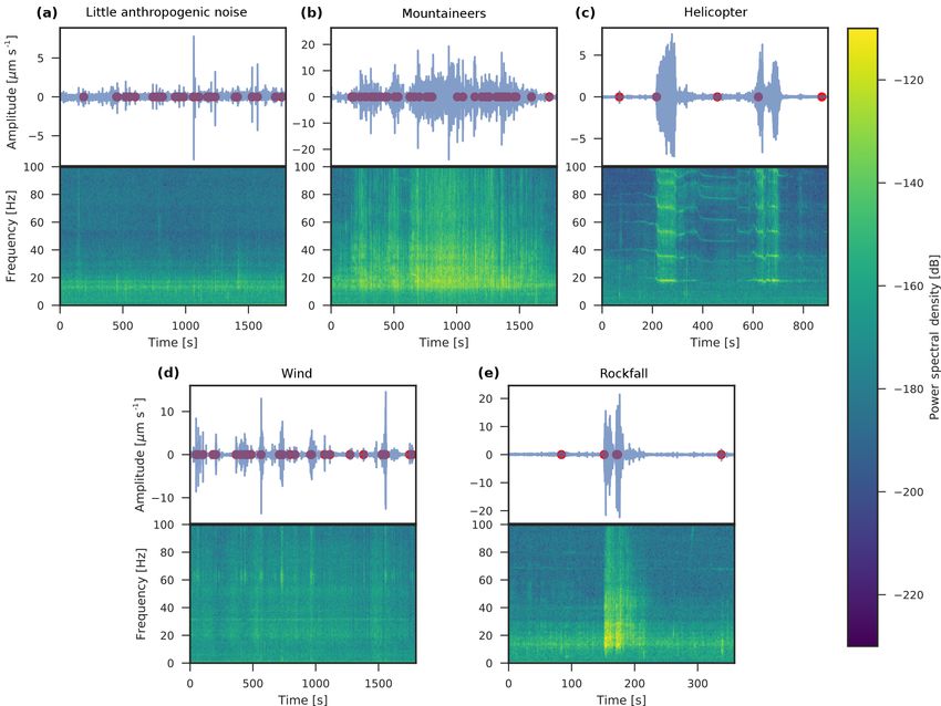
172                  M. Meyer et al.: Systematic identification of external influences in multi-year microseismic recordings

1   Introduction                                                   on the signals recorded. As a conclusion, it is a requirement
                                                                   that external influences can be taken into account with an
Passive monitoring of elastic waves, generated by the rapid        automated workflow, including preprocessing, cleaning and
release of energy within a material (Hardy, 2003) is a non-        analysis of microseismic data.
destructive analysis technique allowing a wide range of ap-           A frequently used example of an event detection mecha-
plications in material sciences (Labuz et al., 2001), engineer-    nism is an event detector called STA/LTA that is based on
ing (Grosse, 2008) and natural hazard mitigation (Michlmayr        the ratio of short-term average to long-term average (Allen,
et al., 2012) with recently increasing interest into investiga-    1978). Due to its simplicity, this event detector is commonly
tions of various processes in rock slopes (Amitrano et al.,        used to assess seismic activity by calculating the number of
2010; Occhiena et al., 2012). Passive monitoring techniques        triggering events per time interval for a time period of in-
may be broadly divided into three categories, characterized        terest (Withers et al., 1998; Amitrano et al., 2005; Senfaute
by the number of stations (single vs. array), the duration of      et al., 2009). It is often used in the analysis of unstable slopes
recording (snapshot vs. monitoring) and the type of analysis       (Colombero et al., 2018; Levy et al., 2011) and is available
(continuous vs. event-based). On the one hand, continuous          integrated into many commercially available digitizers and
methods such as the analysis of ambient seismic vibrations         data loggers (Geometrics, 2018). With respect to unwanted
can provide information on internal structure of a rock slope      signal components, STA/LTA has also been used to detect
(Burjánek et al., 2012; Gischig et al., 2015; Weber et al.,        external influence factors such as footsteps (Anchal et al.,
2018a). On the other hand, event-based methods such as the         2018) but due to its inherent simplicity, it cannot reliably
detection of microseismic events (which are the focus of this      discriminate geophysical seismic activity from external (un-
study) can give immediate insight into active processes, such      wanted) influence factors such as noise from humans and nat-
as local irreversible (non-elastic) deformation occurring due      ural sources like wind, rain or hail without manually super-
to the mechanical loading of rocks (Grosse and Ohtsu, 2008).       vising and intervening in the detection process on a case-by-
However, for the reliable detection of events irrespective of      case basis. As a result, the blind application of STA/LTA will
the detection method, the signal source of concern has to be       inevitably lead to the false estimation of relevant geophysical
distinguishable from noise, for example, background seis-          processes if significant external influences, such as wind, are
micity or other source types. This discrimination is a com-        present (Allen, 1978).
mon and major problem for analyzing microseismic data.                There exist several algorithmic approaches to mitigate
   In general, event-based geoscientific investigations focus      the problem of external influences by increasing the selec-
on events originating from geophysical sources such as me-         tivity of event detection. These include unsupervised algo-
chanical damage, rupture or fracture in soil, rock and/or ice.     rithms such as auto-correlation (Brown et al., 2008; Aguiar
These sources originate, for example, in thermal stresses,         and Beroza, 2014; Yoon et al., 2015), but these are ei-
pressure variations or earthquakes (Amitrano et al., 2012).        ther computationally complex or do not perform well for
However, non-geophysical sources can trigger events as well:       low signal-to-noise ratios. Supervised methods can find
(i) anthropogenic influences such as helicopter or moun-           events in signals with low signal-to-noise ratio. For exam-
taineers (Eibl et al., 2017; van Herwijnen and Schweizer,          ple, template-matching approaches such as cross-correlation
2011; Weber et al., 2018b) and (ii) environmental influ-           methods (Gibbons and Ringdal, 2006) use event examples
ences/disturbances, such as wind or rain (Amitrano et al.,         to find similar events, failing if events differ significantly
2010). One way to account for such external influences is to       in “shape” or if the transmission medium is very inhomo-
manually identify their sources in the recordings (van Herwi-      geneous (Weber et al., 2018b). The most recent supervised
jnen and Schweizer, 2011). This procedure, however, is not         methods are based on machine learning techniques (Reynen
feasible for autonomous monitoring because manual identifi-        and Audet, 2017; Olivier et al., 2018) including the use of
cation does not scale well for increasing amounts of data. An-     neural networks (Kislov and Gravirov, 2017; Perol et al.,
other approach is to limit to field sites far away from possible   2018; Li et al., 2018; Ross et al., 2018). These learning
sources of uncontrolled (man-made) interference or to focus        approaches show promising results with the drawback that
and limit analysis to decisively chosen time periods known         large datasets containing ground truth (verified events) are
not to be influenced by, for example, anthropogenic noise          required to train these automated classifiers. In earthquake
(Occhiena et al., 2012). In practice, both the temporal limita-    research, large databases of known events exist (Kong et al.,
tion as well as the spatial limitation pose severe restrictions.   2016; Ross et al., 2018), but in scenarios like slope insta-
First, research applications can benefit from close proximity      bility, analyses where effects are on a local scale and spe-
to man-made infrastructure since set up and maintenance of         cific to a given field site such data are inexistent. Here, in-
monitoring infrastructure is facilitated (Werner-Allen et al.,     homogeneities are present on a very small scale and field
2006). Second, applications in natural hazard early warning        sites differ in their specific characteristics with respect to
must not be restricted to special time periods only. Moreover,     signal attenuation and impulse response. In order to apply
they are specifically required to be usable close to inhabited     such automated learning methods to these scenarios, obtain-
areas with an increasing likelihood for human interference         ing a dataset of known events is required for each new field

Earth Surf. Dynam., 7, 171–190, 2019                                                    www.earth-surf-dynam.net/7/171/2019/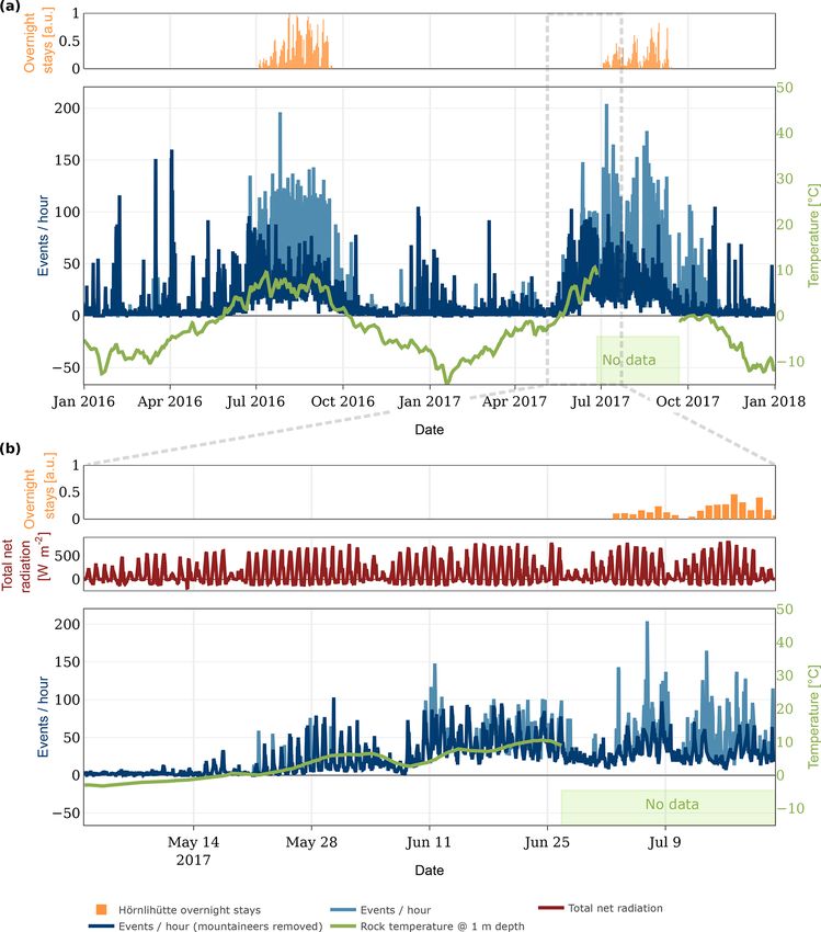
M. Meyer et al.: Systematic identification of external influences in multi-year microseismic recordings                           173

site requiring substantial expert knowledge for a very ardu-
ous, time-consuming task. The aim of this study is to use a
semi-automatic workflow to train a classifier which enables
the automatic identification of unwanted external influences
in real-world microseismic data. By these means, the geo-
physical phenomena of interest can be analyzed without the
distortions of external influences.
    To address these problems, this paper contains the follow-   Figure 1. Real-world measurement signals contain the phenom-
ing contributions. We propose a strategy to identify and deal    ena of interest superimposed with external influences. If directly
with unwanted external influences in multi-sensor, multi-        analyzed, the results are perturbed by the external influences. In
year experiments. We compare the suitability of multiple al-     contrast to this approach (dashed lines), in this paper, we suggest
                                                                 a systematic and automated approach to first identify a multitude
gorithms for mountaineer detection using a combination of
                                                                 of external influence sources in microseismic signals using a classi-
microseismic signals and time-lapse images. We propose a         fier. The classifier result data can then be used to quantify unwanted
convolutional neural network (CNN) for source identifica-        signal components as well as drive more extensive and powerful
tion. We exemplify our strategy for the case of source iden-     event detection and characterization methods leveraging combina-
tification on real-world microseismic data using monitoring      tions of both the signals as well-labeled and classified noise data
data in steep, fractured bedrock permafrost. We further pro-     (solid lines).
vide the real-world microseismic and image data as an an-
notated dataset containing data from a period of 2 years as
well as an open-source implementation of the algorithms pre-     time periods when mountaineers are present and when they
sented.                                                          are not, which we use as a case study in the evaluation section
                                                                 of this paper to exemplify our method.
                                                                     Figure 2 illustrates the overall concept in detail. In a first
2   Concept of the classification method                         step, the available data sources of a case study are assessed
                                                                 and cataloged. Given a case study (Sect. 3) consisting of mul-
In this work, we present a systematic and automated ap-          tiple sensors, one or more sensor signals are specified as pri-
proach to identify unwanted external influences in long-         mary signals (for example, the microseismic signals, high-
term, real-world microseismic datasets and prepare these         lighted with a light green arrow in the figure) targeted by
data for subsequent analysis using a domain-specific anal-       a subsequent domain-specific analysis method. Additionally,
ysis method, as illustrated in Fig. 1. Traditionally, the sig-   secondary data (highlighted with dark blue arrows) are cho-
nal, consisting of the phenomena of interest and superim-        sen to support the classification of external influences con-
posed external influences, is analyzed directly as described     tained in the primary signal. Conceptually, these secondary
earlier. However, this analysis might suffer from distortion     data can be of different nature, either different sensor sig-
through the external influences. By using additional sensors     nals, e.g., time-lapse images or weather data, or auxiliary
like weather stations, cameras or microphones and external       data such as local observations or helicopter flight data. All
knowledge such as helicopter flight plans or mountain hut        data sources are combined into a dataset. However, this re-
(Hörnlihütte) occupancy, it is possible to semi-automatically    sulting dataset is not yet annotated as required to perform
label events originating from non-geophysical sources, such      domain-specific analysis leveraging the identified and quan-
as helicopters, footsteps or wind without the need of expert     tified external influences.
knowledge. Such “external” information sources can be used           Two key challenges need to be addressed in order to es-
to train an algorithm that is then able to identify unwanted     tablish such an annotated dataset by automatic classification:
external influence. Using this approach, multiple external       (i) suitable data types need to be selected for classification
influences are first classified and labeled in an automated      since not every data type can be used to continuously clas-
preprocessing step with the help of state-of-the-art machine     sify every external influence (for example, wind sensors are
learning methods. Subsequent to this classification, the addi-   not designed to capture the sound of footsteps; flight data
tional information can be used for domain-specific analysis,     may not be available for each time step) and (ii) a single
for example, to separate geophysical and unwanted events         (preferred) or at least a set of suitable, well-performing clas-
triggered by a simple event detector such as an STA/LTA          sifiers has to be found for each type of external influence
event detector. Alternatively, more complex approaches can       source. Once these challenges have been solved, a subset of
be used, taking into account signal content, event detections    the dataset is manually annotated in order to select and train
and classifier labels of the external influences. However, the   the classifier(s) in a “preparatory” phase required to be per-
specifics of such advanced domain-specific analysis meth-        formed only once, which includes manual data assessment
ods are beyond the scope of this paper and subject to future     (Sect. 4) as well as classifier selection and training (Sect. 5).
work. A basic example of a custom domain-specific analysis       The trained classifier is then used in an automated setup to
method is the estimation of separate STA/LTA event rates for     annotate the whole dataset (Sect. 6). This “execution” phase

www.earth-surf-dynam.net/7/171/2019/                                                    Earth Surf. Dynam., 7, 171–190, 2019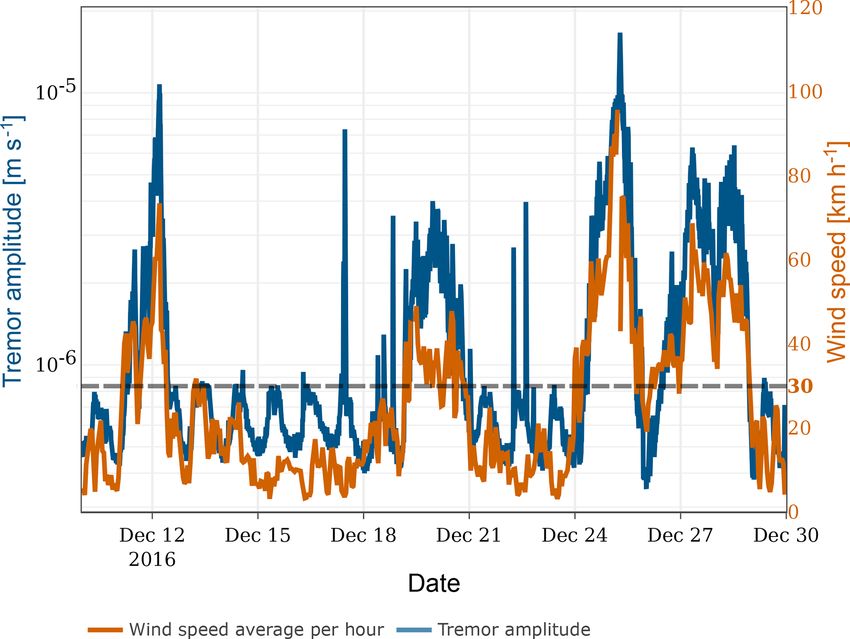
174 M. Meyer et al.: Systematic identification of external influences in multi-year microseismic recordings
Figure 2. Conceptual illustration of the classification method to enable domain-specific analysis of a primary sensor signal (in our case,
microseismic signals denoted by the light green arrow) based on annotated datasets: a subset of the dataset, containing both sensor and
auxiliary data, is used to select and train a classifier that is subsequently applied to the whole dataset. By automatically and systematically
annotating the whole dataset of the primary signal of concern, advanced methods can be applied that are able to leverage both multi-sensor
data as well as annotation information.
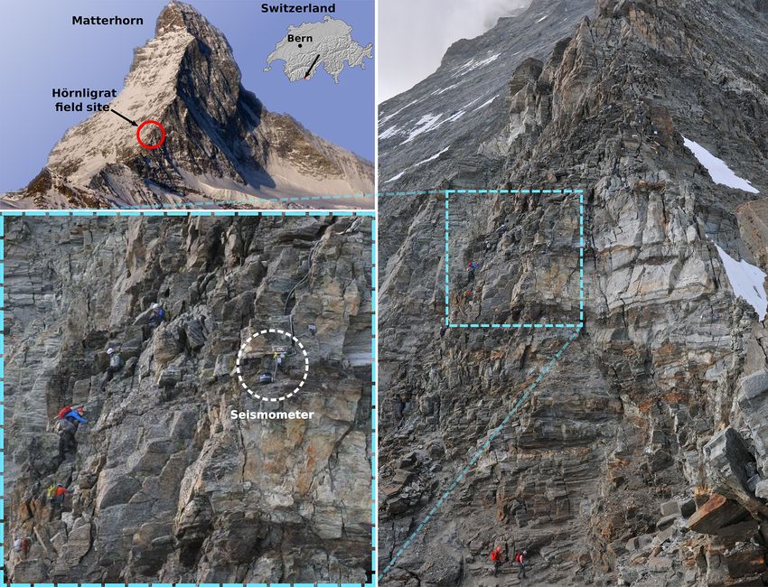
can be performed in a one-shot fashion (post-processing all tion as well as some backdrop areas further away on the
data in one effort) or executed regularly, for example, on a mountain ridge. Figure 3 shows an overview of the field
daily or weekly basis if applied to continuously retrieved site including the location of the seismometer and an ex-
real-time monitoring data. This additional information can be ample image acquired with the camera. The standard image
used to perform a subsequent domain-specific analysis. This size is 1424 × 2144 pixels captured every 4 min. The Vaisala
study concludes with an evaluation (Sect. 7) and discussion WXT520 weather data as well as the rock surface tempera-
(Sect. 8) of the presented method. ture are transmitted using a custom wireless sensor network
infrastructure. A new measurement is performed on the sen-
sors every 2 min and transmitted to the base station, resulting
3 Case study in a sampling rate of 30 samples h−1 .
Significant data gaps are prevented by using solar panels,
The data used in this paper originate from a multi-sensor
durable batteries and field-tested sensors, but given the cir-
and multi-year experiment (Weber et al., 2018b) focus-
cumstances on such a demanding high-alpine field site, cer-
ing on slope stability in high-alpine permafrost rock walls
tain outages of single sensors, for example, due to power
and understanding the underlying processes. Specifically,
failures or during maintenance, could not be prevented. Nev-
the sensor data are collected at the site of the 2003 rock-
ertheless, this dataset constitutes an extensive and close-to-
fall event on the Matterhorn Hörnligrat (Zermatt, Switzer-
complete dataset.
land) at 3500 m a.s.l., where an ensemble of different sen-
The recordings of the case study were affected by external
sors has monitored the rockfall scar and surrounding environ-
influences, especially mountaineers and wind. This reduced
ment over the past 10 years. Relevant for this work are data
the set of possible analysis tools. Auxiliary data which help
from a three-component seismometer (Lennartz LE-3Dlite
to characterize the external influences are collected in addi-
MkIII), images from a remote-controlled high-resolution
tion to the continuous data from the sensors. In the presented
camera (Nikon D300, 24 mm fixed focus), rock surface tem-
case, the auxiliary data are non-continuous and consist of lo-
perature measurements, net radiation measurements and am-
cal observations, preprocessed STA/LTA triggers from We-
bient weather conditions, specifically wind speed from a co-
ber et al. (2018b), accommodation occupancy of a nearby
located local weather station (Vaisala WXT520).
hut and a non-exhaustive list of helicopter flight data from a
The seismometer applied in the case study presented is
duration of approximately 7 weeks provided by a local heli-
used to assess the seismic activity by using an STA/LTA
copter company.
event detector, which means for our application that the seis-
In following, we use this case study to exemplify our
mometer is chosen as the primary sensor and STA/LTA trig-
method, which was presented in the previous sections.
gering is used as the reference method. Seismic data are
recorded locally using a Nanometrics Centaur digitizer and
transferred daily by means of directional Wi-Fi. The data are 4 Manual data assessment
processed on demand using STA/LTA triggering. The high-
resolution camera’s (Keller et al., 2009) field of view cov- A ground truth is often needed for state-of-the-art classifiers
ers the immediate surroundings of the seismic sensor loca- (such as artificial neural networks). To establish this ground
Earth Surf. Dynam., 7, 171–190, 2019 www.earth-surf-dynam.net/7/171/2019/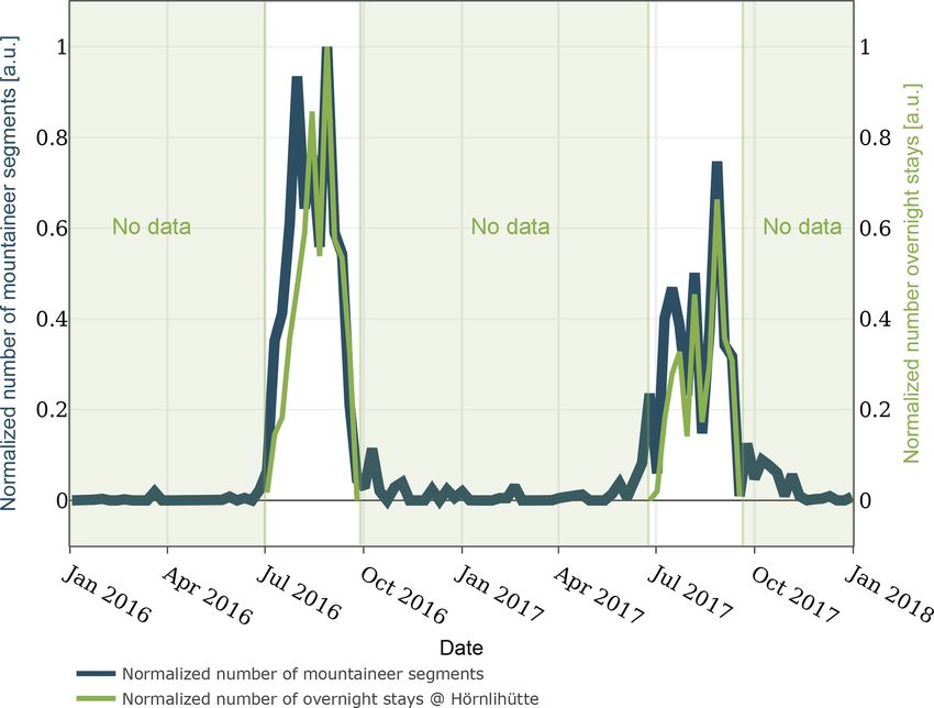
M. Meyer et al.: Systematic identification of external influences in multi-year microseismic recordings                               175

Figure 3. The field site is located on the Matterhorn Hörnligrat at 3500 m a.s.l. which is denoted with a red circle. The photograph on the
right is taken by a remotely controlled DSLR camera at the field site on 4 August 2016, 12:00:11 CET. The seismometer of interest (white
circle) is located on a rock instability which is close to a frequently used climbing route.

truth while reducing the amount of manual labor, only a sub-            ability for classification given the task and the data. A se-
set of the dataset is selected and used in a manual data as-            lection of classifiers is therefore trained and tested with the
sessment phase, which consists of data evaluation, classifier           annotated subset and optimized for best performance, which
training and classifier selection as depicted in Fig. 4. Data           can, for example, be done by selecting the classifier with the
evaluation can be subdivided into four parts: (i) character-            lowest error rate on a defined test set. The classifier selection,
ization of external influences in the primary signal (that is           training and optimization is repeated until a sufficiently good
the relation between primary and secondary signals), (ii) an-           set of classifiers has been found. This suitability is defined
notating the subset based on the primary and secondary sig-             by the user and can, for example, mean that the classifier is
nals, (iii) selecting the data types suitable for classification        better than a critical error rate. These classifiers can then be
and (iv) performing a first statistical evaluation with the an-         used for application in the automatic classification process.
notated dataset, which facilitates the selection of a classifier.          In the following, the previously explained method will be
Characterization and statistical evaluation are the only steps          exemplified for wind and mountaineer detection using micro-
where domain expertise is required while it is not required             seismic, wind and image data from a real-world experiment.
for the time- and labor-intensive annotation process.                   The required steps of subset creation, characterization, anno-
   The classifier selection and training phase presumes the             tation, statistical evaluation and the selection of the data type
availability of a variety of classifiers for different input data       for classification are explained. Before an annotated subset
types, for example, the broad range of available image clas-            can be created the collected, data must be characterized for
sifiers (Russakovsky et al., 2015). The classifiers do not per-         their usefulness in the annotation process, i.e., which data
form equally well on the given task with the given subset.              type can be used to annotate which external influence.
Therefore, classifiers have to be selected based on their suit-

www.earth-surf-dynam.net/7/171/2019/                                                          Earth Surf. Dynam., 7, 171–190, 2019
176                    M. Meyer et al.: Systematic identification of external influences in multi-year microseismic recordings

Figure 4. The manual preparation phase is subdivided into data evaluation (a) and classifier selection and training (b). First, the data
subset is characterized and annotated. This information can be used to do a statistical evaluation and select data types which are useful for
classification. Domain experts are not required for the labor-intensive task of annotation. The classifiers are selected, trained and optimized
in a feedback loop until the best set of classifiers is found.

4.1   Characterization                                                    sources on a larger time frame. Mountaineers, for example,
                                                                          show characteristic patterns of increasing or decreasing loud-
The seismometer captures elastic waves originating from dif-              ness, and helicopters have distinct spectral patterns, which
ferent sources. In this study, we will consider multiple non-             could be beneficial to classify these sources. Additionally, the
geophysical sources, which are mountaineers, helicopters,                 images captured on site show when a mountaineer is present
wind and rockfalls. Time periods where the aforementioned                 (see Fig. 3), but due to fog, lens flares or snow on the lens,
sources cannot be identified are considered as relevant, and              the visibility can be limited. The limited visibility needs to be
thus we will include them in our analysis as a fifth source,              taken into account for when seismic data are to be annotated
the “unknown” source. The mountaineer impact will be char-                with the help of images. Another limiting factor is the tempo-
acterized on a long-term scale by correlating with hut ac-                ral resolution of one image every 4 min since mountaineers
commodation occupancy (see Fig. 10) and on a short-scale                  could have moved through the camera’s field of view in be-
by person identification on images. Helicopter examples are               tween two images.
identified by using flight data and local observations. By ana-              The wind sensor can directly be used to identify the impact
lyzing spectrograms, one can get an intuitive feeling for what            on the seismic sensor. Figure 6 illustrates the correlation be-
mountaineers or helicopters “look” like, which facilitates the            tween tremor amplitude and wind speed. Tremor amplitude
manual annotation process. In Fig. 5, different recordings                is the frequency-selective, median, absolute ground velocity
from the field site are illustrated, which have been picked by            and has been calculated for the frequency range of 1–60 Hz
using the additional information described at the beginning               according to Bartholomaus et al. (2015). By manually an-
of this section. For six different examples, the time domain              alyzing the correlation between tremor amplitude and wind
signal, its corresponding spectrogram and STA/LTA triggers                speed, it can be deduced that wind speeds above approxi-
are depicted. The settings for the detector are the same for all          mately 30 km h−1 have a visible influence on the tremor am-
the subsequent plots. It becomes apparent in Fig. 5b–c that               plitude.
anthropogenic noise, such as mountaineers walking by or he-                  Rockfalls can best be identified by local observations since
licopters, is recorded by seismometers. Moreover, it becomes              the camera captures only a small fraction of the receptive
apparent that it might be feasible to assess non-geophysical              range of the seismometers. Figure 5e illustrates the seis-

Earth Surf. Dynam., 7, 171–190, 2019                                                            www.earth-surf-dynam.net/7/171/2019/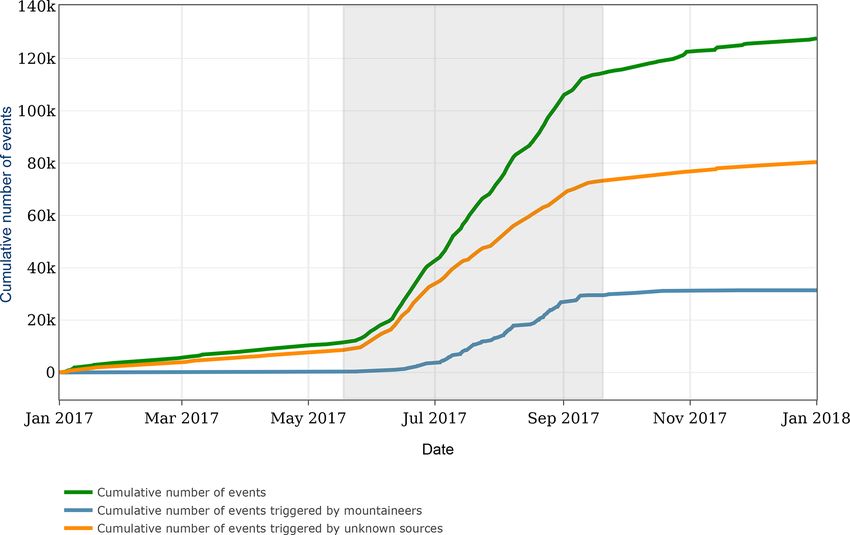
M. Meyer et al.: Systematic identification of external influences in multi-year microseismic recordings                                    177

Figure 5. Microseismic signals and the impact of external influences. (a) During a period of little anthropogenic noise, the seismic activity is
dominant. (b) In the spectrogram, the influence of mountaineers becomes apparent. Shown are seismic signatures of (c) a helicopter in close
spatial proximity to the seismometer, (d) wind influences on the signal and (e) a rockfall in close proximity to the seismometer. The red dots
in the signal plots indicate the timestamps of the STA/LTA triggers from Weber et al. (2018b).

mic signature of a rockfall. The number of rockfall observa-              the geophysical application (Colombero et al., 2018; Weber
tions and rockfalls caught on camera is however very limited.             et al., 2018b).
Therefore, it is most likely that we were unable to annotate
all rockfall occurrences. As a consequence, we will not con-              4.2    Annotation
sider a rockfall classifier in this study.
   It can be seen in Fig. 5a that during a period which is not            The continuous microseismic signals are segmented for an-
strongly influenced by external influences the spectrogram                notation and evaluation. Figure 7 provides an overview of
shows mainly energy in the lower frequencies with occa-                   the three segmentation types, event-linked segments, image-
sional broadband impulses.                                                linked segments and consecutive segments. Image-linked
   The red circles in the subplots in Fig. 5 indicate the times-          segments are extracted due to the fact that a meaningful re-
tamps of the STA/LTA events for a specific geophysical anal-              lation between seismic information and photos is only given
ysis (Weber et al., 2018b). By varying the threshold of the               in close temporal proximity. Therefore, images and micro-
STA/LTA event trigger, the number of events triggered by                  seismic data are linked in the following way. For each image,
mountaineers can be reduced. However, since the STA/LTA                   a 2 min microseismic segment is extracted from the contin-
event detector cannot discriminate between events from geo-               uous microseismic signal. The microseismic segment’s start
physical sources and events from mountaineers, changing the               time is set to 1 min before the image timestamp. Event-linked
threshold would also influence the detection of events from               segments are extracted based on the STA/LTA triggers from
geophysical sources. This fact would affect the quality of                Weber et al. (2018b). For each trigger, the 10 s following
the analysis since the STA/LTA settings are determined by                 the timestamp of the trigger are extracted from the micro-
                                                                          seismic signal. Consecutive segments are 2 min segments se-

www.earth-surf-dynam.net/7/171/2019/                                                              Earth Surf. Dynam., 7, 171–190, 2019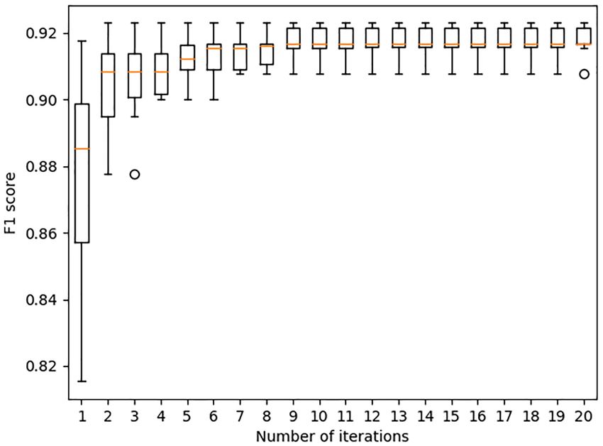
178 M. Meyer et al.: Systematic identification of external influences in multi-year microseismic recordings
For mountaineer classification, the required label is
“mountaineer” but additional labels will be annotated which
could be beneficial for classifier training and statistical analy-
sis. These labels are “helicopters”, “rockfalls”, “wind”, “low
visibility” (if the lens is partially obscured) and “lens flares”.
The “wind” label applies to segments where the wind speed
is higher than 30 km h−1 , which is the lower bound for no-
ticeable wind impact as resulted from Sect. 4.1.
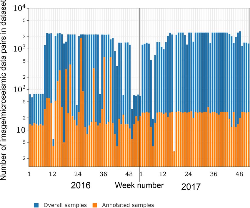
Figure 8 depicts the availability of image-linked segments
per week during the relevant time frame. A fraction of the
data is manually labeled by the authors, which is illustrated
in Fig. 8. Two sets are created: a training set containing 5579
samples from the year 2016, and a test set containing 1260
data samples from 2017. The test set has been sampled ran-
domly to avoid any human prejudgment. For each day in
2017, four samples have been chosen randomly, which are
Figure 6. Impact of wind (light orange) on the seismic signal. The then labeled and added to the test set. The training set has
tremor amplitude (dark blue) is calculated according to Bartholo- been specifically sampled to include enough training data for
maus et al. (2015). The effect of wind speed on tremor amplitude each category. This means, for example, that more moun-
becomes apparent for wind speeds above approximately 30 km h−1 . taineer samples come from the summer period where the
Note the different scales on the y axes. climbing route is most frequently used. The number of ver-
ified rockfalls and helicopters is non-representative, and al-
though helicopters can be manually identified from spectro-
grams, the significance of these annotations is not given due
to the limited ground truth from the secondary source. There-
fore, for the rest of this study, we will focus on mountaineers
for qualitative evaluation. For statistical evaluation, we will
however use the manually annotated helicopter and rockfall
samples to exclude them from the analysis. The labels for all
categories slightly differ for microseismic data and images
since the types of sources which can be registered by each
sensor differ. This means, for instance, that not every classi-
Figure 7. Illustration of microseismic segmentation. Event-linked fier uses all labels for training (for example, a microseismic
segments are 10 s segments starting on event timestamps. Image- classifier cannot detect a lens flare). It also means that for the
linked segments are 2 min segments centered around an image same time instance one label might apply to the image but
timestamp. Consecutive segments are 2 min segments sequentially not to the image-linked microseismic segment (for example,
extracted from the continuous microseismic signal.
mountaineers are audible but the image is partially obscured
and the mountaineer is not visible). This becomes relevant in
Sect. 5.3.4 when multiple classifiers are used for ensemble
quentially extracted from the continuous microseismic sig-
classification.
nal.
Only the image-linked segments are used during annota-
tion; their label can, however, be transferred to other seg- 4.3 Data type selection
mentation types by assigning the image-linked label to over-
After the influences have been characterized, the data type
lapping event-linked or consecutive segments. Image-linked
which best describe each influence needs to be selected. The
and event-linked segments are used during data evaluation
wind sensor delivers a continuous data stream and a direct
and classifier training. Consecutive segments are used for au-
measure of the external influence. In contrast, mountaineers,
tomatic classification on the complete dataset. Here, falsely
helicopters and rockfalls cannot directly be identified. A data
classified segments are reduced by assigning each segment a
type including information about these external influences
validity range. A segment classified as mountaineer is only
needs to be selected. Local observations, accommodation oc-
considered correct if the distance to the next (or previous)
cupancy and flight data can be discarded for the use as clas-
mountaineer is less than 5 min. This is based on an estima-
sifier input since the data cannot be continuously collected.
tion of how long the mountaineers are typically in the audible
According to Sect. 4.1, it seems possible to identify moun-
range of the seismometer.
taineers, helicopters and rockfalls from microseismic data.
Moreover, mountaineers can also be identified from images.
Earth Surf. Dynam., 7, 171–190, 2019 www.earth-surf-dynam.net/7/171/2019/M. Meyer et al.: Systematic identification of external influences in multi-year microseismic recordings 179
where ∗ denotes the convolution operator, g(·) is a nonlinear
function, Ij is an input channel, bk is the bias related to the
feature map FH,k , and wk,j is the kernel related to the input
image Ij and feature map FH,k . Kernel and bias are trainable
parameters of each layer. This principle can be applied to
subsequent convolutional layers. Additionally, a strided con-
volution can be used which effectively reduces the dimen-
sion of a feature map as illustrated by L1 in Fig. 9. In an
all-convolutional neural network (Springenberg et al., 2014),
the feature maps of the output convolutional layer are aver-
aged per channel. In our case, the number of output channels
is chosen to be the number of event sources to be detected.
Subsequent scaling and a final (nonlinear) activation func-
tion are applied. If trained correctly, each output represents
the probability that the input contains the respective event
source. In our case, this training is performed by calculat-
ing the binary cross-entropy between the network output and
the ground truth. The error is back-propagated through the
Figure 8. Number of image/microseismic data pairs in the dataset neural network and the parameters are updated. The training
(dark blue) and in the annotated subset (light orange) displayed over procedure is performed for all samples in the dataset and is
the week number of the years 2016 and 2017. Note the logarithmic
repeated for multiple epochs.
scale on the y axis.
5.2 Classifier selection
As a consequence, the data types selected to perform clas-
Multiple classifiers are available for the previously selected
sification are microseismic data, images and wind data. The
data types: wind data, images and microseismic data.
microseismic data used are the signals from the three com-
For wind data, a simple threshold classifier can be used,
ponents of the seismometer.
which indicates wind influences based on the wind speed.
For simplicity, the classifier labels time periods with wind
5 Classifier selection and training speed above 30 km h−1 as “wind”. For images, a convolu-
tional neural network is selected to classify the presence of
The following section describes the classifier preselection, mountaineers in the image. The image classifier architecture
training, testing and how the classifiers are used to annotate is selected from the large pool of available image classifiers
the whole data stream as illustrated in Fig. 4b. First, a brief (Russakovsky et al., 2015). For microseismic data, three dif-
introduction to convolutional neural networks is given. If the ferent classifiers will be preselected: (i) a footstep detector
reader is unfamiliar with neural networks, we recommend to based on manually selected features (standard deviation, kur-
read additional literature (Goodfellow et al., 2016). tosis and frequency band energies) using a linear support
vector machine (LSVM) similar to the detector used in An-
chal et al. (2018), (ii) a seismic event classifier adopted from
5.1 Convolutional neural networks Perol et al. (2018) and (iii) a non-geophysical event classi-
fier which we call MicroseismicCNN. We re-implemented
Convolutional neural networks have gained a lot of interest
the first two algorithms based on the information from the
due to their advanced feature extraction and classification
respective papers. The third is a major contribution in this
capabilities. A convolutional neural network contains mul-
paper and has been specifically designed to identify non-
tiple adoptable parameters which can be updated in an iter-
geophysical sources in microseismic data.
ative optimization procedure. This fact makes them generi-
The proposed convolutional neural network (CNN) to
cally applicable to a large range of datasets and a large range
identify non-geophysical sources in microseismic signals
of different tasks. The convolutional neural network consists
uses a time–frequency signal representation as input and con-
of multiple so-called convolutional layers. A convolutional
sists of 2-D convolutional layers. Each component of the time
layer transforms its input signal with ci channels into ch fea-
domain signal, sampled at 1 kHz, is first offset compensated
ture maps as illustrated in Fig. 9. A hidden feature map FH,k
and then transformed with a short-time Fourier transforma-
is calculated according to
tion (STFT). Subsequently, the STFT output is further pro-
ci
! cessed by selecting the frequency range from 2 to 250 Hz
X
FH,k = g Ij∗ wk,j + bk , and subdividing it into 64 linearly spaced bands. This time–
j =1 frequency representation of the three seismometer compo-
www.earth-surf-dynam.net/7/171/2019/ Earth Surf. Dynam., 7, 171–190, 2019180 M. Meyer et al.: Systematic identification of external influences in multi-year microseismic recordings
Figure 9. Simplified illustration of a convolutional neural network. An input signal, for example, an image or spectrogram, with a given
number of channels ci is processed by a convolutional layer LH . The output of the layer is a feature map with ch channels. Layer LO takes
the hidden feature map as input and performs a strided convolution which results in the output feature map with reduced dimensions and
number of channels co . Global average pooling is performed per channel and additional scaling and a final activation are applied.
nents can be interpreted as 2-D signal with three channels, Table 1. Layout of the proposed non-geophysical event classifier,
which is the network input. The network consists of multiple consisting of multiple layers which are executed in sequential order.
convolutional, batch normalization and dropout layers, as de- The convolutional neural network consists of multiple 2-D convolu-
picted in Table 1. Except for the first convolutional layer, all tional layers (Conv2D) with batch normalization (BatchNorm) and
convolutional layers are followed by batch normalization and rectified linear unit (ReLU) activation. Dropout layers are used to
minimize overfitting. The sequence of global average pooling layer,
rectified linear unit (ReLU) activation. Finally, a set of global
a scaling layer and the sigmoid activation compute one value be-
average pooling layer, dropout, trainable scaling (in the form tween 0 and 1 resembling the probability of a detected mountaineer.
of a convolutional layer with kernel size 1) and sigmoid ac-
tivation reduces the features to one value representing the Output
probability that a mountaineer is in the microseismic signal. Layer Stride
channels
In total, the network has 30 243 parameters. In this architec-
ture, multiple measures have been taken to minimize over- Conv2D + BatchNorm + Linear 1 32
fitting: the network is all-convolutional (Springenberg et al., Conv2D + BatchNorm + ReLU 2 32
Dropout – 32
2014), batch normalization (Ioffe and Szegedy, 2015) and
Conv2D + BatchNorm + ReLU 2 32
dropout (Srivastava et al., 2014) are used and the size of the Dropout – 32
network is small compared to recent audio classification net- Conv2D + BatchNorm + ReLU 1 32
works (Hershey et al., 2016). Conv2D + ReLU 1 32
Dropout – 32
Conv2D + ReLU 1 1
5.3 Training and testing Global average pooling 1 1
Dropout – 1
We will evaluate the microseismic algorithms in two scenar- Conv2D 1 1
ios in Sect. 7.1. In this section, we describe the training and Sigmoid activation – 1
test setup for the two scenarios as well as for image and en-
semble classification. In the first scenario, event-linked seg-
ments are classified. In the second scenario, the classifiers on of the validation set is calculated, and based on it, the best
image-linked segments are compared. The second scenario performing network version is selected. The F1 score is de-
stems from the fact that the characterization from Sect. 4.1 fined as
suggested that using a longer temporal input window could 2 · true positive
lead to a better classification because it can capture more F1 score = .
2 · true positive + false negative + false positive
characteristics of a mountaineer. Training is performed with
the annotated subset from Sect. 4, and a random 10 % of the The threshold for the network’s output is determined by run-
training set are used as the validation set, which is never used ning a parameter search with the validation set’s F1 score as
during training. For the non-geophysical and seismic event the metric. Training was performed in batches of 32 sam-
classifiers, the number of epochs has been fixed to 100 and ples with the ADAM (Kingma and Ba, 2014) optimizer and
for the image classifier to 20. After each epoch, the F1 score cross-entropy loss. The Keras (Chollet, 2015) framework
Earth Surf. Dynam., 7, 171–190, 2019 www.earth-surf-dynam.net/7/171/2019/M. Meyer et al.: Systematic identification of external influences in multi-year microseismic recordings 181
with a TensorFlow backend (Abadi et al., 2015) was used metrics can be calculated with the following assumption: if
to implement and train the network. The authors of the seis- any of the event-linked segments which are overlapping with
mic event classifier (Perol et al., 2018) provide TensorFlow an image-linked segment are classified as mountaineer, the
source code, but to keep the training procedure the same, it image-linked segment is considered to be classified as moun-
was re-implemented with the Keras framework. The footstep taineer as well.
detector is trained with scikit-learn (Pedregosa et al., 2011). The results will be discussed in Sect. 7.1.
Testing is performed on the test set which is independent of
the training set and has not been used during training. The 5.3.3 Image classification
metric error rate and F1 score are calculated.
It is common to do multiple iterations of training and test- Since convolutional neural networks are a predominant tech-
ing to get the best-performing classifier instance. We per- nique for image classification, a variety of network archi-
form a preliminary parameter search to estimate the number tectures have been developed. For this study, the MobileNet
of iterations. The estimation takes into account the number (Howard et al., 2017) architecture is used. The number of
of training types (10 different classifiers need to be trained) labeled images is small in comparison to the network size
given the limited processing capabilities. As a result of the (approximately 3.2 million parameters) and training the net-
search, we train and test 10 iterations and select the best clas- work on the Matterhorn images will lead to overfitting on the
sifier instance of each classifier type to evaluate and compare small dataset. To reduce overfitting, a MobileNet implemen-
their performance in Sect. 7. tation which has been pre-trained on ImageNet (Deng et al.,
The input of the microseismic classifiers must be variable 2009), a large-scale image dataset, will be used. Retraining
to be able to perform classification on event-linked segments is required since ImageNet has a different application fo-
and image-linked segments. Due to the principle of convolu- cus than this study. The climbing route, containing the sub-
tional layers, the CNN architectures are independent of the ject of interest, only covers a tiny fraction of the image, and
input size, and therefore no architectural changes have to be rescaling the image to 224 × 224 pixels, the input size of the
performed. The footstep detector’s input features are aver- MobileNet, would lead to vanishing mountaineers (compare
aged over time by design and are thus also time invariant. Fig. 3). However, the image size cannot be chosen arbitrarily
large since a larger input requires more memory and results
5.3.1 Event-linked segments experiment
in a larger runtime. To overcome this problem, the image has
been scaled to 448 × 672 pixels, and although the input size
Literature suggests that STA/LTA cannot distinguish geo- differs from the pre-trained version, network retraining still
physical sources from non-geophysical sources (Allen, benefits from pre-trained weights. Data augmentation is used
1978). Therefore, the first microseismic experiment investi- to minimize overfitting. For data augmentation, each image
gates if the presented algorithms can distinguish events in- is slightly zoomed in and shifted in width and height. The
duced by mountaineers from other events in the signal. The network has been trained to detect five different categories.
event-linked segments are used for training and evaluation. In this paper, only the metrics for mountaineers are of inter-
The results will be discussed in Sect. 7.1. est for the evaluation and the metrics for the other labels are
discarded in the following. However, all categories are rel-
5.3.2 Image-linked segments experiment
evant for a successful training of the mountaineer classifier.
These categories consist of “mountaineer”, “low visibility”
In the second microseismic experiment, the image-linked (if the lens is partially obscured), “lens flare”, “snowy” (if
segments will be used. Each classifier is trained and evalu- the seismometer is covered in snow) and “bad weather” (as
ated on the image-linked segments. The training parameters far as it can be deduced from the image).
for training the classifiers on image-linked segments are as
before but additionally data augmentation is used to mini- 5.3.4 Ensemble
mize overfitting. Data augmentation includes random circu-
lar shift and random cropping on the time axis. Moreover, to In certain cases, a sensor cannot identify a mountaineer al-
account for the uneven distribution in the dataset, it is made though there is one; for example, the seismometers cannot
sure that during training the convolutional neural networks detect when the mountaineer is not moving or the camera
see one example of a mountaineer every batch. The learning does not capture the mountaineer if the visibility is low.
rate is set to 0.0001, which was determined with a prelimi- The usage of multiple classifiers can be beneficial in these
nary parameter search. The classifiers are then evaluated on cases. In our case, microseismic and image classifiers will be
the image-linked segments. jointly used for mountaineer prediction. Since microseismic
To be able to compare the results of the classifiers trained labels and image labels are slightly different, as discussed in
on image-linked segments to the classifiers trained on event- Sect. 4.2, the ground truth labels must be combined. For a
linked segments (Sect. 5.3.1), the classifiers from Sect. 5.3.1 given category, a sample is labeled true if any of microseis-
will be evaluated on the image-linked segments as well. The mic or image labels are true (logical disjunction). After indi-
www.earth-surf-dynam.net/7/171/2019/ Earth Surf. Dynam., 7, 171–190, 2019182 M. Meyer et al.: Systematic identification of external influences in multi-year microseismic recordings
vidual prediction by each classifier, the outputs of the clas- Table 2. Results of the different classifiers. The addition of
sifiers are combined similarly and can be compared to the “(events)” labels the classifier versions trained on event-linked seg-
ground truth. ments
Error rate F1 score
5.4 Optimization
Event-linked segments
Due to potential human errors during data labeling, the train-
ing set has to be regarded as a weakly labeled dataset. Such Footstep detector (events) 0.1702 0.7692
Seismic event classifier (events) 0.1250 0.8291
datasets can lead to a worse classifier performance. To over-
MicroseismicCNN (events) 0.0641 0.9062
come this issue, a human-in-the-loop approach is followed,
where a preliminary set of classifiers is trained on the training Image-linked segments
set. In the next step, each sample of the dataset is automat- Footstep detector (events) 0.0706 0.5389
ically classified. This procedure produces a number of true Seismic event classifier (events) 0.0540 0.6047
positives, false positives and true negatives. These samples MicroseismicCNN (events) 0.0309 0.731
are then manually relabeled and the labels for the dataset are Footstep detector 0.0952 0.52
updated based on human review. The procedure is repeated Seismic event classifier 0.0313 0.7383
multiple times. However, this does not completely avoid the MicroseismicCNN 0.0096 0.9167
possibility of falsely labeled samples in the dataset, since the Image classifier 0.0088 0.9134
algorithm might not find all human-labeled false negatives, Ensemble 0.0079 0.9383
but it increases the accuracy significantly. The impact of false
labels on classifier performance will be evaluated in Sect. 7.1.
6 Automatic classification
0.0952 on image-linked segments. Both convolutional neural
In Sect. 7.1, it will be shown that the best set of classifiers networks score a lower error rate on image-linked segments
is the ensemble of image classifier and MicroseismicCNN. of 0.0096 (MicroseismicCNN) and 0.0313 (seismic event
Therefore, the trained image classifiers and Microseismic- classifier). For the given dataset, our proposed Microseis-
CNN classifier are used to annotate the whole time period micCNN network outperforms the seismic event classifier
of collected data to quantitatively assess the impact of moun- in both the event-linked segment experiment as well as the
taineers. The image classifier and the MicroseismicCNN will image-linked segment experiment. The MicroseismicCNN
be used to classify all the images and microseismic data, re- using a longer input window (trained on image-linked seg-
spectively. The consecutive segments and images are used ments) is comparable to classification on images and outper-
for prediction. To avoid false positives, we assume that a forms the classifier trained on event-linked segments. When
mountaineer requires a certain amount of time to pass by the combining image and microseismic classifiers, the best re-
seismometer as illustrated in Fig. 7; therefore, a mountaineer sults can be achieved.
annotation is only considered valid if its minimum distance The number of training/test iterations that were run for
to the next (or previous) mountaineer annotation is less than each classifier has been set to 10 through a preliminary pa-
5 min. Subsequently, events within time periods classified as rameter estimation. To validate our choice, we have evalu-
mountaineers are removed and the event count per hour is ated the influences of the number of experiments for only
calculated. one classifier. The performance of the classifier is expected
to depend on the number of training/test iterations (more iter-
7 Evaluation ations indicate a better chance of selecting the best classifier).
However, the computing time is increasing linearly with in-
In the following, the results of the different classifier exper- creasing number of iterations. Hence, a reasonable trade-off
iments described in Sect. 5.3 will be presented to determine between the performance of the classifier and the comput-
the best set of classifiers. Furthermore, in Sect. 7.2 and 7.3, ing time is desired to identify the ideal number of iterations.
results of the automatic annotation process (Sect. 6) will used Figure 11 represents the statistical distribution of the clas-
to evaluate the impact of external influences on the whole sifier’s performance for the different number of training/test
dataset. iterations. Each box plot is based on 10 independent sets of
training/test iterations. While the box indicates the interquar-
tile range (IQR) with the median value in orange, the whisker
7.1 Classifier evaluation
on the appropriate side is taken to 1.5 × IQR from the quar-
The results of the classifier experiments (Table 2) show that tile instead of the maximum or minimum if either type of
the footstep detector is the worst at classifying mountaineers, outlier is present. Beyond the whiskers, data are considered
with an error rate of 0.1702 on event-linked segments and outliers and are plotted as individual points. As can be seen
Earth Surf. Dynam., 7, 171–190, 2019 www.earth-surf-dynam.net/7/171/2019/M. Meyer et al.: Systematic identification of external influences in multi-year microseismic recordings 183 Figure 10. Event count, hut occupancy and rock temperature over time: (a) for the years 2016 and 2017 and (b) for a selected period during defreezing of the rock. The event rate from Weber et al. (2018b) is illustrated in light blue and the rate after removal of mountaineer-induced events in dark blue. The strong variations in event rates correlate with the presence of mountaineers and hut occupancy and in panel (b) with the total net radiation. The impact of mountaineers is significant after 9 July and event detection analysis becomes unreliable. in Fig. 11, the F1 score saturates at nine iterations. Therefore, ence on the classification performance since the mean per- our choice of 10 iterations is a reasonable choice. formance is worse for a high percentage of false labels. In Sect. 5.4, the possibility of falsely labeled training sam- ples has been discussed. As expected, our evaluation in Ta- ble 3 indicates that falsely labeled samples have an influ- www.earth-surf-dynam.net/7/171/2019/ Earth Surf. Dynam., 7, 171–190, 2019
184                     M. Meyer et al.: Systematic identification of external influences in multi-year microseismic recordings

                                                                          can be deduced that the average number of triggered events
                                                                          per hour for times when the signal is influenced by moun-
                                                                          taineers increases by approximately 9 times in comparison to
                                                                          periods without annotated external influences. The effect of
                                                                          wind influences on event rate is not as clear as the influence
                                                                          of mountaineers. The values in Table 4 indicate a decrease
                                                                          of events per hour during wind periods, which will be briefly
                                                                          discussed in Sect. 8.2.
                                                                             As can be seen in Fig. 12, events are triggered over the
                                                                          course of the whole year, whereas events that are annotated as
                                                                          coming from mountaineers occur mainly during the summer
                                                                          period. The main increase in event count occurs during the
                                                                          period when the rock is unfrozen, which unfortunately coin-
                                                                          cides with the period of mountaineer activity. Therefore, it
                                                                          is important to account for the mountaineers. However, even
                                                                          if the mountaineers are not considered, the event count in-
Figure 11. The statistical distribution of the classifier’s perfor-       creases significantly during the unfrozen period. The inter-
mance for the different number of training/test iterations is illus-      pretation of these results will not be part of this study but
trated. Each box plot is based on 10 independent sets of training/test    they are an interesting topic for further research.
iterations. The F1 score saturates after 9 iterations and validates our
choice of 10 iterations.
                                                                          7.3   Automatic annotation in a real-world scenario
Table 3. Influence of falsely labeled data points on the test perfor-     The result of applying the ensemble classifier to the whole
mance. Shown are the mean values over 10 training/test iterations.        dataset is visualized for two time periods in Fig. 10. The
                                                                          figure depicts the event count per hour before and after re-
  False labels (%)        25      12.5      6.25    3.125         0       moving periods of mountaineer activity, as well as the rock
  F1 score (mean)     0.7953    0.8633   0.8761    0.8835    0.8911       temperature, the overnight stays at the Hörnlihütte and the
  Error rate (mean)   0.0208    0.0149   0.0139    0.0129    0.0122       total net radiation. From Fig. 10a, it becomes apparent that
                                                                          the mountaineer activity is mainly present during summer
                                                                          and autumn. An increase is also visible during increasing hut
7.2   Statistical evaluation                                              overnight stays. During winter and spring, only few moun-
                                                                          taineers are detected but some activity peaks remain. By
The annotated test set from Sect. 4.2 and the automatically               manual review, we were able to discard mountaineers as
annotated set from Sect. 6 are used for a statistical evaluation          cause for most of these peaks; however, further investigation
involving the impact of external influences on microseismic               is needed to explain their occurrence.
events. Only data from 2017 are chosen, since wind data are                  Figure 10b focuses on the defreezing period. The zero
not available for the whole training set due to a malfunction             crossing of the rock temperature has a significant impact on
of the weather station in 2016. The experiment from Weber                 the event count variability. A daily pattern becomes visible
et al. (2018b) provides STA/LTA event triggers for 2017. Ta-              starting around the zero crossing. Since few mountaineers are
ble 4 shows statistics for several categories, which are three            detected in May, these can be discarded as the main influence
external influences and one category where none of the three              for these patterns. The total net radiation, however, indicates
external influences are annotated (declared as “unknown”).                an influence of solar radiation on the event count. Further in-
For each category, the total duration of all annotated seg-               depth analysis is needed but this example shows the benefits
ments is given and how many events per hour are triggered. It             of a domain-specific analysis, since the additional informa-
becomes apparent that mountaineers have the biggest impact                tion gives an intuitive description of relevant processes and
on the event analysis. Up to 105.9 events per hour are de-                their interdependencies. After 9 July, the impact of moun-
tected on average during time periods with mountaineer ac-                taineers is significant and the event detection analysis be-
tivity, while during all other time periods the average ranges            comes unreliable. Different evaluation methods are required
from 9.09 to 13.12 events per hour. This finding supports our             to mitigate the influence of mountaineers during these peri-
choice to mainly focus on mountaineers in this paper and                  ods.
shows that mountaineers have a strong impact on the analy-                   Figure 13 depicts that mountaineer predictions and hut oc-
sis. As a consequence, a high activity detected by the event              cupancy correlate well, which indicates that the classifiers
trigger does not correspond to a high seismic activity; thus,             work well. The discrepancy in the first period of each sum-
relying only on this kind of event detection may lead to a                mer needs further investigation. With the annotations for the
false interpretation. From the automatic section in Table 4, it           whole time span, it can be estimated that from all events de-

Earth Surf. Dynam., 7, 171–190, 2019                                                          www.earth-surf-dynam.net/7/171/2019/
You can also read