Machine-learning Approaches to Exoplanet Transit Detection and Candidate Validation in Wide-field Ground-based Surveys
←
→
Page content transcription
If your browser does not render page correctly, please read the page content below

MNRAS 000, 1–15 (2018)                       Preprint 20 November 2018                 Compiled using MNRAS LATEX style file v3.0

                                               Machine-learning Approaches to Exoplanet Transit
                                               Detection and Candidate Validation in Wide-field
                                               Ground-based Surveys

                                                N. Schanche,1 ? A. Collier Cameron,1 G. Hébrard,2 L. Nielsen,3
                                               A. H.M.J. Triaud,4 J.M. Almenara, 5 K.A. Alsubai, 6 D.R. Anderson,7
                                               D.J. Armstrong,8,9 S.C.C. Barros,10 F. Bouchy,3 P. Boumis,11 D.J.A. Brown,8,9
arXiv:1811.07754v1 [astro-ph.EP] 19 Nov 2018

                                               F. Faedi,9,12 K. Hay,1 L. Hebb,13 F. Kiefer,2 L. Mancini,14,15,16,17 P.F.L. Maxted,7
                                               E. Palle,18,19 D.L. Pollacco,8,9 D. Queloz,3,20 B. Smalley,7 S. Udry,12 R. West,8,9
                                               P.J. Wheatley8,9
                                               1 Centre  for Exoplanet Science, SUPA, School of Physics and Astronomy, University of St Andrews, St Andrews KY16 9SS, UK
                                               2 Institut d’astrophysique de Paris, UMR7095 CNRS, Université Pierre & Marie Curie, 98bis boulevard Arago, 75014 Paris, France
                                               3 Observatoire de GenÃĺve, UniversitÃl’ de GenÃĺve, 51 Chemin des Maillettes, CH-1290 Sauverny, Switzerland
                                               4 School of Physics & Astronomy, University of Birmingham, Edgbaston, Birmingham B15 2TT, UK
                                               5 Université Grenoble Alpes, CNRS, IPAG, 38000 Grenoble, France
                                               6 Qatar Environment and Energy Research Institute (QEERI), Hamad Bin Khalifa University (HBKU), Qatar Foundation, Doha, Qatar
                                               7 Astrophysics Group, Keele University, Staffordshire, ST5 5BG, UK
                                               8 Centre for Exoplanets and Habitability, University of Warwick, Gibbet Hill Road, Coventry, CV4 7AL, UK
                                               9 Department of Physics, University of Warwick, Coventry CV4 7AL, UK
                                               10 Instituto de Astrofı́sica e Ciências do Espaço, Universidade do Porto, CAUP, Rua das Estrelas, 4150-762 Porto, Portugal
                                               11 Institute for Astronomy, Astrophysics, Space Applications and Remote Sensing, National Observatory of Athens, 15236 Penteli, Greece
                                               12 INAF - Osservatorio Astrofisico di Catania, Via S. Sofia 78, I-95123 Catania, Italy
                                               13 Hobart and William Smith Colleges, Department of Physics, Geneva, NY 14456, USA
                                               14 Department of Physics, University of Rome Tor Vergata, Via della Ricerca Scientifica 1, 00133 Roma, Italy
                                               15 Max Planck Institue for Astronomy, Königstuhl 17, 69117 Heidelberg, Germany
                                               16 INAF - Astrophysical Observatory of Turin, Via Osservatorio 20, 10025 Pino Torinese, Italy
                                               17 International Institute for Advanced Scientific Studies (IIASS),Via G. Pellegrino 19, I-84019 – Vietri sul Mare (SA), Italy
                                               18 Instituto de Astrosfı́sica de Canarias (IAC), 38205 La Laguna, Tenerife, Spain
                                               19 Departamento de Astrofı́sica, Universidad de La Laguna (ULL), 38206 La Laguna, Tenerife, Spain
                                               20 Cavendish Laboratory, JJ Thompson Avenue, CB3 0HE, Cambridge, UK

                                               Accepted 2018 November 13. Received 2018 October 22; in original form 2018 August 15

                                                                                ABSTRACT

                                                                                     Since the start of the Wide Angle Search for Planets (WASP) program, more
                                                                                than 160 transiting exoplanets have been discovered in the WASP data. In the past,
                                                                                possible transit-like events identified by the WASP pipeline have been vetted by human
                                                                                inspection to eliminate false alarms and obvious false positives. The goal of the present
                                                                                paper is to assess the effectiveness of machine learning as a fast, automated, and
                                                                                reliable means of performing the same functions on ground-based wide-field transit-
                                                                                survey data without human intervention. To this end, we have created training and
                                                                                test datasets made up of stellar light curves showing a variety of signal types including
                                                                                planetary transits, eclipsing binaries, variable stars, and non-periodic signals. We use a
                                                                                combination of machine learning methods including Random Forest Classifiers (RFCs)
                                                                                and Convolutional Neural Networks (CNNs) to distinguish between the different types
                                                                                of signals. The final algorithms correctly identify planets in the test data ∼90% of the
                                                                                time, although each method on its own has a significant fraction of false positives. We
                                                                                find that in practice, a combination of different methods offers the best approach to
                                                                                identifying the most promising exoplanet transit candidates in data from WASP, and
                                                                                by extension similar transit surveys.
                                                                                Key words: planets and satellites: detection - methods: statistical - methods: data
                                                                                analysis
                                               c 2018 The Authors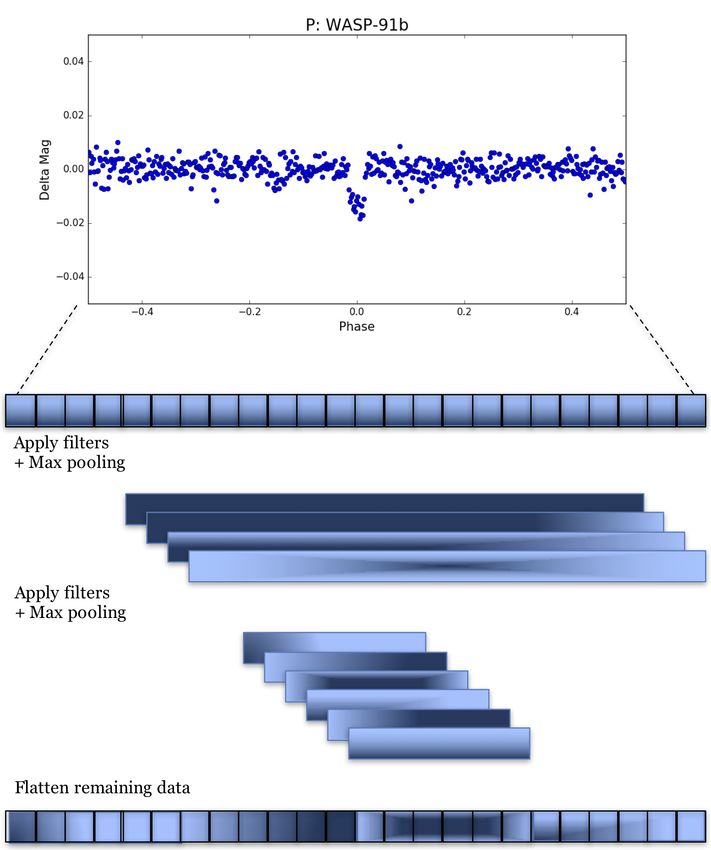
2      N. Schanche et al
1    INTRODUCTION                                                       While Kepler provides an excellent data source for ma-
                                                                   chine learning (regular observations, no atmospheric scatter,
Exoplanet transit surveys such as the Convection Rota-
                                                                   excellent precision, large sample size), similar techniques can
tion and Planetary Transits (CoRoT; Auvergne et al. 2009),
                                                                   also be applied to ground-based surveys, and in fact machine
Hungarian-made Automated Telescope Network (HATnet;
                                                                   learning techniques have recently been incorporated by the
Hartman et al. 2004), HATSouth (Bakos et al. 2013), the
                                                                   MEarth project (Dittmann et al. 2017) and NGTS (Arm-
Qatar Exoplanet Survey (QES; Alsubai et al. 2013), the
                                                                   strong et al. 2018). We extend this work by applying several
Wide-angle Search for Planets (WASP; Pollacco et al. 2006),
                                                                   machine learning methods to the WASP database. In section
the Kilodegree Extremely Little Telescope (KELT; Pepper
                                                                   2 we briefly describe the current process for WASP candi-
et al. 2007), and Kepler (Borucki et al. 2010) have been
                                                                   date evaluation. Then in section 3 we discuss the methods
extremely prolific in detecting exoplanets, with over 2,900
                                                                   developed, focusing on Random Forest Classification (RFC)
confirmed transit detections as of August 9, 20181 .
                                                                   and Convolutional Neural Networks (CNN), and describe
      The majority of these surveys employ a system where
                                                                   how these methods are applied to data from the WASP tele-
catalogue-driven photometric extraction is performed on cal-
                                                                   scopes. In section 4 we discuss the efficacy of the machine-
ibrated CCD images to obtain an array of light curves. Fol-
                                                                   learning approach, with an emphasis on the false-positive
lowing decorrelation of common patterns of systematic error
                                                                   candidate identification rate. Finally, in sections 5 and 6, we
(eg Tamuz et al. (2005)), an algorithm such as the Box-
                                                                   discuss practical applications of the machine classifications
Least Squares method (Kovács et al. 2002) is applied to all
                                                                   in the future follow-up of planetary candidates.
of the lightcurves. Objects that have signals above a certain
threshold are then identified as potential planet candidates.
Before a target can be flagged for follow-up observations,
the phase-folded light curve is generally inspected by eye         2   OBSERVATIONS
to verify that a genuine transit is present. As these surveys
contain thousands of objects, the manual component quickly         For this work, we focus entirely on WASP data, although
becomes a bottleneck that can slow down the identification         similar techniques would be applicable to any ground-based
of targets. Additionally, even with training it is difficult to    wide-field transit survey. The WASP project (Pollacco et al.
establish consistency in the validation process across differ-     2006) consists of two robotic instruments, one in La Palma
ent observers. It is therefore desirable to design a system        and the other in South Africa. The project was designed
that can consistently identify large numbers of targets more       using existing commercial components to reduce costs, so
quickly and accurately than the current method.                    each location is made up of 8 commercial cameras mounted
      Several different techniques have been used to try to        together and using science-grade CCDs for imaging.
automate the process of planet detection. A common method               The WASP field is comprised of tiles on the sky cor-
is to apply thresholds to a variety of different data properties   responding approximately to the 7.8 degree square field of
such as signal-to-noise ratio, stellar magnitude, number of        view of a single WASP camera. The WASP database in-
observed transits, or measures of confidence of the signal,        cludes data on all objects in the tiles secured over all ob-
with items exceeding the given threshold being flagged for         serving seasons in which the field was observed. Decorrela-
additional study (For WASP-specific examples, see Gaidos           tion of common patterns of systematic error has been car-
et al. (2014) and Christian et al. (2006)). Applying these         ried out using a combination of the Trend Filtering Algo-
criteria can be a fast and efficient way to find specific types    rithm (TFA; Kovács et al. 2005) and the SysRem algorithm
of planets quickly, but they are not ideal for finding subtle      (Tamuz et al. 2005). Initial data reduction was carried out
signals that cover a wide range of system architectures.           season-by-season and camera-by-camera. More recently, re-
      Machine learning has quickly been adopted as an ef-          reduction with the ORCA TAMTFA (ORion transit search
fective and fast tool for many different learning tasks, from      Combining All data on a given target with TAMuz and TFA
sound recognition to medicine (See, e.g., Lecun et al. (2015)      decorrelation) method has yielded high-quality final light
for a review). Recently, several groups have begun to use ma-      curves for all WASP targets. Each tile typically contains be-
chine learning for the task of finding patterns in astronom-       tween 10000 and 30000 observations.
ical data, from identifying red giant stars in asteroseismic            In total, there are 716 ORCA TAMTFA fields, with
data (Hon et al. 2017) to using photometric data to identify       each field containing up to 1000 tentative candidates identi-
quasars (Carrasco et al. 2015), pulsars (Zhu et al. 2014), vari-   fied as showing Box Least Squares (BLS) signals above set
able stars (Pashchenko et al. 2018; Masci et al. 2014; Naul        thresholds in anti-transit ratio and signal-to-red-noise ratio
et al. 2017; Dubath et al. 2011; Rimoldini et al. 2012), and       (see Collier Cameron et al. (2006) for details).
supernovae (du Buisson et al. 2015). For exoplanet detection            At this point in the process, WASP targets are se-
in particular, Random Forest Classifiers (McCauliff et al.         lected for follow-up by a team of human observers. The ob-
2015; Mislis et al. 2016), Artificial Neural Networks (Kip-        servers can either look at lightcurves by field or can apply fil-
ping & Lam 2017), Convolutional Neural Networks (Shallue           ters, cutting on thresholds for selected candidate properties.
& Vanderburg 2018), and Self-Organizing Maps (Armstrong            Finding these cuts has been done through trial and error,
et al. 2017) have been used on Kepler archival data. Convo-        and can vary between observers. The targets of interest are
lutional Neural Networks were trained on simulated Kepler          prioritized for radial-velocity or photometric follow-up ob-
data by Pearson et al. (2018).                                     servations. Only after successful secondary observations can
                                                                   an object be identified as a planet in the database. However,
                                                                   both the vetters and the follow-up observers can flag the star
                                                                   as something else, such as an eclipsing binary, stellar blend,
1   https://exoplanetarchive.ipac.caltech.edu/index.html           or variable star before or after follow-up observations con-

                                                                                                         MNRAS 000, 1–15 (2018)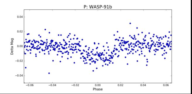
Machine Learning for Transit Detection                      3
firm the source, which makes misclassifications of these ob-         a V-magnitude of less than 12.5. We used only the amalga-
ject types possible. The final categorization (planet, eclips-       mated light curves combined across all cameras and observ-
ing binary, variable, blend, etc) recorded by human vetters          ing seasons for which data was present that were then de-
or observers is known as the disposition.                            trended with a combination of SysRem (Tamuz et al. 2005)
     While effort was taken early in the WASP project to             and the Trend-Filtering Algorithm (TFA; Kovács et al.
standardize individual classifications through training ses-         2005) and searched with a hybrid Box Least-Squares (BLS)
sions and cross validation, the current method of identifying        method (Kovács et al. 2002).
planetary candidates remains partially dependent on indi-                 An initial transit width, depth, period, epoch of mid-
vidual opinions. It would be better to establish a system that       transit, and radius are estimated from the BLS. Stellar fea-
can systematically go through all of the data and identify           tures such as the mass, radius, and effective temperature are
targets, ideally ranked by their likelihood to be genuine plan-      found by the method described by Collier Cameron et al.
ets, derived from the knowledge gained from the entire his-          (2007), in which the effective temperature is estimated from
tory of past dispositions. The past decade of classifications        a linear fit to the 2MASS J − H color index. The main-
and observations has generated a dataset containing both             sequence radius is derived from Teff using the polynomial
descriptions of the target and their classification, creating        relation of Gray (1992), and the mass follows from a power-
an excellent starting point for supervised machine learning.         law approximation to the main-sequence mass-radius rela-
                                                                                    1/0.8
                                                                     tion, M∗ ∝ R∗        . A more rigorous fit to the transit profile
                                                                     yields the impact parameter and the ratio of the stellar ra-
3     METHODS                                                        dius to the orbital separation, and hence an estimate of the
                                                                     stellar density. Markov-chain Monte Carlo (MCMC) runs are
Several classification algorithms were explored with the goal        performed to sample the posterior probability distributions
of reliably identifying planet candidates. We seek to more ef-       of the stellar and planetary radii and orbital inclination.
ficiently use the telescope time for follow-up observations by       The MCMC scheme uses optional Bayesian priors to impose
reducing the number of false positive detections as far as is        a main-sequence mass and radius appropriate to the stellar
reasonable without compromising sensitivity to rare classes          effective temperature. Note that the results and predictions
of planet such as short-period and inflated hot Jupiters.            would change if the precise radius were used instead, partic-
Other goals, such as finding specific subsets of planets with        ularly if the star has evolved off of the main sequence.
higher precision, could be carried out by retraining the al-              In addition to the provided information, we add several
gorithms for that given purpose. In this section we will dis-        new features to capture more abstract or relational infor-
cuss the different machine learning methods utilized and the         mation, such as the ratio of transit depth to width and the
datasets created to train the algorithms.                            skewness of the distribution of the magnitudes found within
                                                                     the transit event. The latter is a possible discriminator be-
                                                                     tween ‘U’ shaped central transits of a small planet across a
3.1    Initial Data Exploration
                                                                     much larger star, and shallow ‘V’ shaped eclipses of grazing
Periodic signals in the lightcurve can come from astrophysi-         stellar binaries. The new high precision distance calculations
cal sources other than transiting planets (Brown 2003). We           released by Gaia (Gaia Collaboration et al. 2016, 2018) are
refer to a periodic dip caused by something other than a             used to measure the deviation of the estimated main se-
planet as an astrophysical false positive. It is essential for any   quence radius calculated as above and the measured radius.
machine learning application to distinguish between plan-            In total, 34 features are included in the dataset. A full list
etary signals and false positives. Fortunately many types            of features and their definitions can be found in Table 1.
of astrophysical configurations have been identified in the               Before training, the full dataset containing the star
WASP archive. The training dataset used for the RFC is               name, descriptive features, and disposition is split randomly
composed of a table of data containing all of the planets            into a training dataset and a test dataset. In total there are
(P), eclipsing binaries, both on their own and blended with          4,697 training cases and 2,314 testing samples. Prior to run-
other nearby objects (EB/Blend), variable stars (V), and             ning the classifiers, all of the features of the training dataset
lightcurves containing no planetary transit after human in-          are median centered and scaled in order to reduce the dy-
spection (X). Blends are especially common in WASP data              namic range of individual features and to improve perfor-
because it has a 3.5-pixel (48 arcsec) aperture, leading to the      mance of the classifier. The scaling parameters are retained
blending of signals from several stars. Is is notable that the       so that they can be applied to subsequent datasets to which
WASP archive labels a planet as ’P’ even if discovered by a          the classification is applied, including the testing dataset.
different survey. While not all of these planets are detectable           The training dataset is used as an input to a vari-
by eye in the WASP data, planets discovered by other in-             ety of classifiers, namely a Support Vector Classifier (SVC;
struments are included in the training sample with the aim           Cortes & Vapnik 1995), Linear Support Vector Classifier
of extending the parameter space to which the classifiers            (LinearSVC), Logistic regression (For the implementation
are sensitive. Low-mass eclipsing binaries (EBLMs) were ex-          is sci-kit learn, see Yu et al. 2011), K-nearest neighbors
cluded from the training and testing datasets, as their signals      (KNN; Cover & Hart 1967), and Random Forest Classifier
look photometrically similar to that of a transiting planet.         (RFC; Breiman 2001). All of the classifiers are run using
However, we do test the final algorithms performance on              the relevant functions in Python’s Scikit-learn package
these objects in section 4.                                          (Pedregosa et al. 2011). The classification algorithms have
     The final size of each of these classes is shown in Fig.        default tuning parameters, but they are not always the best
1. All lightcurves used in this study have been classified by        choice for the given dataset. We therefore vary the param-
members of the WASP team as of August 6, 2018 and have               eters in order to find an optimal combination. While it is

MNRAS 000, 1–15 (2018)
4 N. Schanche et al
Table 1. Features used by the classifiers. Starred features are those added to the dataset, while the rest were taken directly from the
Hunter query. The efficacy of many of these measures for false-positive identification is discussed in detail by Collier Cameron et al.
(2006)
Feature Name Description
clump idx Measure of the number of other objects in the same field with similar period and epoch
dchi P* The ∆χ2 value at the best-fit period from the BLS method.
dchi P vs med* The ratio of ∆χ2 at the best-fit period to median value.
dchisq mr Measure of the change in the χ2 when MCMC algorithm imposes a a main-sequence (MS) prior for mass and radius.
delta Gaia* stellar radius from MCMC - Gaia dr2 radius divided by Gaia dr2 radius
delta m* The difference between the mass calculated by J-H and the MCMC mass.
delta r* The difference between the radius calculated by J-H and the MCMC mass.
depth The depth of the predicted transit from Hunter.
depth to width* Ratio of the Hunter depth and width measures.
epoch Epoch of the predicted transit from Hunter (HJD-2450000.0)
impact par impact parameter estimated from MCMC algorithm.
jmag-hmag Color index, J magnitude - H magnitude.
kurtosis* Measure of the shape of the dip for in-transit data points.
mstar jh Mass of the star, from the J-H radius*(1/0.8).
mstar mcmc Stellar mass determined from MCMC analysis.
near int* Measure of nearness to integer day periods, abs(mod(P+0.5,1.0)-0.5).
npts good Number of good points in the given lightcurve.
npts intrans Number of datapoints that occur inside the transit.
ntrans Number of observed transits.
period Detected period by Hunter? in seconds.
rm ratio* Ratio of the MCMC derived stellar radius to mass.
rplanet mcmc Radius of the planet, from MCMC analysis.
rpmj Reduced proper motion in the J-band (RPMJ=Jmag+5*log10(mu)).
rpmj diff Distance from DWs curve separating giants from dwarfs.
rstar jh Radius of the star derived from the J-H color measure.
rstar mcmc Radius of the star determined from MCMC analysis
sde Signal Detection Efficiency from the BLS.
skewness* Measure of the asymmetry of the flux distribution of data points in transit.
sn ellipse Signal to noise of the ellipsoidal variation.
sn red Signal to red noise.
teff jh Stellar effective temperature, from J-H color measure.
trans ratio Measure of the quality of data points (data points in transit/total good points)/transit width.
vmag Cataloged V magnitude.
width Width of the determined transit in hours.
impractical to test every possible combination of parame- sification. The exception is the SVC, which shows a sharp
ters, we ran a grid of tuning parameter combinations spe- decrease in false positives while the true positives and true
cific to each classification method to find the optimal settings negatives remain the same.
for the final algorithm. The results using the best perform-
ing parameters for each method are reported in Table 2. A
more detailed description of what each parameter does can 3.2 Random Forest Classifiers
be found in the documentation for Scikit-learn 2 .
Several of the classifiers, and particularly the K-nearest After exploring several different classification techniques, we
neighbor classifier, show poor performance using the training decided to pursue the RFC in more detail because of its high
data because the class of interest, the planets, is underrep- recall rate (See Table 2). RFC is one of the most widely
resented in the dataset. To try to compensate for this, we used machine learning techniques, and is particularly useful
also try adding additional datapoints using the Synthetic in separating data into specific, known classes. Applications
Minority Over-sampling Technique (SMOTE; Chawla et al. to astronomy include tracking the different stages of individ-
2002). This technique creates synthetic datapoints for the ual galactic black hole X-ray binaries by classifying subsec-
minority classes that lie between existing datapoints with tions of the data (Huppenkothen et al. 2017), classifying the
some added random variation. The synthetic data is added source of X-ray emissions (Lo et al. 2014), and distinguishing
only to the training data, and the test dataset remains the between types of periodic variable stars (Masci et al. 2014;
same as before. The addition of SMOTE data generally in- Rimoldini et al. 2012).
creased the number of planets retrieved from the data, but RFC has many advantages, most notably the ease of im-
also increased the number of non-planets given a planet clas- plementation, solid performance in a variety of applications,
and most importantly for our study, the easily traceable de-
cision processes and feature ranking. It is because of this last
2 http://scikit-learn.org/stable/ advantage that we focus our attention on the RFC over the
MNRAS 000, 1–15 (2018)Machine Learning for Transit Detection 5
Classifier TP FP FN Precision Recall F1 Accuracy Tuned Parameters
LinearSVC 35 83 13 30 73 43 80 C=60, tol=0.0005
SVC 37 46 11 45 77 57 82 kernel=’rbf’, C=12, gamma=0.03
LogisticRegression 34 76 14 31 71 43 81 C=90, tol=0.005
KNN 5 4 43 56 10 17 81 n neighbors=15, weights=’distance’
RandomForest 44 125 4 26 92 41 79 n estimators=200, max features=6, max depth=6
LinearSVC* 44 142 4 24 92 38 76 C=20, tol=0.0002
SVC* 36 37 12 49 75 59 81 kernel=’rbf’, C=25, gamma=0.02
LogisticRegression* 42 128 6 25 88 39 78 C=60, tol=0.0006
KNN* 45 151 3 23 94 37 74 n neighbors=7, weights=’distance’
RandomForest* 45 137 3 25 94 39 78 n estimators=200, max features=6, max depth=6
Table 2. Results of the classification algorithms, trained on 4,697 samples. The results here are reported for the 2,314 samples making
up the test dataset. We report here the planets correctly identified (True Positives - TP), non-planets incorrectly labeled as planets
(False Positives - FP) and the number of planets missed by the algorithm (False Negative - FN). From this we calculate the precision
(TP/(TP+FP)), recall (TP/(TP+FN)), and F1 score (F1 = 2*Precision*Recall/(Precision + Recall)) for the planets. The accuracy
reflects the performance of the classifier as whole, and shows the total number of correct predictions of any label divided by the total
number of samples in the test dataset. The full confusion matrix for all of the classifiers reported here can be found as an appendix in the
online journal. The Tuned Parameters column reports the best performing values for the listed parameters, as determined by using the
GridSearchCV function, which tests all combinations of a specified grid of parameters. Classifiers marked with an * use a training sample
that added training examples using SMOTE sampling, explained more fully in text. By adding SMOTE datapoints, the training set
grew to 10,672 samples, while the testing dataset remained the same. The Linear SVC, SVC, and Logistic Regression Classifier that did
not use the SMOTE datapoints are run using the keyword class weight=’balanced’, which weights each sample based on the number of
entries in the training dataset with that label. The Random Forest classifier without SMOTE resampling uses the class weight keyword
’balanced subsample’, which has the same function but is recomputed for each bootstrapped subsample. While the SVC both with and
without the SMOTE training sample performed very well in the ’f1’ score and overall accuracy, the false negative rate was higher than
desired for practical application. The RFC showed the highest recall, which we want to maximize to find the widest range of planets. We
therefore prefer the RFC, with a trade-off of having more false positives that would be flagged for follow-up.
linear SVC, SVC, linear regression, or KNN methods. RFC is tree was capped at a depth of 6 and allowed 6 random fea-
an ensemble method of machine learning, comprised of sev- tures at each split in the tree, which helps to reduce overfit-
eral individual decision trees. Each decision tree is trained ting.
on a random subset of the full training dataset. For each One advantage of the RFC method is that many differ-
‘branch’ in the tree, a random subset of the input charac- ent features can be included, and not all features need to be
teristics known as ‘features’ are selected and a split is made effective predictors. This can be useful for exploratory data
based on a given measure that maximizes correct classifica- analysis as the user can include all of the various data el-
tions, with samples falling above and below the split point ements without introducing biases from curating the input
moving to different branches. Each branch then splits again list. Conversely, it is important to note that the performance
based on a different random subsample of features. This con- of the RFC depends on the quality of the input features. It is
tinues until either all remaining items in the branch are of possible that the performance of all classifiers could increase
the same classification or until a specified limit is reached. if better features are identified.
The output of the RFC is a fractional likelihood that the in-
put object falls into each category, and the highest likelihood As a byproduct of the training process, the RFC can
is then used as the classification. analyze the importance of the various features in making
predictions. The results of such an analysis using our train-
On its own, each decision tree does not generalize well ing dataset are shown in Fig. 2. This can be used to gain in-
to other datasets to make predictions. However, by training sight into the decision making process that the classifier has
many different trees and combining them to use the most developed, which can inform further analysis. For example,
popular vote as the prediction, a more successful and gen- the period of the planet was the strongest indicator. This
eralized predictor is created. There are many ways to tune can be explained in large part because false planet detec-
the RFC to try to optimize the classification for the dataset. tions arising from diurnal systematics tend to have orbital
For example, the number of trees in the forest, the depth of periods close to multiples of one sidereal day due to the
the tree (the number of splits that can be performed), the day/night cycle present in Earth-based observations. This
number of features available at each split, and the method indicator would likely not play as significant a role in a space-
used to optimize the splits are all characteristics that can be based survey unaffected by the day/night cycle. The width
modified. There is no set rule for choosing these parameters, or duration of the transit, estimated radius of the planet, the
and therefore many different tests are conducted to try to ∆χ2 value (a product of the BLS search) of the object at
optimize the results. Here, we use Scikit-learn’s Random- the best-fit period, and the number of transits of the object
ForestClassifier method to perform the classification and to round out the top 5 features in prediction.
tune the parameters. We find that the highest-performing The features that had relatively little impact on the
forest contains 200 trees, above which the accuracy increased overall prediction related largely to stellar properties, in-
very minimally for the increased computation time. Each cluding the magnitude and radius of the star. This shows
MNRAS 000, 1–15 (2018)6 N. Schanche et al
3.3 Neural Networks
The past decade has shown an explosion of new applications
EB/Blends of Neural Networks to tackle a variety of different problems.
The particular flavor of neural networks is dependent on the
specified task at hand and the types of data available for
56.3%
training. The basic idea of a Neural Network was originally
inspired by the neurons in a human brain, although in prac-
tice artificial neurons are not directly analogous. Nonethe-
less, like the human brain, this type of structure is useful for
learning complex or abstract information with little guid-
ance from external sources. In the following section, we dis-
cuss Convolutional Neural Networks (CNN) and their appli-
2.2%
18.6% cation to the WASP database.
P
X
23.0%
3.3.1 Convolutional Neural Networks
V A standard Artificial Neural Network (ANN) has the basic
structure of an input layer containing the features of the in-
put data, one or more hidden layers where transformations
are made, and the output layer which offers the classifica-
tion. The output of each layer is transformed by a non-linear
activation function. The basic building-blocks of ANNs are
Figure 1. Pie plot showing the relative number of examples for known as neurons. A basic schematic of the system archi-
planets (P), eclipsing binaries and blends (EB/Blends), variable tecture is shown in Fig. 4.
stars (V) and lightcurves otherwise rejected as planet hosts (X). In this work, we use the Keras package (Chollet et al.
This represents an unbalanced dataset, with the smallest class be- 2015) to implement the neural network, which offers a vari-
ing the class of special interest, planets. In real life, there are more ety of built-in methods to customize the network. At each
non-detections (X) than the other classes. However, the training layer, the input data is passed through a non-linear activa-
data is composed of lightcurves that have been manually identi- tion function. Many activation function choices are available,
fied and flagged. Many non-detections are simply ignored by ob-
but here we choose the rectified linear unit, or ’relu’ func-
servers rather than labeled X, leading this class to be smaller than
expected. The mismatched sample size is important in machine
tion (Nair & Hinton 2010) for all layers except the output
learning, as considerations must be taken to bring representation layer, to which we instead apply a sigmoid function. The relu
to the minority classes. function was chosen both because of its wide use in many
applications and because of its high performance during a
grid search over our tuning parameters. In addition to the
activation function, each neuron is assigned a weight that is
applied to the output of each layer, and is modified as the
that there is no strong preference for a certain size star to algorithm learns. Using Keras, we tested a random normal,
host a particular type of object in our sample, as the ap- a truncated normal distribution within limits as specified
parent magnitude range to which WASP is most sensitive by LeCun (LeCun et al. 1998), and a uniform distribution
is dominated by F and G stars (Bentley 2009). The lowest within limits specified by He (He et al. 2015) initialization
ranked feature is the skewness, showing that the asymmetry of the weights and found the greatest performance with He
of datapoints falling within the best-fit transit is not suffi- uniform variance scaling initializer.
ciently capturing the transit shape information. The learning itself is managed using the Adamax opti-
The results of the RFC, shown in Fig. 3, show that mizer (Kingma & Ba 2014), a method of optimizing gradient
∼93% of confirmed planets are recovered from the dataset. descent. In gradient descent, classification errors in the final
The ones that are not recovered are most often rejected with output layer are propagated backwards through the network
the label ’X’. The more concerning statistic is that more than and the weights are adjusted to improve the overall error
10% of EB/Blends were misclassified as planets. Since there during the next pass through the network. This is an iter-
are far more binary systems recorded than there are planets, ative process, with small adjustments made after each pass
this quickly turns into a large number of lightcurves incor- through the network until a minimum error (or maximum
rectly identified, which translates to many hours of wasted number of iterations) is reached. The maximum change in
follow-up time. For our testing dataset, there are 45 correct the weights allowed by Adamax at each iteration is con-
planet identifications and 137 that are false positives. This trolled by the learning rate, which can be tuned to different
means that if all objects flagged as planets are followed up values for individual datasets. Finally, at each stage, we in-
on, we would expect about 25% of them to be planets. In corporate neuron dropouts, where a fraction of the neuron
reality, not all flagged objects are good candidates and can inputs are set to 0 in order to help prevent overfitting. The
be eliminated by visual inspection. Regardless, the high false total dropout percent is determined experimentally, and here
positive rate led to the development of Convolutional Neural we find 40% to be effective.
Networks as a secondary test on the lightcurves, as discussed While the numerical data used in the RF could be
in 3.3.1. passed to the neural network directly, this data only pro-
MNRAS 000, 1–15 (2018)Machine Learning for Transit Detection 7
Relative Importance of Each Feature
period
width
rplanet_mcmc
dchi_P_vs_med
ntrans
depth_to_width
dchi_P
clump_idx
depth
sn_ellipse
sde
near_int
npts_intrans
trans_ratio
delta_Gaia
sn_red
epoch
Features
npts_good
delta_m
kurtosis
rpmj_diff
dchisq_mr
rm_ratio
delta_r
mstar_jh
teff_jh
rstar_mcmc
rstar_jh
rpmj
jmag-hmag
impact_par
vmag
mstar_mcmc
skewness
0.00 0.02 0.04 0.06 0.08 0.10 0.12 0.14
Relative Importance in the Random Forest
Figure 2. Ranked list of the effectiveness of each of the features in making correct classifications of the training dataset for the Random
Forest Classifier. Properties of the transit itself, such as the period and width, are shown to be important discriminators in identifying
genuine transits, while stellar properties like magnitude and mass are not effective for classification.
vides insight into the statistical distribution of the classes, be of the same length. To standardize the data length, the
producing results similar to that of the RFC. In practice, it folded lightcurves are divided into 500 bins in transit-phase
can be the case that many of the features fall within the right space. The number of bins was determined experimentally,
range to be labeled with a certain class, but a quick visual with 500 being the best trade off between providing detailed
inspection of the lightcurve can easily rule the classification lightcurves without having a significant number of bins miss-
out. Instead it would be desirable to create an algorithm ing data.
that can use the shape of the lightcurve itself to make clas- Once the data are binned, a set of one-dimensional con-
sification decisions. Using the lightcurve data would more volution filters are passed over each lightcurve. This has the
closely mimic the human process of eyeballing. effect of making our dataset larger by a factor of the number
In order to directly use the lightcurve data, we devel- of filters, so to reduce the data size and help prevent over-
oped a Convolutional Neural Network (CNN; LeCun et al. fitting we apply a MaxPooling layer where we only keep the
1990; Krizhevsky et al. 2012). In this case, the input data we maximum value of every n data points. Finally a dropout
use is the actual magnitude measurements of WASP folded layer is added, in which a random specified fraction of the
on the best-fit period determined by the BLS. In the CNN points are ignored to prevent overfitting the training data.
that we adopt, the magnitude data first undergoes a series We then repeat this entire process to add more complex and
of convolution steps, in which various filters are applied to abstract filters. Finally, all of the remaining data is flattened
the data to enhance defining characteristics and detect ab- so that each lightcurve, now comprised of several filtered
stracted features. The filters themselves are optimized itera- and pooled representations of the original lightcurve, are
tively to find those that best enhance the differences between added together to make a one dimensional array for each
classes, similar to the way the weights between the neural star, which is then passed into the fully connected layers
layers are updated. The convolution process is represented of the neural network. All of the layers of the network are
in Fig.5. optimized to provide the best fit to the data in the final
Each WASP field contains a different number of sample classification layer.
points, yet input to the CNN for all of the samples need to The training set is highly unbalanced with relatively
MNRAS 000, 1–15 (2018)8 N. Schanche et al
EB/Blend Percent Correct Predictions True Number Correct Predictions
EB/Blend
68.2602 10.2665 15.9091 5.56426 871 131 203 71
2.08333 93.75 2.08333 2.08333 1 45 1 1
WASP disposition
WASP disposition
P
P
4.15879 0.378072 91.6824 3.78072 22 2 485 20
V
V
1.51844 0.867679 8.67679 88.9371 7 4 40 410
X
X
EB/Blend P V X EB/Blend P V X
Predicted class Predicted class
Figure 3. Confusion matrix showing the results of the RFC using the training dataset containing synthetic datapoints generated through
SMOTE sampling. The x-axis indicated what the algorithm predicted and the y-axis displays the human labeled class, which we assume
to be accurate. Correct predictions fall on a diagonal line from upper left to lower right. The plot on the left shows the results as a
fraction of lightcurves that fall into that bin. However, since the number of samples in each class varies, a more practical depiction is
shown in the right plot, which shows the actual number of lightcurves for each category.
started with all X stars and measured the RMS against the
V-magnitude. Those objects that fell more than 1σ below
the best fit to the data were selected, as they show the least
amount of variation. This left a total of 848 light curves.
The planetary signal added to the WASP data was
created using the batman package for Python (Kreidberg
2015). The stellar mass, radius, and effective temperature
are set using the known values for the star itself. The plane-
tary properties were generated randomly with the following
distributions.
The period was randomly selected to be a value uni-
formly located in log space between 0.5 and 12 days, as this
is the range in which the WASP pipeline typically uses the
BLS algorithm to look for planets. The mass of the planet
follows the same lognormal distribution used in Cameron &
Jardine (2018), with a mean of 0.046 and a sigma value of
Figure 4. Visual representation of a neural network scheme, .315. The semi-major axis can be found for the period using
where circles represent individual neurons. In this example, the
layers progress from top to bottom. The top row represents the in-
put layer, followed by 2 hidden layers, and finally an output layer,
where the class prediction is made. Circles with crosses through p2 G(M1 + M2 ) 13
a=( ) (1)
them represent dropped neurons, described further in text. 4π 2
The radius of the planet is dependent on both the mass
few planets as compared to eclipsing binaries and blends, of the planet and the equilibrium temperature. We use a
variables, or lightcurves with no signal, which limits the cubic polynomial in log mass and a linear term in log effec-
performance of the CNN. To compensate, we extended the tive temperature to approximate the planetary radius, using
sample of ’P’ training examples by creating artificial transit coefficients derived from a fit to the sample of hot Jupiters
lightcurves. studied by Cameron & Jardine (2018):
The lightcurve injection was done by adding synthetic
transit signals to existing WASP light curves that showed
no transit signal or other variability. This ensured realis-
2
Rp Mp Mp
tic sampling and typical patterns of correlated and uncorre- log = c0 + c1 log + c2 log
RJup 0.94MJup 0.94MJup
lated noise. We began with a sample of lightcurves of objects 3 T 4
classified as ’X’ in the Hunter catalog, meaning they have Mp eql
+c3 log + c4 log , (2)
been rejected and contain no detectable planet signal. We 0.94MJup 1471 K
MNRAS 000, 1–15 (2018)Machine Learning for Transit Detection 9
The lightcurves were generated and added to one of the
selected WASP lightcurves folded on the assigned period.
While some of these new planets were too small to be visible,
and others were much larger than would be expected, we
chose to include them all in order to push the boundaries of
the parameter space that the CNN is sensitive to so as not
to exclude potentially interesting, though unusual, objects.
The lightcurves of the artificial planets, as well as real-
data examples of P’s, EB/Blend’s, V’s, and X’s are phase
folded on the best-fit period (or assigned period, in the case
of the artificial planets) and binned by equal phase incre-
ments. Including the artificial planets, there are 4,627 ob-
jects in the training set and 2,280 in the testing dataset.
The CNN parameters were set by using a grid search
over the tunable parameters. The final CNN was comprised
of two convolutional layers with 8 and 10 filters respectively.
The pooling stages each had a size of two, and 40% of the
neurons were dropped at each set. The flattened data were
passed to a neural network with two hidden layers of sizes
512 and 1048 and with a ’relu’ function. Both of these layers
also had a 40% dropout applied. The learning rate for the
Adamax optimizer was 0.001. The most effective batch size
was 20 with 225 total epochs. As with the RFC, the out-
put of the CNN is a likelihood that the lightcurve falls into
each of the categories, with the highest likelihood being the
prediction.
Using only the binned lightcurve as input, the CNN
achieves an overall accuracy (correct predictions divided by
Figure 5. Simplified visual representation of the convolution
total lightcurves analyzed) of around 82% when applied to
steps for a full lightcurve, folded on the best fit period. The shad-
ing of the boxes represents the different filters that are applied the test dataset. While the fraction of correctly identified
to the data in each step. Also at each convolution step, the data planets is lower than the RF (88% as opposed to 94%), the
length is reduced using the Max Pooling method, in which only CNN performs much better in classifying eclipsing binaries
the maximum value of every n datapoints is kept. In the final and blends in terms of the percent of false positives with only
step, all of the pooled and filtered data are stacked one after the ∼5% of EB/Blends being labeled as planets, as opposed to
next. This new one-dimensional dataset is then passed into the 10% for the RF. The CNN therefore has an overall better
fully connected layers of the neural network. The final network ar- performance for follow-up efficiency.
chitecture is as follows: the input data is comprised of one dimen- In order to further increase the performance of the
sional magnitude data binned to length 500. The first convolution
CNN, we train a second CNN algorithm to include the lo-
step has 8 filters with a kernel size of 4. The data is then pooled
by 2. Each lightcurve at this point has 8 layers of length 250. The
cal transit information, using an approach similar to that
second convolution step has 10 filters with a kernel size of 8, fol- of Shallue & Vanderburg (2018). The local information is
lowed again by another pooling layer with a pool size of 2 leading comprised of the data centered on the transit and only con-
to a datasize of 10 layers of length 125. The information from all taining the data 1.5 transit durations before and after the
of the filters is then flattened into one layer of length 1,250 for transit event, standardizing the transit width across events.
each lightcurve, and is input to the first densely connected layer. An example of a local lightcurve is shown in Fig. 6. The
There are 2 dense hidden layers of size 512 and 1024. Each stage effect of this is to provide greater detail and emphasis on
of the convolution and fully connected layers has a 40% dropout the shape of the transit event itself in order to understand
rate to prevent overfitting. The final output layer has 4 neurons, the subtle shape difference between a typical planet and an
one for each classification category. The CNN with both the full
eclipsing binary system. The full lightcurve and the local
and local lightcurve has the same general format, but with the
input data being a stack of two 500-length lightcurves.
view are stacked and passed together into the CNN. In this
case, the overall accuracy (83%) remained roughly the same,
but the total percentage of planets found increased to (94%).
The trade-off is a slight increase of the number of EB/Blends
where c0 = 0.1195, C1 = −0.0577, c2 = −0.1954, c3 =
1 being labeled as planets. A full comparison of both methods
0.1188, c4 = 0.5223, and Teql = Tef f R2aS 2 can be seen in Fig. 7.
As we are looking only for close-in planets, we make the It is important to note that the way missing data was
simplification that all eccentricities are 0. Finally, the incli- handled for both the full lightcurve and the local lightcurve
nation was calculated by first randomly picking an impact made a large difference in the final performance. When bin-
parameter, b, between 0 and 1. The inclination was then ning the data, the full dataset was evenly split in 500 equal
calculated by phase steps and all of the datapoints within those phase
steps were averaged. In some cases, for example when the
bRS
lightcurve was folded over an integer day, there were gaps
i = cos−1 (3) in the phase ranges in which no data were present. Since
a
MNRAS 000, 1–15 (2018)10 N. Schanche et al
CNN Confusion Matrix (fraction) CNN Confusion Matrix (actual)
EB/Blend
EB/Blend
82.1497 4.51056 7.96545 5.37428 856 47 83 56
WASP disposition
WASP disposition
8.43373 88.253 0.301205 3.01205 28 293 1 10
P
P
7.50507 0 87.2211 5.27383 37 0 430 26
V
V
10.8959 5.56901 12.8329 70.7022 45 23 53 292
X
X
EB/Blend P V X EB/Blend P V X
Predicted class Predicted class
CNN Confusion Matrix (fraction) CNN Confusion Matrix (actual)
Figure 6. A local view of WASP-91b, the same planet as shown
EB/Blend
EB/Blend
81.8182 6.15836 8.01564 4.00782 837 63 82 41
in the CNN example (Fig. 5). This local view was used as an
additional layer in the second CNN. The local version clearly
WASP disposition
WASP disposition
3.35366 94.2073 0.609756 1.82927 11 309 2 6
shows more detail on the transit shape, and specifically the flat-
P
P
bottomed transit. EB/Blends tend to have a ’V’ shape with
steeper sides, which is more apparent in this close-up view. 8.36735 0.204082 88.7755 2.65306 41 1 435 13
V
V
10.0228 8.65604 12.0729 69.2483 44 38 53 304
X
X
the CNN can not handle missing data in the input string, EB/Blend P V X EB/Blend P V X
a value needs to be inserted. We tried inserting either a Predicted class Predicted class
nonsense value, in this case 0.1 which is far above any real
datapoint, or repeating the last good value. In some cases
there were several phase steps in a row that were missing Figure 7. Confusion matrix showing the results of the CNN using
data, causing a small section of the lightcurve to be flat. only lightcurves folded on the best-fit period (top) and with the
After trying both options, we found that by far the best addition of the local transit information (bottom) as input. The
performance was obtained when inserting the nonsense value axes are interpreted the same as in Fig. 3. The plot on the left
into the full lightcurve and repeating the last good value into shows the results as a fraction of lightcurves that fall into that
bin. The right plot shows the actual number of lightcurves for
the local lightcurve. This makes sense, as the full lightcurve
each category. Note that in this example, we artificially injected
gives a broader view of the star’s lightcurve and is likely to additional planets into WASP data to increase the sample, so the
have regular gaps in the data when it is folded on a bad numbers reported are for a combination of the real and artificial
period. The algorithm was able to identify that pattern and planets.
reject it. The local data, however, have fewer total data-
points because they cover a smaller total range of phases,
and therefore are more likely to randomly have missing data.
The algorithm is no longer able to distinguish lightcurves many cases, the blended stars look very similar to planets
missing data because of an intrinsic problem with the data by their numerical descriptors, and in particular the depth
fold and those missing data simply because they lack enough of the transit and the distribution of transit durations look
observations during the transit, confusing the results. very plausible. Without looking at the nearby stars, these
objects are very hard to distinguish.
The CNN has a fundamentally different method of iden-
tifying transits. As described in section 3.3.1, the CNN is
4 ANALYSIS AND RESULTS
not provided with derived data, but rather has direct ac-
When looking at the results of the RFC and CNNs, the per- cess to the magnitude data folded on the best-fit period. In
centage of correct predictions across methods is consistent, this case, the algorithm is simply trying to pattern-match to
with ∼ 90% of planets being correctly identified. However, find the correct shape for a transit. Looking at the true pos-
when looking at the original lightcurves for both true posi- itives and false negatives (examples shown in Fig. 9) for this
tives and false negatives, clear patterns in the different ma- subsection of data shows a different failure mechanism for
chine learning methods begin to emerge. wrongly-identified planets. In many cases, light curves will
The RFC uses features that are derived from the fit- look like planets, but when other information, such as the
ted light-curve parameters and external catalog information, depth of the transit, is known it becomes clear that the ob-
but the lightcurves themselves are not included. This logi- ject is more likely an eclipsing binary or other false positive.
cally leads to candidates that have typical characteristics of In addition, fainter objects tend to have much noisier data
known exoplanets to emerge. However, because the WASP and more sporadic signals, which can sometimes look like
data can be very noisy and have large data gaps, there are a transit signal when the data is binned down to 500 data
many occasions where the derived ’best fit’ planet features points. Finally, the drift of stars across the CCD during each
fall into the known distribution, but upon inspecting the night can lead to systematic disturbances that are consistent
original data it is clear that there is no periodic transiting at the beginning or end of each night in some (but not all)
signal. Examples of true positive and false negative classifi- target stars. Since this effect is specific to each star, it is
cations for the RFC are shown in Fig. 8. The main contrib- not always corrected by decorrelation. This can lead to the
utors of false positives for the RF is the blended star (rather lightcurve having a clear drop in magnitude at regular inter-
than the eclipsing binary) component of the EB/Blends. In vals, and the gaps in the data can appear transit-like to the
MNRAS 000, 1–15 (2018)Machine Learning for Transit Detection 11 Figure 8. Confusion matrix of RFC results showing examples of lightcurves selected from samples that fall into each category, chosen to represent typical failure modes. Lightcurves along the diagonal, shown in black, were correctly classified by the RFC. Off diagonal boxes, shown in gray, were incorrectly identified, with the true classification shown on the vertical axis and the predicted classification shown on the horizontal axis. Looking at the samples in the off-diagonal boxes provide insight into how the RFC makes its decisions and what the common failure modes are. SW1832+53 was labeled as an X in the archive, but the RF predicted it was a variable object. This classification was made early in WASPs’ history, and a clearer picture of the lightcurve has since been established. While an X classification means that there is no planetary signal, a better classification for the object would be to label it as a variable lightcurve, which is what the random forest does. SW0826+35 is another interesting object. It was labeled as a variable in the archive, but the alternating depths of dips indicates it may actually be an eclipsing binary, consistent with the machine classification. The final object of special note is SW0146+02, verified as WASP-76b. This planet’s transit is particularly deep and confused the RFC into mislabeling it as an EB/Blend showing that this algorithm is sensitive to the depth of transit despite the classical ’U’ shape of the event. MNRAS 000, 1–15 (2018)
12      N. Schanche et al

Figure 9. Same as for Fig. 8, but for the CNN using the local and full binned lightcurve. As in the RFC, the overlap in categories in
the human classifications is evident in the CNN results. For example, SW1924-33 was labeled by a WASP team member as an X because
it does not contain a planetary transit, but it clearly does show a transit event and therefore could be instead classified as an eclipsing
binary. While this is considered a wrong classification in the algorithm evaluation, in practice it is an acceptable output. SW1308-39 is an
example where near-integer day (in this case near 11 days) effects can look like transit signals when the data is phase binned. The CNN
did miss several true planets, such as SW1303-41 (WASP-174b; Temple et al. 2018), as the dip is very small with a messy lightcurve.
SW1521-20 is an example of a planet found in a different survey (EPIC 249622103; David et al. 2018) with the signal not being visible
in the WASP data.

                                                                                                                MNRAS 000, 1–15 (2018)
Machine Learning for Transit Detection 13
CNN. Interestingly, this last problem is far more prevalent low-mass eclipsing binary systems, 92 (23%) were classified
when fewer neurons in the ANN are used. Increasing the as planets. The CNN with only the full lightcurve also re-
neurons to 512 and 1024 in our final configuration nearly turned 64 as planets, partially overlapping with the RFC
eliminates the problem, although a few cases do still get predictions. Adding the local lightcurve information made
through. the CNN more likely to identify EBLMs as planets with 95
(24%) being labeled as planets. The SVC is the most shrewd,
with only 24 stars labeled as planets. For many of these ob-
jects, the transit signals look identical to those of planets
5 DISCUSSION and are only discovered with follow-up information. Even
Each of the machine learning methods above performs best by combining results from different machine learning meth-
on a specific subset of planets. Like a human looking at a ods, we expect to have many of these type of objects flagged
list of transit properties, the RFC and SVC are better suited for further observation, reducing the overall performance of
to finding planets that have strong signals and have prop- the algorithms.
erties similar to those of the other known WASP planets. There are several caveats to our study. One note of cau-
The CNN using the magnitude data folded on the best fit tion is the underlying training dataset. The training data
period functions similar to a human eyeballing a lightcurve was obtained by combining the entries of a number of WASP
and making decisions. By combining the predictions of these team members over the course of many years. This leads to
methods, we get a more robust list of planetary candidates. two main problems. First, different team members may label
The importance of the combination of machine learning al- the same lightcurve differently based on their interpretation.
gorithms has also been noted by others (Morii et al. 2016; Blends and binaries for example can be used differently by
D’Isanto et al. 2016), and will be an important framework different users. We attempted to control for this by manu-
for upcoming large-data surveys. ally inspecting the blends and binaries and updating flags
Currently, radial velocity follow up of WASP targets to maintain consistency across all fields. The ’X’ category
takes place primarily using the CORALIE spectrograph at is also notably inconsistent, with objects that were rejected
the La Silla Observatory in Chile (Queloz et al. 2000) for as planets for many different reasons, including blends and
southern targets and the Spectrographe pour lâĂŹObserva- binaries, being given the same label.
tion des PhÃl’nomÃĺnes des IntÃl’rieurs stellaires et des Ex- The second issue comes from the fact that the classifica-
oplanÃĺtes (SOPHIE; Perruchot et al. 2011) at the Haute- tion began before all current data were available. After the
Provence Observatory located in France for targets in the first few WASP observing seasons, classifications were made
north. based on the limited data available. When other data were
Since thorough records have been kept of the WASP added in the following seasons, the shape of the lightcurve
follow-up program with CORALIE, 1234 candidates have may have changed and more (or less) transit-like shapes be-
been observed and dispositioned. Of those, 150 (12%) have came obvious. However, since the candidate was already re-
been classified as planets (2 of which are the brown dwarfs jected, it was never re-visited and updated. Several examples
WASP-30 and WASP-128), 713 (58%) are binaries or blends, like this were found by looking through the incorrect classi-
225 (18%) were low mass eclipsing binaries, and the remain- fications, such as those in Figures 8 and 9, and remained un-
ing 146 (12%) were rejected for other reasons, including 60 corrected in our training data. Regardless of these problems,
because the stars turned out to be inflated giants. The SO- the algorithms were robust and were able to make reasonable
PHIE follow-up effort has a similar success rate to date. Of predictions even with small variations in the training.
the 568 total candidates dispositioned, 53 (9%) are planets, Finally, we rely on the BLS algorithm to provide an ac-
323 (57%) are blends or binaries, 116 (20%) were low-mass curate best-fit period. This is especially important for the
eclipsing binaries, 72 (13%) were rejected for other reasons CNN, which only has the lightcurve folded on that period
including being a giant star, and 4 (1%) were variable stars. as input. The CNN is therefore not equipped to handle pos-
As a comparison, for our RFC, 182 objects were classi- sible incorrect periods due to aliases or harmonics. It would
fied as planets, with 45 true positives and 137 false positives, be possible to augment the code to also include other infor-
indicating a success rate of 25%. The SVC is more conser- mation for the CNN, such as the data folded on half of the
vative, finding fewer total planets but rejecting more false period and twice the period, either in a stack or as a sepa-
positives, and has a 49% estimated follow-up accuracy (True rate entry, to try to identify planets in the data that were
positives divided by true positives and false positives). The found at the wrong period. This possibility will be included
CNN with the full lightcurve showed even better results, in future work, but is beyond the exploratory scope of this
with 81% estimated follow-up accuracy, and when the lo- paper.
cal lightcurve data was added 75% of the objects flagged as The classifications shown here have a lower accuracy
planets were true positives. It may seem like the CNN would than those reported in the Kepler studies, which range from
be the best option to use alone, but it did miss several plan- around 87% up to almost 98%. This is to be expected, as
ets that the RFC was able to recover and occasionally let WASP data is unevenly sampled and has much larger mag-
in false signals that were caught by the RFC or SVC, high- nitude uncertainties, making definitive identifications im-
lighting the importance of combined methods. possible with WASP data alone. WASP’s large photomet-
We note that the true follow-up rate for any of these ric aperture (48 arcseconds) also makes convincing blends
methods would be lower in practice. Eclipsing binaries with more common. Nevertheless, the machine learning algo-
low-mass stellar companions, which closely resemble plan- rithms were able to correctly identify ∼90% of planets in
ets in their lightcurves and derived features, were removed the testing dataset and operate much faster than human
from the training dataset. When we applied the RFC to 399 observers (less than 1 minute to train the RFC and around
MNRAS 000, 1–15 (2018)You can also read