Static and Dynamic Input-Output Modelling with Microsoft Excel - Anett Großmann, Frank Hohmann (GWS)
←
→
Page content transcription
If your browser does not render page correctly, please read the page content below
SHAIO CONFERENCE PAPER 2019

Static and Dynamic Input-Output
Modelling with Microsoft Excel

Anett Großmann,
Frank Hohmann (GWS)
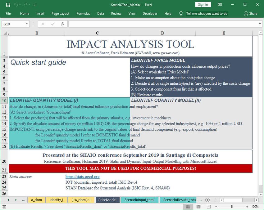
TABLE OF CONTENTS

Figures                                                        3

Abstract                                                       4

1    Introduction                                              5

2    Static Input-Output Models                                6
    2.1 Overview                                               6
    2.2 Implementation into MS Excel                           7
        2.2.1 Leontief Quantity Model                          8
        2.2.2 Leontief Price Model                             11
        2.2.3 Scenario Analysis                                15
    2.3 Conclusions                                            16

3    Dynamic Input-Output Model (DIOM-X)                       16
    3.1 Overview                                               16
    3.2 Technical Foundation                                   18
        3.2.1 Essential Programming Language Features          18
        3.2.2 Excel VBA Language and Programming Environment   20
    3.3 Steps in Model Building                                21
    3.4 Implementation into MS Excel                           24
        3.4.1 Data Management                                  24
        3.4.2 Regression Analysis                              27
        3.4.3 Core Model Framework                             30
        3.4.4 Model Template and its Implementation in VBA     32
        3.4.5 Scenario Analysis                                37
    3.5 Conclusions                                            39

4    Summary and Outlook                                       40

References                                                     41

                                                               2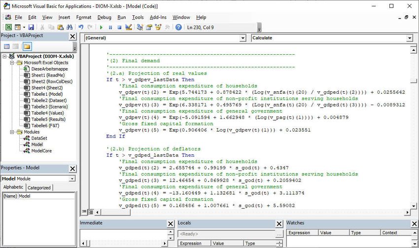
FIGURES

Figure 1:    Static Impact Analysis Tool                                         8
Figure 2:    MS Excel: name manager                                              9
Figure 3:    Leontief quantity model: calculating input coefficients for domestic
             intermediates by using defined names and array formula               9
Figure 4:    Leontief quantity model: Scenario input sheet                      10
Figure 5:    Leontief quantity model: scenario results sheet                    10
Figure 6:    Leontief price model: input and result sheet (I)                   11
Figure 7:    Creating a list in MS Excel                                        12
Figure 8:    Leontief price model: input and result sheets (II)                 13
Figure 9:    Leontief price model: input and result sheets (III)                14
Figure 10:   Leontief price model: input and result sheets (IV)                 14
Figure 11:   Leontief price model: input and result sheets (V)                  15
Figure 12:   Simplified illustration of a dynamic IO model Source: own
             illustration                                                       17
Figure 13:   MS Excel: VBA programming environment                              21
Figure 14:   Comparing scenarios                                                24
Figure 15:   Worksheets Dataset and RowColDesc                                  25
Figure 16:   Values worksheet with data                                         26
Figure 17:   Regression example I                                               28
Figure 18:   Implementing regressions into the VBA code I                       28
Figure 19:   Regression example II                                              29
Figure 20:   Implementing regressions into the VBA code II                      30
Figure 21:   Model source code                                                  31
Figure 22:   DIOM-X Model worksheet                                             32
Figure 23:   DIOM-X model template (simplified)                                 33
Figure 24:   Code snippet from the subprogram Calculate I                       35
Figure 25:   Code snippet from the subprogram Calculate II                      36
Figure 26:   Worksheet Scenario                                                 37
Figure 27:   Code snippet from the subprogram Calculate III                     38
Figure 28:   Example scenario: Export promotion                                 38

                                                                                 3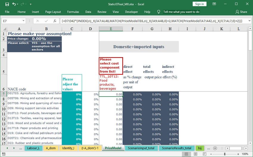
ABSTRACT

In the last two decades, the application of Input-output (IO) models has increased due to
general availability of extensive structural data sets, esp. IO tables, and the increase in
computing power. Today, a broad range of different IO models and applications exists –
from simple, static to comprehensive, dynamic IO models.
Simple static IO models are used for comparative-static scenario analysis. With the help of
IO quantity models, statements can be made about direct and indirect effects based on
exogenous changes in demand. However, these are to be interpreted against the back-
ground of their limitations and assumptions such as the time-independency and the non-
consideration of feedbacks such as income and price effects. In contrast to the static IO
quantity model, the static IO price model is able to capture the effects of input factors such
as wages on sectoral production prices. Hereby it is assumed that cost changes are passed
on completely and directly. No volume adjustments are made by substitution processes of
the customer industries. Both model types can be easily implemented in Microsoft (MS)
Excel which provides the necessary functionalities (e. g. matrix algebra functions) without
any need for programming tasks. Another advantage is that most IO tables are distributed
in MS Excel file formats, e. g. xlsx.
More complex dynamic IO models largely resolve the limitations and inherent assumptions
of static IO models. Time is considered explicitly as well as quantity and price reactions are
modelled endogenously in a holistic approach and feedback effects are captured. Thus,
such models are not only suitable for scenario analysis but also for forecasting. Due to the
increased complexity of dynamic IO models, their implementation usually requires exten-
sive programming tasks. Commonly used programming environments are EViews, R or
MATLAB.
In this paper, we will show that MS Excel is suitable for the implementation for both static
and dynamic IO models. First, we will present a template for a static IO quantity and price
model with free available data for Mexico. Second, a template named DIOM-X is discussed
which contains all the necessary tools to build a dynamic IO model in MS Excel and its
programming language Visual Basic for Application (VBA). The template contains all the
necessary tools to perform both scenario analysis and forecasting (data management, re-
gression analysis, model execution engine, presentation of model results). This approach
greatly simplifies the task of building a dynamic IO model: Existing knowledge in MS Excel
can be used, most computers are already equipped with the software and thus don’t any
additional software licenses and setup and models may be easily shared or distributed by
just transferring one file.

                                                                                           4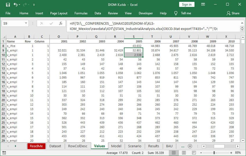
1 INTRODUCTION

In the last two decades, the application of Input-output (IO) models has increased especially
due to the increase in computing power and the general availability of extensive structural
data sets, esp. IO tables.
Common tasks such as inverting a matrix or solving equation systems which in the past
could only be accomplished on expensive workstations or mainframe computers can now
be calculated in seconds or a few minutes by cheap desktop or notebook computers. Model
builders can now choose from a wide range of programming languages (e. g. Python1) and
integrated application frameworks (e. g. GAMS, Eviews).
Today’s internet technology greatly simplifies the task of collecting the necessary infor-
mation to build an IO model. In the past, the data had to be extracted either from books or
later CD-ROMs. A lot of time-consuming, tedious work was necessary to be able to build
the IO database. In recent years, the internet technology greatly simplified the process of
data publishing: The number of data sources increased dramatically while the up-date-cy-
cles became much shorter (e. g. the online version of the Eurostat database (https://ec.eu-
ropa.eu/eurostat/data/database) is updated daily). Furthermore, the number of data formats
has been reduced over time which makes data processing less time-consuming. For desk-
top data processing, most data providers offer either MS Excel, CSV (comma-separated
values) or XML (extended markup language) files. In order to be able to use the data in an
IO model, it still has to be processed. Most model building tools require the data to be ar-
ranged in a certain layout (e. g. values in columns). Even more importantly, variable names
(and types) have to be assigned to the data before it can be accessed in the model.
Even with these powerful technologies at hand, the task of building IO models is still a
challenge. A potential model builder has not only to get acquainted to IO theory but must
have profound knowledge in information technologies (i. e. data processing, programming,
spread-sheet programs).
IO models greatly differ in size and possible applications. Simple static IO models are used
for comparative-static impact (scenario) analysis. With the help of IO quantity models, state-
ments can be made about direct and indirect effects based on exogenous changes in de-
mand. However, these are to be interpreted against the background of their limitations and
assumptions such as the time-independency and the non-consideration of feedbacks such
as income and price effects. In contrast to the static IO quantity model, the static IO price
model is able to capture the effects of input factors such as wages on sectoral production
prices. Hereby it is assumed that cost changes are passed on completely and directly. No
volume adjustments are made by substitution processes of the customer industries. Both
model types can be easily implemented without any programming tasks. The necessary
functionality (i. e. basic algebra, data file format support) is already provided by spread-
sheet programs such as MS Excel of OpenOffice. In chapter 2, the implementation of such
a model in MS Excel is discussed for the Mexican economy but could also be used for other
countries.

1   Nazara et al. 2003 used Python for IO analysis.

                                                                                           5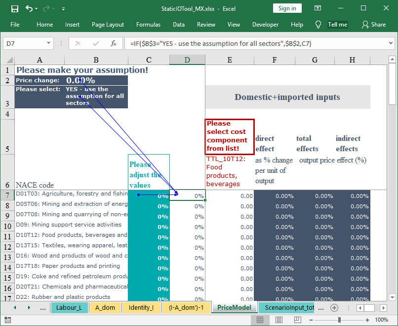
More complex dynamic IO models largely resolve the limitations and inherent assumptions
of static IO models. Time is considered explicitly; quantity and price reactions are modelled
endogenously in a holistic approach and feedback effects are captured. Thus, such models
are not only suitable for scenario analysis but also for forecasting. Due to the increased
complexity of dynamic IO models, their implementation usually requires extensive program-
ming tasks. Potential model builders first have to decide on their development environment.
They can either build their own development environment by selecting one out of the hun-
dreds of common programming languages (which all have specific strengths and weak-
nesses) and collecting or implementing programming libraries which carry out specific tasks
(e. g. handling of times-series data, matrix algebra). Another option is to get acquainted to
a (costly) all-in-one application framework such as GAMS or Eviews. With each of these
options, potential model builders will be facing a steep learning curve before they can fully
exploit the power of these systems.
Another option to build a dynamic IO model is to use MS Excel not only for data preparation
but to build a fully-fledged model in the integrated programming language VBA (Visual Basic
for Applications). This approach offers some important advantages:
      1. MS Excel is widely used for data processing and evaluation. Thus, most poten-
         tial model builders are already familiar with at least the basic functionality.
      2. Most computers which are used in an professional environment are equipped
         with the MS Office program suite and are therefore prepared for model develop-
         ment.
      3. A model which is fully built in MS Excel can be easily shared or distributed to
         other users.
      4. There is no need for buying other (expensive) model building tools.
      5. By reusing existing knowledge in operating MS Excel, the time needed to build
         a model is greatly reduced which is important for projects with tight time and/or
         budget restrictions.
In chapter 3, a template for a dynamic IO model and its technical implementation into MS
Excel is discussed. Chapter 4 concludes and gives some ideas about further development.

2 STATIC INPUT-OUTPUT MODELS

2.1 OVERVIEW

Standard IO models are able to reveal how different sectors of an economy are intercon-
nected and how changes in one sector affect all other sectors. Their application relies on
an IO table providing a comprehensive picture of the supply of goods and services by do-
mestic production and imports, its composition by intermediate consumption and value
added as well as the use of goods and services for intermediate and for final consumption,
for gross capital formation and exports.

                                                                                           6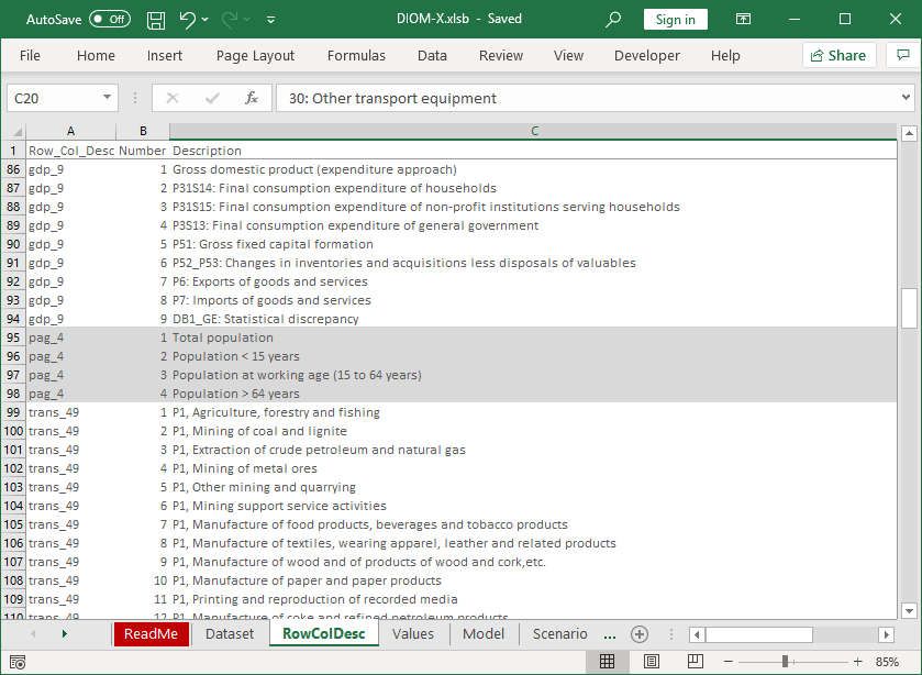
Besides the use of the IO data for descriptive analyses of economic interrelations, this table
also provides the empirical fundament for a wide scale of impact analyses of e. g. govern-
mental programs in different fields on domestic production, income and employment. The
basis of this kind of analysis is the Leontief equation. Equation (1) shows the reduced form
of this equation whereby production x is determined by final demand y and the Leontief
inverse ( − ) which incorporates the input coefficient matrix A and the identity matrix I
(Eurostat 2008, Leontief 1986).
    (1)       =( −       )       ∙
All components of this equations can be derived from an IO table. The resulting set of linear
equations (Leontief quantity model or demand pull model) can be used to answer questions
such as ‘what happens to the output if final demand due to export promotion or investment
changes?’ The results show the impacts on the economy to satisfy an additional (final) de-
mand and give insights into the industry-wide effects (direct and indirect effects).
If the number of employees by industry is also known, the implications for the labour market
can be derived in addition to the output effects. Based on equation (1), production-induced
employment effects e can be computed by multiplying with employment coefficients b
(equation (2)).
    (2)       = ( −          )       ∙
Another application of the IO table is the Leontief price model (or cost push model, (Miller,
Blair 2009, Eurostat 2008, Oosterhaven 1996). It rests on equation (3) where p’t is the out-
put price, ( − ′ ) is the transposed Leontief inverse, Q is the diagonal matrix with unit
factor price for primary inputs and v are the input coefficients for primary inputs.
    (3)     ′ =( − ′ )
It can be used to evaluate the impacts of changes in cost factors such as wages, fuel or
import prices on output prices by industries.

2.2 IMPLEMENTATION INTO MS EXCEL

The practical implementation of the Leontief demand-pull and cost-push models in Excel is
straightforward. In the following subsections the steps to be taken are described in short for
both models.
A prerequisite for building a Leontief model is an IO table. For our illustration purposes, we
use an IO table for Mexico downloadable from OECD website (https://stats.oecd.org) which
includes an IO table for imports, domestic production as well as the total IO table in the ISIC
Rev. 4 classification. Employment data are available at STAN Database for Structural Anal-
ysis (ISIC Rev. 4, SNA08). These data are the basis for the development of the static open
impact analysis tools.
The original data are included in the Excel workbook StaticIOTool.xlsx2 in different work-
sheets as listed below:

2   This tool will be made available on request. Please contact the authors.

                                                                                            7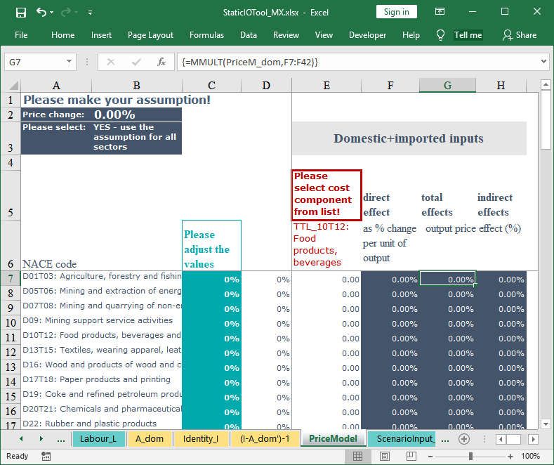
•      zij_Xj includes the symmetric IO table in million USD
•      zij_im includes import matrix in million USD
•      zij_dom includes domestic production matrix in million USD
•      Labour includes the employment data in 1,000 persons
All worksheets in the workbook StaticIOTool.xlsx with original data are coloured in white.
The other worksheets contain the calculation steps to derive the linear equation set for the
Leontief quantity model and price model. The scenario input form and results sheet for the
price model is coloured in dark blue, for the quantity model in turquoise (Figure 1).

Figure 1:        Static Impact Analysis Tool

2.2.1 LEONTIEF QUANTITY MODEL
The following steps have to be taken to build the open Leontief quantity model:
       (1)    Calculation of input coefficients
       (2)    Calculation of Leontief-Inverse
       (3)    Calculation of labour coefficients
       (4)    Prepare scenario input form
       (5)    Prepare scenario result sheet
The following explanations only refer to the implementation in MS Excel and do not explain
IO theory and the derivation of the Leontief equations (for this please refer e. g. to Leontief
1986, Miller, Blair 2009).
Excel offers helpful functions like array formulas, which make cell by cell links superfluous.
Furthermore, the name manager offers possibilities to define names for ranges, e. g. inter-
mediate demand matrix that can be used for further calculations. Named ranges are much

                                                                                            8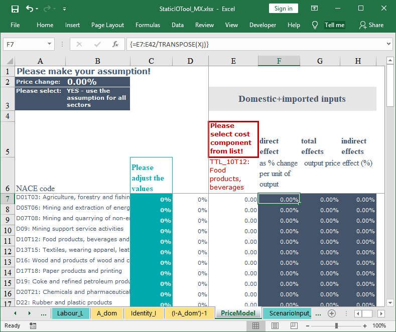
easier to understand and maintain as Excel calculations can often be written just like the
formulas in a text book.
In the first step the input coefficients for domestic intermediates Aij_dom need to be calcu-
lated by dividing domestic intermediate inputs zij_dom by total output xj. Instead of applying
the division in each cells of the A-matrix, the use of the name manager and array formulas
are suggested.
To define a name, go to the Excel menu bar, select Formulas tab and click Define Name.
A new dialog window shows up. In the field Name enter a name, e. g. zij_dom for the vari-
able. Then select the field Refers to and mark the associated cells in sheet zij_dom. Finally,
click the OK button (Figure 2). After finishing these steps, the name should appear in the
name manager.

Figure 2:        MS Excel: name manager

After defining the names for the variables used in the formula, the domestic input coeffi-
cients are calculated using an array formula. For this, select all cells where the formula
should be applied to. In the formula bar the equation – using the defined names – is inserted.
Then, press Ctrl + Shift + Enter. The formula is enclosed by curly brackets {} and for the
selected dimension the values are calculated according to the formula (Figure 3).

Figure 3:        Leontief quantity model: calculating input coefficients for domestic interme-
                 diates by using defined names and array formula

In the next step, the Leontief-Inverse is calculated for which an identity matrix I needs to be
created. MS Excel 2013 and 2016 provide the MUNIT()-function that returns an identity

                                                                                            9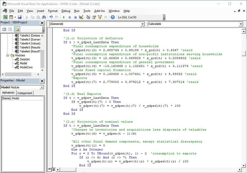
matrix for the specified dimension. First, select the dimension of the identity matrix. Then,
type the formula =MUNIT (dimension, e. g. 36) as an array formula (Ctrl + Shift + Enter). A
36x36 matrix with the value one along the diagonal will appear. For matrix inversion, MS
Excel provides the MINVERSE() function that can be used for calculation of the Leontief
equation.
After the derivation of the Leontief equation, the scenario input und result sheet needs to
be prepared. Here, the quantified inputs of a scenario (expressed as a change of final de-
mand) will be introduced (Figure 4).

Figure 4:        Leontief quantity model: Scenario input sheet

The scenario input(s) have to be linked to the input and employment coefficients. To calcu-
late the direct, indirect and total input coefficients for production, the inputs from the sce-
nario input sheet are multiplied by the respective coefficient matrix (Figure 5).

Figure 5:        Leontief quantity model: scenario results sheet

The Excel function for performing matrix multiplication is MMULT(). The employment effects
are calculated by linking the production effects (given in the results sheet) and the labour
coefficients.

                                                                                            10
2.2.2 LEONTIEF PRICE MODEL
The development of the Leontief price model comprises the following steps:
(1) Calculate input coefficients for domestic intermediates
(2) Calculate price equation = ( − )
(3) Prepare price model sheet
The first two steps can be done easily by using the Excel matrix functions MINVERSE() and
TRANSPOSE(). The worksheet “price model” includes the input form for scenario assump-
tions as well as the results.
Figure 6: Leontief price model: input and result sheet (I)
There are three scenario input cells: In cell B2 the price change assumption is given (Figure
6). In the cell B3 it is specified if the price change assumption is applied for all 36 industries
or only for selected industries. In the cell E6 the cost component to which the price change
should be applied is given.
In cell B3 a list with two entries is created: Either the price assumption is applied to all
industries or only for selected industries. The list to be created includes the following two
entries: YES - use the assumption for all sectors, NO - adjust values for each sector indi-
vidually. The text is given in the field Source (Figure 7).
To create a list, first go to the excel menu bar, select data and click data validation. A new
dialog window shows up (Figure 7). In the tab ‘Settings’ select in the field Allow: ‘List’. Then,
in die field Source enter a text or link to the source. Finally, click the OK button.
11Figure 7: Creating a list in MS Excel
In cell F6 another list is created based on the cost components that are given in the domes-
tic flow matrix (sheet zij_dom). Instead of typing each list entry by hand, references to range
C9:C48 in sheet zij_dom are used.
The scenario input for all industries is given in cell B2. If the values should be adjusted only
for selected industries they have to be given in column C for the suitable industries (rows).
Depending on the YES / NO selection in cell C3 either the value that is given in cell B2 or
the values given in column D should be used as an input for the IO price model. The Excel
IF()-Function is applied in column D to select the appropriate values (Figure 8).
In column E the value of each industry given in row 7 to 42 of a selected cost component in
cell E6 is shown. As an example, if the industry ‘Food products; beverages’ needs input
from the industry ‘Agriculture, forestry and fishing’ then the value given in the domestic flow
matrix is linked to cell E11 and multiplied by the assumed price change.
12Figure 8: Leontief price model: input and result sheets (II)
Therefore, depending on the selected list entry and the price change assumption the values
in range E7:E42 change automatically. The following array formula combining the Excel
INDEX() and MATCH() functions is used:
13Figure 9: Leontief price model: input and result sheets (III)
To calculate the direct output price effect by industry as percentage change per unit of
output (column F), entries in column E are divided by the production by industries Xj (Figure
10).
Figure 10: Leontief price model: input and result sheets (IV)
The total price effect (column G) is calculated as an array formula by multiplying the price
equation ( = ( − ) ) and the direct effect given in column F (Figure 11).
14Figure 11: Leontief price model: input and result sheets (V)
The indirect price effect (column H) is calculated by subtracting the direct effect (column F)
from the total effect (column G).
2.2.3 SCENARIO ANALYSIS
Once the impact analysis tools are implemented, they can be used for impact analysis which
is a technique that analyses the possible consequences (or impacts) of a measure of a
future event that is specified in a scenario (e. g. export promotion programs, wage in-
crease). The analysis is comparative-static meaning that a situation before and after an
exogenous change is compared but the adjustment process is neglected.
An impact analysis starts with the (1) choice of a policy measure or initial change that should
be analysed (scenario design). Then, the appropriate tool (Leontief quantity or Leontief
price model) has to be selected. The Leontief quantity model is applied if the direct and
indirect impacts of final demand e. g. due to export promotion or investment changes should
be evaluated. The Leontief price model is used to evaluate the impacts of changes in cost
factors such as wages or fuel prices on output prices by industries.
(2) The policy measure needs to be translated into an impulse – either a change of final
demand (Leontief quantity model) or changes in e. g. wages or fuel prices. Furthermore,
one or more of the 36 industries that are affected have to be selected.
Afterwards (3), the impacts on production and employment (Leontief quantity model) or out-
put price effects (Leontief price model) are evaluated. In the Excel tools, all results will be
updated immediately and automatically.
152.3 CONCLUSIONS
Both model types – the open Leontief quantity model and Leontief price model – can be
applied for specific purposes but have their advantages and limitations (see for example,
ILO 2017, Großmann et al. 2016, Oosterhaven 1996, Holub, Schnabl 1994).
The advantage of static IO models is that the industry structure and relations are clearly
described and transparent, so that the status quo of the value chains, supplier and customer
relationships can be analysed comprehensively. Key industries and industries which are
vulnerable to exogenous price and volume effects can be identified by applying a compar-
ative-static analysis which show direct and indirect impacts.
Limitations of IO models consist in the assumption that the input structure is fixed (so-called
limitational production function) and there are constant returns to scale. There is no substi-
tution of inputs across industries. Future technological changes and innovations are ne-
glected and therefore static IO models might be useful in the short run but cannot be used
for analysing structural changes. In the Leontief price model, this restriction (constant input
coefficients) implies that changes in costs are passed on completely to downstream indus-
tries and they cannot substitute the more expensive input factors by cheaper products. Cus-
tomers are assumed to be price takers, so that the demand will not change.
Capacity constraints are not considered in the Leontief quantity model. If capacity utilization
is high, producers may not be able to satisfy the additional demand in full without investing
in e. g. new machinery. Additional demand might also be satisfied with imports. Thus, re-
sulting impacts of a scenario may be overestimated. Furthermore, prices are assumed to
be fixed and do not respond to demand shocks. Another aspect – not part of a static open
IO analysis – is that the income effect occurring with a higher employment level causes an
additional higher demand for consumer goods.
There are many applications of the static IO models. Well-known are for example, IMPLAN
(www.implan.com), REMI and RIMS II (BEA (n.d.)) which have some extensions to the very
basic static IO model described in this chapter but are still not dynamic IO models which
are described in the next chapter.
3 DYNAMIC INPUT-OUTPUT MODEL (DIOM-X)
3.1 OVERVIEW
In contrast to static IO models where the structure of the economy is assumed to be con-
stant, dynamic IO models3 consider developments over time. The dynamic IO model pre-
sented in this chapter is based on the INFORUM approach (Almon 1991, 2014).
As with static IO models, the IO relationships are the focus of the analysis. The models are
typically demand-side driven. However, the demand is determined endogenously and not
3 For examples of dynamic IO models please refer to e. g. Thijs 2017, Eurostat 2008, pp. 527, West 1995,
Kratena et al. 2013
16given exogenously. The economic cycle is completely represented by the national ac-
counts, so that for the main economic sectors a. o. private households, companies and
government, production, income generation and redistribution to consumption can be
shown. An important variable in the national accounts (SNAB) is disposable income, which
is influenced by both the current labour market situation and the redistributive activities of
the government through taxes and subsidies. In addition to other variables such as selling
prices, disposable income, it is an important determinant of private consumer demand.
The link between demand and supply is given by the Leontief production function. Further-
more, the IO table shows the cost structure for each industry given by demand for interme-
diate goods and used primary inputs such as compensation for employees, depreciation,
net taxes on production. Prices are derived by using a unit cost approach considering the
single cost components. Production prices plus net taxes on goods determine purchasers
prices. The latter determine, in addition to disposable income, the demand of private house-
holds.
In contrast to simple static IO models, the volume and price reactions in this macro-econo-
metric IO model are empirically based and take the passing on of costs into account and
thus include the competitive situation on the different product markets and the labour mar-
ket.
Supplementary data are population by age groups, employment and wages by industries.
Population at working age determines the work force. Labour demand is determined at in-
dustry level and related to real production and wages by industries. Increasing real wages
tend to lower employment while a higher production level will increase employment. The
macroeconomic wage rate is determined by using a Phillips curve approach.
Exogenous
System of National Accounts Estimated
By definition
Unit Costs
IO framework
Intermediate Intermediate
Final Demand
inputs Demand
Labour Costs
Depreciation Value Added
Production
Other Net Taxes
of Production
Prices
Labour market
(Employment, Population
Wages)
Figure 12: Simplified illustration of a dynamic IO model
Source: own illustration
The model contexts shown in Figure 12 are captured both via identities (e. g. in the IO
context) and behavioural equations that are empirically validated. Using econometric
17methods allows for imperfect markets and bounded rationality (Meyer, Ahlert 2016). How-
ever, the specification of the model is not finished with the estimation of single equations.
The complete, non-linear, interdependent model equation system is solved iteratively for
each year using the Gauss-Seidel algorithm. The iteration process is ended once a given
criterion is fulfilled. This criterion has to be an endogenously calculated model variable, e. g.
output. As long as the model has not converged, all model equations are recalculated for
the current year. Afterwards, all equations are solved for the next years within a given time
span. The model template contains the necessary code for the iteration algorithm. A model
builder might redefine the criterion.
Exogenous impulses for the model are, for example, population development and exports,
which trigger adjustment reactions in the highly interdependent, non-linear model. The mod-
elling approach which covers not only quantity effects but also income and price effects,
provides further multipliers that determine the dynamics of the system:
Leontief multiplier: shows the direct and indirect effects of demand changes (e. g.
consumption, investments) on production;
Employment and income multiplier: Increased production leads to more jobs and
thus higher incomes resulting in higher demand (induced effect);
Investment accelerator: Indicates the necessary investments to maintain the capi-
tal stock needed for production based on the demand for goods.
Dynamic IO models exist in different forms and degrees of complexity (see e. g. Eurostat
2008, pp. 527, Stocker et al. 2011, Lehr et al. 2016, Ahlert et al. 2009, Großmann, Lutz
2017, Großmann, Hohmann 2016, Cambridge Econometrics 2014, Lewney et al. 2019).
For example, IO models can be modelled bottom-up and top-down: bottom-up indicates
that each industry respectively product group is modelled individually and macroeconomic
variables are calculated through explicit aggregation. Top-down means that first, the final
demand components are determined at the macro level and then are disaggregated ac-
cordingly e. g. by using the industry or product shares of the respective variable.
In the following, a template for a simplified dynamic IO model is developed and implemented
in MS Excel VBA.
3.2 TECHNICAL FOUNDATION
3.2.1 ESSENTIAL PROGRAMMING LANGUAGE FEATURES
Today, hundreds of programming languages exist and each of them has been developed
to overcome some problems or to improve certain features of other languages. In principal,
almost any of these programming languages may be used to build an dynamic IO model as
long as at least the following features are provided.
A dynamic IO model is processing data over time, thus the language has to support multi-
dimensional data structures. These are called array in most programming languages. Some
languages such as Python do not have a built-in array type. This is not a problem as long
as programming libraries are available which offer array-like data structures (for Python, a
well-known library for numeric data processing is named “Numpy” (www.numpy.org). In
some languages, array-indexing is zero-based (e. g. C, C++) whereas in other languages
18the first element in an array has the index one. The latter is preferable since most of the
published data and sector classifications use one-based indices.
Array-like data structures are not only necessary to process data over time but also to han-
dle data which contains more than one value per year (e. g. sectoral data, IO matrices). For
most use-cases, three-dimensional structures are sufficient, i. e. to store a sequence of IO
matrices. The speed of indexing into arrays greatly differs between programming languages
and is quite important because a comprehensive dynamic IO model contains a considerable
amount of these statements. The following table shows the processing time for setting each
element in a 10,000x10,000 double-precision floating point array in some popular program-
ming languages4. The most simple built-in array implementation in each of the languages
was used to receive comparable results.
Interpreted languages are the slowest because instructions are processed one-by-one with-
out much room for optimizations. Compiled code performs fastest because the program as
a whole is translated into machine-executable form and usually highly optimized. JIT (Just
In Time)-compiled code is often almost as fast as compiled code by translating the program
into an intermediate, processor-independent code which is then translated into processor-
dependent code at run-time. The table shows that Excel`s built-in VBA language – although
it is an interpreted language – performs more than acceptable in comparison to other lan-
guages.
Table 1: Processing time for array element processing (10k x 10k elements) in se-
lected programming languages
Source: Own calculations
Language Time (s) First Index Language type
Eviews 9 93 1 Interpreter
Octave 5.1 435 1 Interpreter
R 3.6.1 2628 0 Interpreter
Python 3.6 54 0 Interpreter
Julia 1.0 4.5 1 Interpreter
VBA 2016 5 1 Interpreter
VBScript 5.812 19 0 Interpreter
C# Interactive 3.1 0.5 0 JIT Compiler
Java JDK 1.8 0.2 0 JIT Compiler
C# .NET 4.7 0.6 0 JIT Compiler
MinGW C++ 7.3 0.3 0 Compiler
Additional essential features which are provided by almost every programming language
are
loops to be able to iterate over time as well as to address elements in a multidi-
mensional data structure
4 The size was chosen to simulate a comprehensive model with a lot of indexing statements The calculation
was done using an Intel i7-8600k processor with 32GB RAM. The code is available on request.
19 conditional statements to differentiate cases in order to be able to execute different
branches of code
sub-programs (functions, procedures) to create reusable subroutines
modules to divide a program into logical parts
A few programming languages support matrix and vector algebra (e. g. Matlab, Octave)
which makes equation statements much more readable. For languages lacking this feature
– VBA belongs to this group –, matrix and vector algebra must be implemented by using
“functions”. The missing functionality is often available in the form of programming libraries
which can be downloaded or purchased as add-ons. The model template contains a few
additional algebraic functions in order to perform the necessary calculations in the model.
In order to track down errors, a debugger is extremely useful: Code may be halted at any
statement (often called break) as well as data may be evaluated at run-time when the pro-
gram has been interrupted by a “break” instruction. Some debuggers even allow for evalu-
ating expressions while the program is in interrupted state. MS Excel has a built-in debug-
ger which supports these features.
3.2.2 EXCEL VBA LANGUAGE AND PROGRAMMING ENVIRONMENT
In VBA, (multi-dimensional) arrays may be declared by using the Dim or Redim statements
with the proper bounds given for each dimension 5 . VBA does not directly support
matrix/vector algebra but provides functions for some essential tasks such as matrix
inversion (MINVERSE()) and matrix multiplication (MMULT()) which is needed e. g. for the
calculation of the Leontief-Inverse. The model template contains additional functions for
those that are missing in VBA, e. g. vector addition. In this regard, Excel is not as powerful
as other software solutions which might be used for model building.
The variables are empty at program startup and must be filled by reading the data from the
worksheets. The model template which is described in section 3.4.4 comes with a simple
dataset manager that automatically translates the list of model variables into VBA
declarations.
After the model has finished the calculations, the data is transferred back into dataset
worksheets. Performing all calculations on arrays is magnitudes faster than reading/writing
worksheet cells.
VBA provides the for loop statement for a fixed and the while loop statement for a varying
number of iterations. The select case statement is useful if a certain statement out of a
group of statements shall be executed. The if statement is used when code must be
executed with respect to the result of an evaluated expression.
Subroutines may be implemented by using a sub … end sub block. If a subroutine has a
return value, the statements have to be embraced by a function … end function block.
Excel stores all model code along with the data in a *.XLSM (XLS with macros) file or *.XLSB
(binary) file. The XLSB format usually offers better compression and loading/saving times.
Small to medium size models with some hundred variables may be conveniently stored with
5 Multi-dimensional arrays are easier to set up but make some algebraic calculations more complicated.
20all the code in just one file. The setup and distribution of such a model can therefore be
accomplished by just distributing one file to the recipient. With bigger models, it might be
more convenient to use separate files, e. g. by separating historical and forecasted data.
By default, the VBA programming environment (Figure 13) is not visible with a default
installation of MS Excel or Office, most likely because only the minority of users is using the
programming features. The environment can be activated by pressing Alt+F11 or by
activating the Developer menu entries under Options, Customize Ribbon.
The project pane gives access to the VBA code which may either be attached to worksheets
or be stored in user-created modules. The text editor with syntax highlighting is used to edit
the code. The evaluator is helpful for inspecting variables at runtime and for evaluating
expressions. By clicking the grey vertical bar next to a certain line in the text editor, a
breakpoint may be set in order to suspend the program for error checking, expression
evaluation, etc.
Figure 13: MS Excel: VBA programming environment
With the combination of the data stored in worksheets and the VBA programming
environment which allows for editing and storing the model code along with the data, a
potential model builder has all the necessary tools at hand to start building dynamic IO
models.
3.3 STEPS IN MODEL BUILDING
The main steps of building a dynamic IO model are:
1. Database management
2. Regression analysis
3. Core model building
4. Forecasting and scenario analysis
21It has to be pointed out that model building is not a sequential process. The model building
steps may have to be repeated under certain conditions, e. g. availability of updated or
additional data, errors that has been tracked down to previous model building steps or the
need for more detailed specifications.
1. Database management
The foundation of every quantitative model is data collected from different sources, i. e.
official sources (national and international statistical offices, e. g. Eurostat, OECD.stat). The
selection and quantity of data depends on the aim of the modelling exercise.
Data from different sources usually comes in different file formats (e. g. CSV, MS Excel).
Even if the file format is the same as with Excel files, data is often organized differently:
Time series data may be stored in rows or columns or spread over different sheets. Matrix
data may be stored in worksheets or different files (workbooks).
The first important step in building the historical database is to harmonize the data structure
by creating a unified dataset where each data item shares the same layout.
One important property missing from original data is the naming of each variable which is
needed to access its values from within the model. It is advisable to develop some sort of
naming convention which is shared between model builders in order to be able to identify
and address each variable in the data set. Additional meta information such as unit, dimen-
sion and source should be collected accordingly to further describe the content of the da-
taset (“meta information”). This information is often useful to avoid errors in certain compu-
tational statements such as unit conversions. The model template contains worksheets for
both the harmonized dataset and the list of variables with placeholders to fill in this important
information.
2. Regression analysis
The availability of historical data is the most important prerequisite for regression analysis
which is carried out by econometric models to estimate model parameters for behavioural
equations. Instead of using elasticities from the literature, relationships of variables known
from e. g. economic theory are econometrically tested against historical data. Regression
results (parameters/coefficients) show the direction and magnitude of the relation between
the dependent (or left hand side (LHS) variable) and independent variable(s) (or right hand
side (RHS) variable(s)). In contrast, variables that are given by definition have a fixed rela-
tion to each other.
For example, theory tells that there is a relation between consumption and disposable in-
come. Relative prices and population can play an additional role. Finding the appropriate
specification heavily depends on data availability and quality. Furthermore, even with the
same specification of the regression equation, the estimated parameters may differ for dif-
ferent countries. That is not really astonishing because people in different countries show
different consumption behaviours. Even within one country their behaviour may change
over time.
In DIOM-X, regression analysis can be carried out using built-in MS Excel functions such
as RGP(). Other econometric software such as EViews or R can be used as well. Like with
most other model building environments, the data need to be manually transferred to
22another statistical program and after estimation the parameters must be manually imple-
mented in the model code.
3. Core model building
The main task of this model building step is to create the model structure by putting the set
of equations together. Most equations – both regressions and definitions – are not inde-
pendent but interrelated. LHS variables of one statement occur as RHS variables in another
equation. Therefore, the model builder has to carefully define the sequence in which the
equations have to be calculated. The model building itself follows the IO approach (Leontief
1986, Miller, Blair 2009). In section 3.4.4, the model template used as an example for a
dynamic IO model is introduced.
Furthermore, the model should be divided into logical blocks which then can be imple-
mented (often independently) in the programming language instead of creating a monolithic
program structure. The template is organized as a set of modules which interact with each
other. It contains modules for the model-independent calculation engine, generated parts
such as the variable declarations and model codes.
The template’s calculation engine keeps the values constant for those variables for which
no computation statements (i.e. regression or definition) have been implemented. This ap-
proach makes sure that the values of a such variables cannot drop to zero or are not defined
in the forecasting part.
MS Excel’s VBA programming language in combination with the pre-structured model tem-
plate greatly simplifies the task of implementing the model. For example, the calculation of
GDP can be written as
v_vacp(t) = v_gosmi(t) + v_coe(t) + v_otlsp(t) with
v_vacp (t): Value added at current prices
v_gosmi (t): Gross operating surplus and mixed income
v_coe (t): Compensation of employees
v_otlsp (t): Other taxes less subsidies on production
For more please refer to section 3.4.
4. Forecasting and scenario analysis
The DIOM-X model template implements a dynamic IO model, thus all model equations –
definitions and behavioural equations – are solved year by year during the simulation pe-
riod. A forecast usually covers a time span of 10 to 30 years. Due to many feedback linkages
the model has no explicit solution and solves all model equations iteratively. The iteration
process is ended once a given criterion is fulfilled: For a central model variable, the deviation
in percent between two consecutive iterations has to be smaller than a given value (e. g.
an output deviation of less than 0.1 % for each industry).
The inherent uncertainty of the future makes it impossible to forecast one 'real' prospective
development. The outcome of the most basic forecast is based on the assumption that past
behaviour is also effective in the future (business as usual scenario, BAU). Scenario anal-
ysis is a method to handle uncertainty and to carry out 'what if'-analysis especially to ana-
lyse the impacts of policy measures before implementation. A scenario consists of a set of
23consistent assumptions which are fed into the model. With DIOM-X, this task becomes ex-
tremely easy by typing the desired variable names and values into the Scenario worksheet
(see section 3.4.4). The alternative scenario is then calculated within a few seconds. Com-
paring two scenarios reveals differences at a specific point in time and over time (Figure
14) that can be interpreted as reactions to the impulses induced by the initial changes.
Figure 14: Comparing scenarios
From a technical point of view, scenarios are adjustments of the value of one model variable
or a set of model variables.
A DIOM-X model not only stores the historical data but also the forecasted data which
makes it straightforward to visualize the data appropriately (e. g. by creating a management
summary graphs and tables for the most important variables).
3.4 IMPLEMENTATION INTO MS EXCEL
The following sections describe a simple, yet useful template for building a dynamic IO
model in MS Excel step-by-step.
3.4.1 DATA MANAGEMENT
In order to retain the usability of an IO model, it often needs to be extended, revised and
updated. Its foundation is the historical data set and the quality of the latter has a great
impact on the model results. Thus, the data management plays an important role in the life
cycle of a model. The time and effort that has to be spend on building the historical database
for an elaborated IO model is often underestimated:
Most data providers offer data in Excel format but the layout of such files is not standardized
so that often the data needs to be converted into a format the model is able to handle.
Data providers from time to time change the layout of their data files which requires that
the data processing routines need to be revised.
In order to be able to perform calculations inside the model, each time series has to be
given a name. From a model’s perspective, the variables with their associated data are
24sufficient to carry out the calculations. From a modeller’s perspective, additional information
(“meta data”) is needed to keep the model complexity under control, e. g. a description for
each variable and its dimensions, units, data source, last revision, etc.
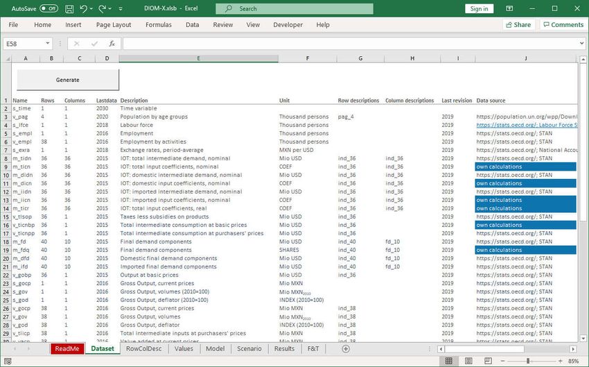
Figure 15: Worksheets Dataset and RowColDesc
While for the model execution only the number of rows and columns is needed, the model
builder needs to lookup the description of the elements which are given in worksheet
25RowColDesc (Figure 15 above). The entries in column G and H in Figure 15 (top figure)
refer to the associate description in worksheet RowColDesc.
The DIOM-X framework provides the Dataset worksheet in which the data contents of the
model need to be defined. Each row in the worksheet defines one variable with its basic
information such as variable name, last year of available data (lastdata) and the additional
meta data such as data source (Figure 15).
By pressing the Generate button, the framework automatically translates the full data set
(the list of variable definitions) into appropriate VBA variable declaration code.
A model builder should also keep in mind that with a rich dataset, defining variables names
becomes a challenge on its own: Very short abbreviations are hard to remember whereas
longer, expressive names take much more time to type when it comes to coding. It is rec-
ommended to establish some sort of convention which defines a set of rules for naming the
variables of the dataset. The convention used for the DIOM-X model template reads as
follows:
Each variable name starts with a letter which describes the variable type followed by an
underscore: s_ means (time) series, v_ describes a vector and m_ names a matrix.
For the name part, the first letter of each noun of the variable description is used, e. g. fd
means final demand.
The variable names are composed of lower case letters only.
In order to assign the historical values to the variables in the dataset, the template contains
the Values worksheet (Figure 16):
Figure 16: Values worksheet with data
For each variable (and in case of vectors and matrices for each element), the model builder
needs to the variable name, row and column numbers and values for each year. The model
26framework reads in this worksheet prior to execution. The worksheet can be created in
different ways, depending on the structure and size of the dataset as well as the skills of
the model builder:
Data can be manually copied and pasted from the original data files (not recommended)
Data may be linked to the original data sources
The worksheet could be the output of a data processing program
A mix of the aforementioned options
After successful model execution, the framework automatically copies the full historical da-
taset as defined in this worksheet as well as the forecasted data to the Results worksheet
for further processing and evaluation.
3.4.2 REGRESSION ANALYSIS
If the parameters are not taken from the literature, they must be determined on the basis of
the country-specific data set. Excel provides the RGP() function which does linear regres-
sion using the least squares method. Other econometric software such as EViews or R –
which provide more statistical techniques – can also be used. The user needs to transfer
the dataset from the worksheet Values to the program of his choice to perform the estima-
tions.
The authors use the econometric regression program G76. In the model template (see Fig-
ure 23), the variables are marked with dashed lines, whose parameters are explained econ-
ometrically. Among them are macro / time series (e. g. labour force s_lfce) as well as vector
variables (e. g. GDP components v_gdpev).
The following steps describe the procedure of getting macro and vector regressions into the
model:
The parameters for the labour force equation are derived by using the OLS technique. At
the left hand side of the equation, the variable to be explained is labour force s_lfce(t) and
on the right hand side is the explanatory variable v_pag(t)(3) which is population at working
age (see red arrow in Figure 17). Based on the Mexican dataset, the estimation includes
historical data from 2005 to 2018.
The parameters (Reg-Coef) of the regression equation are shown in Figure 17 (red box) as
well. The equation and the parameters must be transferred manually into the VBA code at
an appropriate position which is determined by the model logic created by the model builder
(Figure 18).
6 http://www.inforum.umd.edu/software/g7.html
27Figure 17: Regression example I
The latter part of the equation is the error term which corrects the estimated value in the
last year for which historical data is available. This term ensures a smooth development
between the historical and projected data (red circle and graph in Figure 17).
Figure 18: Implementing regressions into the VBA code I
A log-log estimation is done to derive price-adjusted GDP components v_gdpev(t). The es-
timation procedure for series and vector variables differ in one aspect: the row number has
to be given (Figure 19).
28Figure 19: Regression example II
The log-log estimation equation must then be converted into a linear-log equation. The re-
sult of the mathematical transformation is defined as:
Log-log: log(v_gdpev2)=5.744173 + 0.878422*(log(v_snfa20/v_gdped2))+ 0.025
Linear-log:
v_gdpev(t)(2)=Exp(5.744173+0.878422*(Log(v_snfa(t)(20)/v_gdped(t)(2))))+0.025
Again, the equation and the parameters must be manually transferred into the VBA code at
an appropriate position (Figure 20).
29Figure 20: Implementing regressions into the VBA code II
3.4.3 CORE MODEL FRAMEWORK
The DIOM-X model framework is self-contained and a fully stored in the DIOM-X.XLSB
Excel workbook. It contains three modules (red rectangle in Figure 21):
DataSet: This module contains the model variable declarations which have been automat-
ically generated from the Dataset worksheet entries.
ModelCore: The module contains the model-independent source code of the framework
that is responsible i. e. for data processing and model execution (see details below). It
also contains some (matrix algebra) functions which are not already part of VBA, e. g.
vector/matrix sums, addition, subtraction. It also contains the necessary functionality to
change variable values at runtime (tweaks) which is essential for scenario analysis (see
section 3.4.5).
Model: This module contains the user-written source code of the model itself (Figure 21).
30Figure 21: Model source code
The model builder has to provide three subprograms needed by the framework to perform
the model calculations:
Initialize: This subprogram may be used to initialize additional variables (e. g. the identity
matrix m_i for the Leontief inverse).
Calculate: This subprogram contains all the statements which need to be executed at
model runtime, i. e. definitions and behavioral equations (see previous screenshot). The
DIOM-X framework contains the complete source code for the template model as de-
scribed in section 3.4.4 of this chapter.
HasConverged: After each iteration, the model framework calls this function in order to de-
tect whether the model has converged in the current year. In a simple model, the function
could just return true which means that the Calculate subprogram should be executed
once a year. In a highly interdependent and non-linear equation system using the Gauss-
Seidel7 technique the convergence criteria has to be an endogenously calculated variable.
In the Mexican IO model, the very central variable gross output by v_gov(t) is used. The
model has converged if the percentage deviation in each industry is smaller than 0.1 %.
7 This method is named after the German mathematicians Gauss and Seidel. They developed an iterative
method which is used for solving non-linear systems of equations. This method solves the left hand side of
any equation, using previous values for the variables on the right hand side. The computation of a left hand
side variable uses the elements of variables that have already been computed. In the next iteration all left
hand side variables are calculated again
31The number of iterations per year and the industry with the highest deviations but smaller
than the convergence criterion is shown in the Model worksheet (Figure 22).
To execute the model, the Run button on the Model worksheet must be pressed (Figure
22). The framework first initializes the model by reading in the historical data as defined in
the Values worksheet and calling the user-defined Initialize subprogram (see above). Next,
the frameworks loops through the years by calling the user-defined Calculate and HasCon-
verged subprograms. Variables which are not explicitly calculated in the calculate subpro-
gram are automatically kept constant for the future in order to avoid calculation errors such
as division by zero. At the end of the calculation process the full dataset is copied to the
Results worksheet. If the model could not converge for one year by exceeding the user-
defined maximum of iterations, the model will be halted by the framework showing an error
message.
The model can also be developed from scratch in order to implement a different modelling
philosophy. For such use-cases, an empty “vanilla” version of the model DIOM-X framework
has been built which only contains the core framework code. The model can still be exe-
cuted but does not perform any calculations because the dataset as well as the Calculate
subprogram are empty. The “vanilla” version may also be used to fill in gaps that has been
detected in the historical dataset of a model.
Figure 22: DIOM-X Model worksheet
3.4.4 MODEL TEMPLATE AND ITS IMPLEMENTATION IN VBA
This section gives a general overview on the model template and highlights a few state-
ments in the source code as implemented in the subprogram Calculate. Commenting the
full set of statements is beyond the scope of this paper.
32The blueprint of the DIOM-X basic macro-econometric IO model basically follows the IN-
FORUM approach for inter-industry and macroeconomic modelling (Almon 1991, 2014;
Meade 2014) which combines IO calculations with econometric methods (West 1995, Lew-
ney 2019).
Figure 23 shows the DIOM-X model template which is based on previous work (Großmann,
Hohmann 2013, 2015). The goal was to develop a macro-econometric IO model (or dy-
namic IO model - DIOM) template based on publicly accessible and constantly updated
data sources as well as covering as many countries as possible by using Eurostat and / or
OECD datasets. Furthermore, the template serves as a starting point for a more compre-
hensive model.
Price-adjusted
Growth rates Estimated Exogenous By definition
GOV
NPO
GDP
INV
HH
IM
EX
v_gdpev
Deflator
Nominal
GOV
GOV
NPO
NPO
GDP
GDP
INV
INV
IM
HH
HH
IM
EX
EX
v_gdped v_gdpen
Unit costs (v_uc)
shares
v_uctii Intermediate Final Demand
Demand
v_uccoe v_coe v_tiicp
m_tidn = m_iidn m_fd = m_ifd
v_gosmi v_vacp
+ m_didn + m_dfd
v_ucotlsp v_otlsp v_gocp
v_ticnpp
m_stpi
v_god v_gobp
Labour market Population by System of National Accounts
(s_lfce, v_empl, age groups (v_snfa)
v_coe, v_wpc) (v_pag)
Figure 23: DIOM-X model template (simplified)
Economic growth is determined at macro level by modelling quantity and price relationships
and then broken down to the industries (top-down approach). The final demand compo-
nents – either price-adjusted values or nominal values as well as deflators – are determined
at macro level: Price-adjusted final consumption expenditures of households v_gdpev(t)(2)
is computed from real disposable income v_snfa(t)(20) / v_gdped(t)(2). While increasing
disposable income positively affects consumption, an overall consumer price increase af-
fects it negatively. Disposable income v_snfa(t)(20) is determined in the SNAB. The same
formula is used for calculating price-adjusted final consumption expenditures of non-profit
institutions serving households v_gdpev(t)(3) but the respective deflator is taken (please
refer to section 3.4.2).
33You can also read