Evaluation of snow extent time series derived from Advanced Very High Resolution Radiometer global area coverage data (1982-2018) in the Hindu ...
←
→
Page content transcription
If your browser does not render page correctly, please read the page content below
The Cryosphere, 15, 4261–4279, 2021
https://doi.org/10.5194/tc-15-4261-2021
© Author(s) 2021. This work is distributed under
the Creative Commons Attribution 4.0 License.

Evaluation of snow extent time series derived from Advanced Very
High Resolution Radiometer global area coverage data (1982–2018)
in the Hindu Kush Himalayas
Xiaodan Wu1,2 , Kathrin Naegeli2 , Valentina Premier3 , Carlo Marin3 , Dujuan Ma1 , Jingping Wang1 , and
Stefan Wunderle2
1 College of Earth and Environmental Sciences, Lanzhou University, Lanzhou 730000, China
2 Institute
          of Geography and Oeschger Center for Climate Change Research, University of Bern,
Hallerstrasse 12, 3012 Bern, Switzerland
3 EURAC Research, 39100 Bolzano, Italy

Correspondence: Xiaodan Wu (wuxd@lzu.edu.cn)

Received: 7 February 2021 – Discussion started: 15 March 2021
Revised: 7 August 2021 – Accepted: 10 August 2021 – Published: 7 September 2021

Abstract. Long-term monitoring of snow cover is crucial for       sat TM data over the area with a wide range of conditions
climatic and hydrological studies. The utility of long-term       (i.e., elevation, topography, and land cover) indicated over-
snow-cover products lies in their ability to record the real      all root mean square errors (RMSEs) of about 13.27 % and
states of the earth’s surface. Although a long-term, consistent   16 % and overall biases of about −5.83 % and −7.13 % for
snow product derived from the ESA CCI+ (Climate Change            the AVHRR GAC raw and gap-filled snow datasets, respec-
Initiative) AVHRR GAC (Advanced Very High Resolution              tively. It can be concluded that the here validated AVHRR
Radiometer global area coverage) dataset dating back to the       GAC snow-cover climatology is a highly valuable and pow-
1980s has been generated and released, its accuracy and con-      erful dataset to assess environmental changes in the HKH
sistency have not been extensively evaluated. Here, we exten-     region due to its good quality, unique temporal coverage
sively validate the AVHRR GAC snow-cover extent dataset           (1982–2019), and inter-sensor/satellite consistency.
for the mountainous Hindu Kush Himalayan (HKH) region
due to its high importance for climate change impact and
adaptation studies. The sensor-to-sensor consistency was first
investigated using a snow dataset based on long-term in situ      1   Introduction
stations (1982–2013). Also, this includes a study on the de-
pendence of AVHRR snow-cover accuracy related to snow             Snow cover is an important indicator to estimate climatic
depth. Furthermore, in order to increase the spatial coverage     changes and a key input for climate, atmospheric, hydrolog-
of validation and explore the influences of land-cover type,      ical, and ecosystem models (Fletcher et al., 2009; Hüsler et
elevation, slope, aspect, and topographical variability in the    al., 2012; Xiao et al., 2018). On one hand, snow cover ex-
accuracy of AVHRR snow extent, a comparison with Landsat          acerbates the effect of global warming through the positive
Thematic Mapper (TM) data was included. Finally, the per-         feedback between snow and albedo (Serreze and Francis,
formance of the AVHRR GAC snow-cover dataset was also             2006). Furthermore, it affects the hydrometeorological bal-
compared to the MODIS (MOD10A1 V006) product. Our                 ance through snowmelt (Simpson et al., 1998). On the other
analysis shows an overall accuracy of 94 % in comparison          hand, snow cover is severely affected by climate change due
with in situ station data, which is the same with MOD10A1         to its high sensitivity to changes in temperature and precip-
V006. Using a ±3 d temporal filter caused a slight decrease       itation (Brown and Mote, 2009). Therefore, accurate moni-
in accuracy (from 94 % to 92 %). Validation against Land-         toring of its long-term behavior is a vital issue in improving
                                                                  weather and climate prediction, supporting water manage-

Published by Copernicus Publications on behalf of the European Geosciences Union.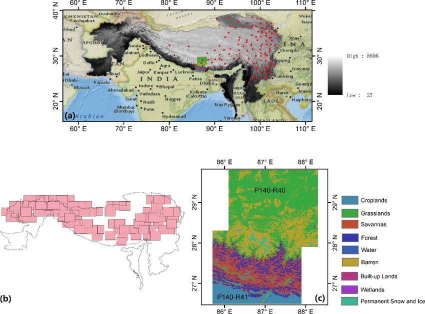
4262                                      X. Wu et al.: Evaluation of snow extent time series in the Hindu Kush Himalayas

ment decisions, and investigating climate change impacts on        the performance of the AVHRR GAC snow product needs
environmental variables (Arsenault et al., 2014; Sun et al.,       to be extensively evaluated, especially over the HKH re-
2020).                                                             gion which is highly sensitive to climate change. This paper
   The Hindu Kush Himalayan (HKH) region, which is often           presents the validation of the AVHRR GAC snow product
called the freshwater tower of Asia, comprises the highest         over the HKH area during snow seasons. Of particular im-
concentration of snow outside the polar regions. The snow          portance is validating the temporal performance of the prod-
cover of this area plays a crucial role in the water supply of     uct (i.e., different platform operated over the entire dataset
several major Asian rivers (Immerzeel et al., 2009). On the        period). To this end, the first validation was carried out us-
other hand, the HKH region is of special interest due to its       ing 118 in situ stations’ measurements. The correlation be-
large area, rich diversity of climates, hydrology, ecology, and    tween spatial products and “point” measurements depends
biology (Wester et al., 2019). Variations in snow cover af-        strongly on the selected snow depth. Therefore, the influ-
fect the precipitation, near-ground air temperature, and sum-      ence of snow depth on the accuracy of the product was also
mer monsoon in Eurasia and across the Northern Hemisphere          investigated. Considering that the HKH region features dis-
(Hao et al., 2018). Given the fact that the HKH region is par-     tinct characteristics of snow cover with shallowness, patch-
ticularly sensitive to climate change and thus shows strong        iness, and frequent short duration ephemeral snow (Qin et
interannual variability, reliable daily snow-cover data over a     al., 2006), in situ site measurements alone are not enough to
long time series across this area are in great demand.             characterize its accuracy. A multi-scale validation and com-
   Optical satellite data provide important data sources for       parison strategy is highly needed to assess its accuracy over
snow-cover retrieval through the contrasting spectral behav-       greater spatial extent and elevation ranges. Within this vali-
ior of snow relative to other natural surfaces in the visi-        dation framework, the influences of land-cover types, eleva-
ble and middle-infrared regions (Tedesco, 2014; Zhou et al.,       tions, aspects, slopes, and topographies on the accuracy of
2013). The global spatial coverage of satellite data makes it      AVHRR GAC snow were also explored. Finally, the MODIS
an efficient data source to improve our knowledge of snow-         snow maps were also introduced to conduct a comparison
cover dynamics (Siljamo and Hyvärinen, 2011; Solberg et            between the well-validated MODIS product and the new
al., 2010). Many satellites have been used to generate snow-       AVHRR GAC snow product. Section 2 describes the study
cover products at various spatial and temporal resolutions,        area and data. The validation methodology is explained in
such as AMSR-E (Tedesco and Jeyaratnam, 2016), MODIS               Sect. 3. The performance of the AVHRR GAC snow dataset
(Riggs et al., 2016a), AVHRR (Advanced Very High Reso-             is presented and discussed in Sect. 4. A brief conclusion is
lution Radiometer; Shan et al., 2016), VIIRS (Riggs et al.,        presented at the end.
2016b), and Landsat (Rosenthal and Dozier, 1996). In par-
ticular, new generation satellite sensors (e.g., MODIS, VI-
IRS) generally show an advantage over old sensors such             2     Study area and data
as AVHRR and TM/ETM (Thematic Mapper and Enhanced
Thematic Mapper) which suffer from significant saturation          2.1    Study area
over snow in the visible channels (WMO, 2012). Neverthe-
less, AVHRR offers the unique opportunity to generate a con-       The HKH region covers a mountainous region of more than
sistent snow product over a 30-year normal climate period          4 million km2 within the geographic area between about 16
(IPCC, 2013) and thus remains vitally important. In response       to 40◦ N latitude and 60 to 105◦ E longitude. It extends
to the systematic observation requirements of the Global Cli-      across all or parts of eight countries, namely Afghanistan,
mate Observing System (GCOS), the ESA Climate Change               Bangladesh, Bhutan, China, India, Myanmar, Nepal, and
Initiative (CCI) has emphasized the necessity of generat-          Pakistan (You et al., 2017). Moreover, it contains the high-
ing consistent, high-quality long-term datasets over the last      est concentration of snow and ice outside the polar regions
30 years as a timely contribution to the ECV (Essential Cli-       and is thus referred to as the “Third Pole” (Wester et al.,
mate Variable) databases. For this demand, a global time se-       2019). This region is one of the most dynamic, fragile, and
ries of daily fractional snow-cover products has been gener-       complex mountain systems in the world due to the rich diver-
ated from AVHRR GAC (global area coverage) data (Naegeli           sity of climatic, hydrological, and ecological characteristics.
et al., 2021). This snow dataset is unique as it spans 4 decades   The climate conditions range from tropical (< 500 m a.s.l.) to
and thus provides information about an ECV at climate-             high alpine and nival zones (> 6000 m a.s.l.), with a principal
relevant timescales.                                               vertical vegetation regime composed of tropical and subtrop-
   Nevertheless, there are many factors, such as data process-     ical rainforests, temperate broadleaf, deciduous, or mixed
ing (e.g., calibration, geocoding) and the accuracy of cloud       forests, temperate coniferous forests, alpine moist and dry
masking, atmospheric constituents, topographic effects, bidi-      scrub, meadows, and desert steppe (Guangwei, 2002). The
rectional reflectance distribution function (BRDF), and the        main land cover of this region is rangeland, which covers
limitations of snow-cover retrieval algorithms, influencing        approximately 54 % of the total area. Agriculture and for-
the accuracy of the AVHRR GAC snow-cover extent. Hence,            est are also present, accounting for 26 % and 14 % of this

The Cryosphere, 15, 4261–4279, 2021                                                    https://doi.org/10.5194/tc-15-4261-2021
X. Wu et al.: Evaluation of snow extent time series in the Hindu Kush Himalayas                                           4263

region, respectively. A total of 5 % of this region is perma-    of the canopy, as well as on ground below the canopy, by
nent snow and glaciers, and 1 % is water bodies (Ning et al.,    taking the canopy density into account. Here, we focus on
2014; Wester et al., 2019). Snowmelt is considered to be a       the latter variable as this is most suitable for the comparison
key source of water supply in the HKH range, and the ability     with in situ stations.
of snow products to quantify snow storage and melt is thus          To reduce the effect of cloud coverage, a temporal filter
critical for the management of water resources (Foster et al.,   of ±3 d for each individual snow-cover observation was ap-
2011).                                                           plied based on Foppa and Seiz (2012). The AVHRR GAC
   The validation based on in situ stations covers mainly        FCDR snow-cover product comprises only one longer data
the eastern part of the HKH region (Fig. 1a). To demon-          gap of 92 d between November 1994 and January 1995, re-
strate the accuracy of the AVHRR snow product over the           sulting in a 99 % data coverage over the entire study period
whole area, Landsat data covering the entire region were in-     of 38 years. In this study, we will focus on the evaluation of
troduced to conduct a multi-scale validation (Fig. 1b). Fur-     raw daily retrieval of AVHRR GAC snow extent (denoted by
thermore, in order to explore its performance in high de-        “AVHRR_Raw”) since additional uncertainty will be intro-
tail for a wide range of conditions (e.g., elevation, topog-     duced with the gap-filling process.
raphy, and land cover), validation against Landsat TM data
was also performed in detail using two tiles of Landsat          2.3     Validation datasets
data (path 140, rows 40 and 41, denoted as “P140-R40/41”)
(Fig. 1c), covering a diverse region on the Nepal/Tibet bor-     2.3.1    In situ snow depth measurements
der centered around Mount Everest. This region was cho-
sen because it contains the greatest elevation range in the      In situ data were provided by the China Meteorological Ad-
Himalayas. The northernmost part of this region are areas        ministration (https://data.cma.cn/en, last access: 30 Octo-
on the Tibetan plateau exceeding 6000 m a.s.l. where vegeta-     ber 2019). Daily snow depth (SD) measurements (118 · 365)
tion change is occurring rapidly (Qiu, 2016). Furthermore, it    are obtained from 118 stations located at different elevations
covers a broad range of climatic conditions (Bookhagen and       ranging from 776 to 8530 m above sea level. SD was usu-
Burbank, 2006). Therefore, this region is a microcosm of the     ally measured over a large flat area using rulers at 08:00 LT
range of conditions experienced across the wide HKH region       (UTC+8) every day. Three measurements were made at least
and thus provides a good point for investigating snow extent     10 m away, and their mathematical mean was used as the
accuracy under different conditions (Anderson et al., 2020).     daily snow depth. In particular, if snowfall occurred after
                                                                 08:00, a second measurement at 14:00 or a third measure-
2.2   AVHRR GAC snow extent retrieval                            ment at 20:00 were needed depending on the time of snow-
                                                                 fall. The data were rounded to the nearest centimeter. Thus,
The AVHRR GAC snow-cover extent time series version 1            SD less than 0.5 cm would be labeled as 0 cm in the record.
derived in the frame of the ESA CCI+ Snow project is the         Detailed quality control was made to flag suspicious values.
most recent long-term global snow-cover product available        The period from 1982 to 2013 was used to prove the temporal
(Naegeli et al., 2021). It covers the period 1982–2019 at a      consistency of the AVHRR GAC snow-cover extent product.
daily temporal and 0.05◦ spatial resolution. The product is
based on the Fundamental Climate Data Record (FCDR)              2.3.2    Landsat TM/ETM data and processing
consisting of daily composites of AVHRR GAC data
(https://doi.org/10.5676/DWD/ESA_Cloud_cci/AVHRR-                Landsat data were introduced for two purposes: (i) to check
PM/V003) produced in the ESA CCI Cloud project (Stengel          the spatial consistency between AVHRR GAC snow and
et al., 2020). The data were preprocessed with an improved       Landsat-based snow based on 197 scenes covering the whole
geocoding and an inter-channel and inter-sensor calibration      HKH region and (ii) to explore the factors (e.g., eleva-
using PyGAC (Devasthale et al., 2017). The snow-cover            tion, topography, and land cover) influencing the accuracy
extent retrieval method was developed and improved based         of AVHRR GAC snow based on P140-R40/41. To mitigate
on the ESA GlobSnow approach described by Metsämäki              the effect of clouds, the validation over P140-R40/41 was
et al. (2015) and complemented with a pre-classification         restricted to clear-sky (cloud no more than 10 %) scenes of
module. Alongside the daily reflectance and brightness           Landsat 5 TM during snow seasons (46 · 2 scenes from 1984
temperature information, an excellent cloud mask including       until 2013; downloaded from https://glovis.usgs.gov/, last ac-
pixel-based uncertainty information is provided (Stengel et      cess: 30 April 2020). The validation over the whole HKH
al., 2017, 2020). All cloud-free pixels are then used for the    region was restricted to Landsat clear-sky scenes from 1999
snow extent mapping using spectral bands centered at about       to 2018 (197 scenes) (Fig. 1b). Level-1 Precision and Ter-
630 nm and 1.61 µm (channel 3a or the reflective part of         rain Correction (L1TP) data were selected since they have
channel 3b) and an emissive band centered at about 10.8 µm.      been radiometrically and geometrically corrected. Following
The water bodies, permanent ice bodies, and missing values       the recommendation of Metsämäki et al. (2015), the frac-
are flagged. SCAmod retrieves both the snow cover on top         tional snow method by Salomonson and Appel (2006) was

https://doi.org/10.5194/tc-15-4261-2021                                                The Cryosphere, 15, 4261–4279, 2021
4264 X. Wu et al.: Evaluation of snow extent time series in the Hindu Kush Himalayas
Figure 1. (a) The HKH region and the distribution of in situ station locations (red dots). (b) The distribution of Landsat scenes available over
the whole HKH region. (c) Land-cover type of the P140-R40/41 region of interest which corresponds to Landsat path 140, rows 41 and 42,
on the Nepal–Tibet border.
employed to generate reference FSC (fractional snow cover) 2.3.3 MODIS snow-cover product
from Landsat TM/ETM imagery. This method is originally
designed for MODIS FSC products, with a mean absolute er-
The Terra MODIS Level 3, Collection 6, 500 m daily
ror of less than 10 % (Salomonson and Appel, 2004). In this
snow-cover products (MOD10A1) (Hall and Riggs, 2016)
paper, we assumed that such an accuracy can be achieved
over the HKH region from 2000 to 2013 were obtained
with higher resolution data. Bands 2 (0.53–0.61 µm) and
through Google Earth Engine (GEE). The MODIS snow
5 (1.55–1.75 µm) were used to provide NDSI (normalized
detection algorithm also uses NDSI and other test criteria
difference snow index) estimates (Eq. 1), and then the Sa-
(Riggs et al., 2016a). Instead of directly providing binary
lomonson and Appel scaling (Eq. 2) is applied. These high-
snow-covered area (SCA) and FSC, version V006 provides
resolution data were then projected to a geographic projec-
NDSI_Snow_Cover and NDSI. The former is reported in the
tion and aggregated to AVHRR GAC pixel scale using the
range of 0–100 with other features identified by mask val-
area-weighted average of contributing pixels to “simulate”
ues, while the latter represents the real NDSI values multi-
the reference FSC estimates at the AVHRR GAC pixel scale.
plied by 10 000, which is calculated for all pixels (Riggs et
al., 2016a). This treatment provides more information and
NDSI = (B2 − B5)/(B2 + B5), (1) great flexibility to enhance the accuracy of the product be-
FSC = −0.01 + 1.45 × NDSI, (2) cause the NDSI range is not necessarily restricted to 0.4 to
1.0 for snow detection. Actually, NDSI_Snow_Cover func-
where B2 and B5 denote the spectral bands 2 and 5, respec- tions very similarly to FSC in version V005 since it can be
tively. linked using the equation of FSC = −0.01 + 1.45 × NDSI.
The Cryosphere, 15, 4261–4279, 2021 https://doi.org/10.5194/tc-15-4261-2021X. Wu et al.: Evaluation of snow extent time series in the Hindu Kush Himalayas 4265
Figure 2. AVHRR GAC raw (a, b) and gap-filled (c, d) snow cover for the entire HKH region in March 1984 (a, c) and March 2010 (b, d).
Compared to the previous version, version V006 made great Geosphere–Biosphere Programme (IGBP) of the MCD12Q1
improvements on atmospheric correction, cloud cover, and mosaic was used to investigate the difference in accuracy
quality index. Furthermore, the algorithm takes a pixel’s el- over different land-cover types. It includes 11 types of nat-
evation into account, which is especially important for ele- ural vegetation, 3 types of developed and mosaic lands, and
vated snow-covered surfaces in spring. In order to avoid a 3 types of non-vegetated lands, which have been reclassi-
spatial-scale mismatch between AVHRR and MODIS pix- fied into nine major classes: forest, grassland, savannas, crop-
els, MOD10A1 was reprojected to a geographic projection lands, built-up lands, barren, permanent snow and ice, water
and aggregated to AVHRR GAC pixel scale using the area- body, and wetlands. In order to match with the pixel size of
weighted average of contributing pixels. AVHRR GAC snow, the MCD12Q1 was resampled to 0.05◦
spatial resolution with the nearest neighbor interpolation.
2.3.4 Auxiliary data
The digital elevation model (DEM) information was obtained 3 Methods
from the SRTM (Shuttle Radar Topography Mission) dataset,
which provides a nearly global coverage with a spatial reso- AVHRR GAC snow extent was evaluated from several as-
lution of 90 m. In this study, the elevation, slope, aspect, and pects. The validation based on in situ sites aims to prove the
topographical variability were derived using this dataset in long-term consistency since in situ stations provide valuable
order to investigate their influences on the accuracy of the long time series measurements, while the comparison with
AVHRR GAC snow extent product. The topographical vari- Landsat and MODIS snow is focused on their spatial consis-
ability within a certain AVHRR GAC pixel was determined tency and the in-depth analysis of influential factors (eleva-
by calculating the standard deviation of elevations of all sub- tion, topography, and land cover). The validation strategy is
pixels within its spatial extent, while the elevation, slope, and briefly summarized in Table 1.
aspect were resampled to match the resolution of the AVHRR
GAC snow dataset. 3.1 Binary validation based on in situ data
The MODIS Terra/Aqua Combined Annual Level 3
Global 500 m Collection 6 land-cover dataset (MCD12Q1) Although the validation based on in situ sites leaves issues
was generated using a supervised classification methodol- of scale unresolved and therefore likely accompanied by un-
ogy (Friedl et al., 2010). In this study, the International certainties, in situ observations provide the only source to
https://doi.org/10.5194/tc-15-4261-2021 The Cryosphere, 15, 4261–4279, 20214266 X. Wu et al.: Evaluation of snow extent time series in the Hindu Kush Himalayas
Table 1. Validation strategy: data and purpose.
Data source Variable(s) Application purpose Validation purpose
In situ stations Snow depth Binary (snow/no snow) valida- Temporal consistency but spa-
tion of snow cover tially limited, and dependence
on snow depth
MOD10A1 Snow cover Quantitative comparison of Relative comparison to investi-
snow cover gate general performance
Landsat east/west Snow cover Absolute comparison of snow- Great spatial and patchy tempo-
cover extent ral coverage
Landsat P140-R40/41 Snow cover Absolute comparison of snow- Limited spatial and temporal
cover extent coverage but great variability in
elevation, topography, and land
cover
High- and medium- Snow cover, land cover, eleva- – Dependency on land-cover
resolution satellite tion, topography (aspect, slope) type, topography, and elevation
images (Landsat,
MODIS, SRTM DEM)
validate the time series AVHRR GAC snow extent over this as snow, it is labeled as zero (d); if the snow product indi-
long period. Since there is no reliable way to convert SD to cates the pixel as snow, but the reference data does not, it is
FSC, both FSC and SD information were converted to binary marked as false (b); and if the opposite occurs, it is indicated
information by applying appropriate thresholds, respectively. as a miss (c) (Hüsler et al., 2012; Siljamo et al., 2011).
Different thresholds have been suggested for in situ SD mea- Based on these measures, indicators such as accuracy
surements to determine whether the associated pixel is cov- (ACC), Heidke skill score (HSS), and bias (Bias) were de-
ered by snow, ranging from 0 to 5 cm (Parajka et al., 2012; termined (Eqs. 3–5) (Hüsler et al., 2012). ACC denotes the
Hori et al., 2017; Hao et al., 2019; Huang et al., 2018; Liu et percentage of correctly classified pixels divided by the total
al., 2018; Zhang et al., 2019; Gascoin et al., 2019). Therefore, number of pixels. ACC values closer to 1 denotes a perfect
the sensitivity of thresholds was tested by computing accu- agreement between the snow product and the reference data,
racy metrics with SD increasing from 1 to 5 cm. The FSC while a value of 0 corresponds to complete disagreement.
maps were transferred from fractional to binary snow infor- However, it is strongly influenced by the most frequent cat-
mation by applying a threshold of FSC ≥ 50 %. The value egory (i.e., in summer) (Hüsler et al., 2012) and thus ideally
of 50 % is widely used and accepted in snow-cover detec- requires an equal distribution of categories. Hence, we con-
tion (Wunderle et al., 2016; Mir et al., 2015; Crawford, 2015; fine our accuracy assessment to the snow season (from Oc-
Marchane et al., 2015; Hall and Riggs, 2007). tober to March) only, a limitation that was implemented in
Concerning the comparison of spatial satellite data with other studies as well (Yang et al., 2015; Gafurov et al., 2012;
in situ measurements, a point-wise comparison was imple- Hüsler et al., 2012; Huang et al., 2011). The HSS and Bias
mented. To relate in situ “point” measurements with AVHRR provide refined measures in cases when the frequency distri-
GAC “area” snow information, both the center pixel contain- bution within the validation subsets is not equal. The former
ing the in situ point measurement and the 3 × 3 pixels cen- describes the proportion of pixels correctly classified over
tered around this point were tested, respectively. This treat- the number that was correct by chance in the total absence of
ment took into consideration the influence of data noise, geo- skill. Negative values indicate that the chance performance
metric mismatch, and spatial heterogeneity. Furthermore, the is better, 0 represents no skill, and a perfect performance ob-
absence or presence of snow indicated by in situ observations tains an HSS of 1 (Hüsler et al., 2012). It is generally true that
is assumed to be representative of at least a 3 × 3 pixel area, a value above 0.3 denotes a relatively good score for a reason-
but this depends on topography. Consequently, there are al- ably sized sample for the binary forecast (Singh, 2015). The
together 10 combination cases for accuracy assessment (Ta- Bias, described by the ratio of the number of snow-covered
ble 2). pixels to the number of reference data pixels, is a relative
The 2 × 2 contingency table statistics (Table 3) were uti- measure to detect overestimation (value is higher than 1) or
lized to indicate the quality of the snow product. If both ref- underestimation of snow (value is less than 1). Unbiased re-
erence data and the snow product identified the pixel as snow,
it is labeled as a hit (a); if neither of them indicated the pixel
The Cryosphere, 15, 4261–4279, 2021 https://doi.org/10.5194/tc-15-4261-2021X. Wu et al.: Evaluation of snow extent time series in the Hindu Kush Himalayas 4267
Table 2. A short summary of all the combinations of thresholds.
Cases Combinations Cases Combinations
Case1 SD ≥ 1 cm, center pixel Case6 SD ≥ 1 cm, 3 × 3 pixels
Case2 SD ≥ 2 cm, center pixel Case7 SD ≥ 2 cm, 3 × 3 pixels
Case3 SD ≥ 3 cm, center pixel Case8 SD ≥ 3 cm, 3 × 3 pixels
Case4 SD ≥ 4 cm, center pixel Case9 SD ≥ 4 cm, 3 × 3 pixels
Case5 SD ≥ 5 cm, center pixel Case10 SD ≥ 5 cm, 3 × 3 pixels
Table 3. Contingency table used to determine probability of detec- (RMSE), mean bias (mBias), and the coefficient of correla-
tion and bias. tion (R) were derived through the scene-by-scene compari-
son.
Reference data (in situ)
Snow product Yes No
3.2 Multi-scale validation based on high-resolution
(e.g., AVHRR Yes a: hit b: false a+b snow-cover maps
GAC or
MODIS) In order to evaluate AVHRR GAC snow at a broader spa-
No c: miss d: zero c+d tial scale, Landsat TM/ETM aggregated FSC was used as the
a+c b+d n =a+b+c+d reference. Snow-free values are treated as 0 % snow, and a
fully snow-covered pixel is assigned 100 % snow. The vali-
dation was conducted from two aspects: (i) one is based on
sults should have a value of 1. 197 scenes covering the whole HKH region in order to in-
crease the spatial coverage of validation, and (ii) the other
a+d is based on 46 · 2 scenes over P140-R40/41 in order to make
ACC = (3)
a+b+c+d a detailed analysis of the factors (e.g., elevation, topography,
2(ad − bc) and land cover) influencing the accuracy of the AVHRR snow
HSS = (4) dataset.
(a + c) (c + d) + (a + b)(b + d)
a+b
Bias = (5)
a+c 4 Results and discussion
The validation follows two types of strategies. First, the 4.1 The validation based on in situ data
snow-cover data time series of satellite and in situ station
were compared, resulting in accuracy indicators over each 4.1.1 Snow depths and pixel threshold sensitivity
station. This validation allows us to check the spatial diver- analysis
gence of accuracy within different sites, as well as the effect
of land cover on the accuracy of satellite-derived snow infor- To test the sensitivity of the in situ SD threshold for the snow-
mation. Second, the snow data of all in situ sites were com- cover detection, the overall accuracy metrics were computed
bined together for validation of AVHRR GAC snow on the by combining data of all in situ sites throughout the study pe-
daily basis. In this way, the long-term temporal consistency riod (from 1982 to 2013 for the AVHRR-GAC-derived snow
of accuracy can be evaluated. Additionally, in order to assess and from 2000 to 2013 for MOD10A1). The variations in
the product performance with respect to the temporal vari- Bias, ACC, and HSS with all the threshold combinations (Ta-
ability in snow cover, the binary metrics are summarized and ble 2) are shown in Fig. 3.
analyzed for each month. An analysis of increase/decrease in As shown in Fig. 3a, an SD threshold of 2 cm (case2)
accuracy with respect to FSC and SD was also included to maximizes the overall accuracy of the AVHRR GAC snow-
explore the influence of smaller snow patches on the accu- cover dataset. With the further increase in SD threshold, the
racy. AVHRR GAC snow detected will be seriously overestimated.
Finally, in order to check the relative performance of This indicates the presence of snow can be best detected by
AVHRR GAC snow to the well-used MODIS product, the AVHRR GAC dataset for in situ snow depth measure-
MOD10A1 V006 was also evaluated with in situ station data ment of 2 cm. Furthermore, the increasing rate of ACC and
following the same method. It is expected that the major dif- decreasing rate of HSS are the highest between the 1 and
ference in their performance is either due to the quality of 2 cm SD thresholds, and it flattens for greater SD thresholds.
the applied processing and snow-cover retrieval algorithms When it comes to the influences of geometric mismatch or
or the general satellite data characteristics. As for the com- spatial heterogeneity (center pixel versus 3 × 3 pixels; Ta-
parison of their absolute values, the root mean square error ble 2), they show significant effects on both the magnitude
https://doi.org/10.5194/tc-15-4261-2021 The Cryosphere, 15, 4261–4279, 20214268 X. Wu et al.: Evaluation of snow extent time series in the Hindu Kush Himalayas
and the variation trend of these accuracy indicators. But such As shown in Fig. 4, it can be seen that MODIS snow is
effects are not fixed and vary by satellite datasets and ac- inferior to AVHRR GAC snow regarding the magnitude of
curacy indicators (Fig. 3). For this reason, we chose case2 ACC and its temporal consistency. Furthermore, its HSS is
(SD ≥ 2 cm, center pixel) as the optimum threshold combi- consistently smaller than that of AVHRR GAC snow. Never-
nation for the evaluation of the AVHRR GAC snow dataset. theless, its temporal stability is slightly better than AVHRR
For consistency, this choice was also used for the comparison GAC snow since the HSS of MODIS almost stays constant
of the performance of MODIS with in situ data. over time. When it comes to Bias, MODIS snow shows a
As seen from Fig. 3a, AVHRR snow datasets show dis- more serious overestimation than AVHRR GAC snow but
tinct advantages over MODIS snow regarding the Bias value. comparable temporal stabilities to the latter.
The former shows biases of 0.94 and 1.03 for the AVHRR In order to highlight the performance of AVHRR GAC
raw snow and gap-filled snow, respectively, while the latter snow in different months, the temporal variations in ACC,
is seriously overestimated with the bias of 1.74. Neverthe- HSS, and Bias over different months are presented (Fig. 5).
less, the three datasets show comparable ACC, with the val- From Fig. 5a, it can be seen that ACC of AVHRR GAC snow
ues of 0.94, 0.92, and 0.94 for AVHRR raw snow, AVHRR is over 0.85 for all months and even above 0.90 for October.
gap-filled snow, and MODIS snow datasets, respectively. The Nevertheless, both the temporal variation trend and the mag-
HSSs of the three datasets are reasonable, with the values nitude of ACC show differences from month to month. It is
larger than 0.3. MODIS snow shows the largest HSS of 0.35, clear that the AVHRR GAC snow shows the highest ACC in
followed by AVHRR raw snow with an HSS of 0.34. The October and lowest ACC in January, but the temporal stabil-
AVHRR gap-filled snow-cover dataset ranks last, with the ity of ACC is best in November and worst in January and De-
smallest HSS of 0.31. From the above results, it can be found cember. It is interesting that the results tend to polarize into
that the AVHRR raw dataset performs slightly better than two groups: ACC for January through March and ACC for
the AVHRR gap-filled dataset with respect to the agreement October through December. Generally, ACC in the former
with in situ sites and the algorithm performance (skill). This group is smaller than those in the latter group. It is notewor-
is reasonable since additional uncertainty was introduced in thy that ACC after 2000 is generally larger and more stable
the gap-filling process. For this reason, we will only focus on than those in earlier years on the monthly scale (Fig. 5a), in-
AVHRR raw snow for further analysis. Generally, AVHRR dicating the better accuracy and consistency of the younger
raw snow is comparable with MODIS snow when ACC and satellite platforms after 2000. Compared to AVHRR GAC
HSS are focused. snow, the ACC of MODIS snow consistently shows large
temporal variations for all months, and there is no month
that shows advantages over others regarding the magnitude
4.1.2 The temporal consistency of quality indicators
and temporal stability of ACC (Fig. 5b).
The HSS for different months are larger than 0.4 through-
From Fig. 4, it can be seen that the interannual variability out the time series, but large differences of the magnitude and
in these accuracy metrics is evident, especially for ACC and temporal stability exist between different months (Fig. 5c).
HSS. In the time series of AVHRR GAC snow, ACC is basi- Similar to ACC, the AVHRR GAC snow generally shows the
cally distributed between about 88 % and 92 % (Fig. 4a). An largest HSS in October for most of the time. Furthermore,
obvious increase in ACC can be observed from 1982 to 1985, the HSS in October shows a similar temporal variation trend
followed by a decrease in ACC from 1985 to 1992. Then an with the overall temporal trend of HSS in Fig. 4b. Among
increasing trend of ACC occurs from 1992 to 2000. From all the months, the HSS in December shows the largest tem-
2000 to 2010, ACC is relatively stable with time. But af- poral variations, featured by the highest HSS from 1990 to
ter 2010, an increasing trend reappears. Differently from the 2000 and the lowest HSS from 2005 to the end. The HSS
previous assessments, the ACC of the AVHRR snow datasets in January through March shows relatively smaller temporal
at the beginning of the time series (1982–2000) is slightly variations than those in October through December. Regard-
worse than the end of the time series (2000–2013) regard- ing the magnitude of HSS, the different rank of these months
ing the magnitude of ACC and its temporal consistency. The during different periods may be associated with the shift of
HSS shows a different behavior compared to ACC (Fig. 4b), snow-cover phenology due to interannual variability intensi-
which increases slightly and monotonously from 0.45 at the fied by global warming. Unlike AVHRR GAC snow, MODIS
beginning to about 0.48 at the end of the time series. This snow shows larger HSSs in January and February (Fig. 5d).
further indicates that the performance of AVHRR snow con- Furthermore, the temporal variations in HSS are more signif-
tinues to improve with time. Nevertheless, the improvements icant than AVHRR GAC during the same period.
of the performance of AVHRR GAC snow do not occur in Although the AVHRR GAC snow shows the best perfor-
the Bias (Fig. 4c). The Bias shows the best performance from mance in October regarding the magnitude of ACC and HSS,
1990 to 2000, with relatively stable values around 1. But dur- it shows serious overestimation in this month (Fig. 5e). In
ing other time periods, relatively large fluctuations appear, particular, AVHRR GAC snow generally overestimates snow
and it generally overestimates snow during these periods. in February, March, October, and November. By contrast, it
The Cryosphere, 15, 4261–4279, 2021 https://doi.org/10.5194/tc-15-4261-2021X. Wu et al.: Evaluation of snow extent time series in the Hindu Kush Himalayas 4269
Figure 3. Sensitivity analysis of product accuracy related to snow depth thresholds of the in situ station data. The overall error is a spatiotem-
porally integrated statistical measure.
either slightly overestimates or underestimates snow in De-
cember and January, with the bias distributed around 1. This
result is understandable because during December and Jan-
uary, snow coverage tends to be dense and spatially continu-
ous, which results in unbiased estimation. By contrast, during
February, March, October, and November, snow cover tends
to be patchy, and AVHRR GAC data are more able to detect
snow than in situ point observations due to the large pixel
coverage. MODIS snow consistently overestimates snow in
different months and shows larger temporal variations than
AVHRR GAC snow (Fig. 5f).
From the results above, it can be concluded that the
AVHRR GAC snow dataset performs variably throughout
the course of the year, which may be related to the different
amounts of snow in the HKH region. Generally, the magni-
tudes of ACC and HSS are largest in October and smallest in
January. But the temporal stability of ACC is best in Novem-
ber and worst in January and December, while that of HSS
is worst in December. The results of Bias provide different
perspectives for the performance of AVHRR GAC snow. It
generally overestimates snow in February, March, October,
and November. By contrast, unbiased estimation is likely to
occur in December and January. Compared to AVHRR snow
datasets, the interannual variability in ACC, HSS, and Bias
of the MODIS snow product in different months is generally
stronger (Fig. 5).
Figure 4. The time series (denoted by the dashed lines) of ACC,
4.1.3 The spatial consistency of quality indicators
HSS, and Bias for AVHRR raw and MODIS snow data during the
investigated period. A simple moving average with a box dimension
of n = 30 was applied to the time series in order to reduce the noise Figure 6 show the boxplots of the validation metric derived
and uncover patterns in the data. The solid lines represent the fitted from each in situ station, with the aim of revealing their
trend of these accuracy indicators. spatial variability. It can be observed that the spatial vari-
ability in these validation metrics widely exists given their
dispersed distribution. The maximum of ACC even reaches
https://doi.org/10.5194/tc-15-4261-2021 The Cryosphere, 15, 4261–4279, 20214270 X. Wu et al.: Evaluation of snow extent time series in the Hindu Kush Himalayas
Figure 5. The temporal behavior of ACC for AVHRR raw and MODIS snow data in different months (indicated by the different colored
lines) during the snow season. The solid-colored lines represent the fitted trend of these accuracy indicators for different months.
0.99 for the AVHRR snow datasets, while the minimum val- MODIS show similar responses. The highest ACC occurred
ues are close to 0.76 (Fig. 6a). Similarly, HSS also shows when SD=0 cm, which is followed by SD = 1 cm. When
a dispersed distribution for the AVHRR snow datasets. The SD ≥ 2 cm, the ACC decreases significantly. The threshold
AVHRR raw dataset ranges from 0.2 to 0.39 with min–max of 2 cm which transforms in situ SD measurements to snow-
values of 0.01 to about 0.68 (Fig. 6b). Likewise, the bias is lo- cover or snow-free information is partly responsible for this
cated around 0.51–1.6 with min–max values of 0.05 and 2.89 result. Another cause of this phenomenon is the representa-
for the AVHRR dataset (Fig. 6c). These results are under- tiveness of the point-scale in situ observation compared with
standable because the performance of satellite snow datasets satellite observation on a larger pixel scale. When SD was
is affected by many factors. Despite the awareness of spatial less than 2 cm, it is more likely that snowfall events only oc-
variability in these validation metrics, the degree of variabil- curred over a limited area of the satellite pixel. In this con-
ity depends on satellite datasets and metrics. The HSS and dition, satellite snow datasets are more likely to classify the
Bias of the MODIS snow dataset are more divergent than the pixel as snow-free, which would increase the agreement be-
AVHRR raw snow dataset (Fig. 6). tween satellite and in situ observations. Despite the decrease
in ACC when SD ≥ 2 cm (compared to SD < 2 cm), the ACC
4.1.4 The potential factors influencing accuracy of various snow datasets clearly shows an increasing trend
with increasing SD. It is understandable since, with increas-
Following the early study (Klein and Barnett, 2003), the ef- ing SD, the satellite pixel is more likely to be entirely covered
fect of SD on the accuracy of satellite snow datasets was by snow, and the agreement between satellite and in situ ob-
evaluated (Fig. 7a). Observed SD was divided into six cat- servations, as a result, increases. In general, SD was shown
egories: SD = 0, 1, 2, 3, 4, and 5 cm. It is obvious that the to affect the overall agreement of satellite snow datasets, and
ACC of the two satellite snow datasets based on AVHRR and their accuracies increase with increasing SD in the situation
The Cryosphere, 15, 4261–4279, 2021 https://doi.org/10.5194/tc-15-4261-2021X. Wu et al.: Evaluation of snow extent time series in the Hindu Kush Himalayas 4271
Figure 6. The boxplots of ACC (a), HSS (b), and Bias (c) for AVHRR raw and MODIS snow data throughout the sites. The numbers around
the plots indicate the minimum, lower quartile, median, upper quartile, and maximum of the boxplots.
when the in situ site indicates snow-cover information, which As seen in Fig. 7a, we can find that the accuracy of the
is in line with previous studies (Zhou et al., 2013; Wang et AVHRR snow datasets is larger than the MODIS snow prod-
al., 2009). uct when SD ≤ 1 cm but consistently smaller than MODIS
The effect of FSC on the accuracy of satellite snow snow at each SD when SD ≥ 2 cm. This means that in snow-
datasets was checked in Fig. 7b. FSC was grouped into five free or very thin snow conditions, the AVHRR snow datasets
categories using the ranges of 0 %–20 %, 20 %–40 %, 40 %– are less misclassified than the MODIS snow product, but
60 %, 60 %–80 %, and 80 %–100 %. Likewise, the ACC in contrast, in snow-covered conditions, although the three
of the AVHRR and MODIS snow datasets shows a sim- datasets all reveal an increase in ACC with increasing SD,
ilar response to FSC. The highest ACC was found when the MODIS snow product is more reliable and correctly clas-
FSC ≤ 20 %, followed by 20 % < FSC ≤ 40 %. This is also sified. The discrepancies between them mainly result from
partly caused by the threshold (FSC ≥ 50 %) applied to FSC the different spatial scale of the pixel. From Fig. 7b, it be-
maps to transfer fractional to binary snow information and comes apparent that accuracies of the AVHRR snow datasets
partly caused by the spatial representativeness of in situ sites. are slightly lower than the MODIS product for each level of
When only a small part of the pixel is covered by snow, in situ FSC when FSC ≤ 60 % but larger than the MODIS product
sites are more likely covered by very thin snow or not cov- when FSC > 60 %. This phenomenon is related to the differ-
ered by snow. Consequently, in situ sites are more likely to ent degrees of spatial representativeness of in situ sites rela-
be indicated as snow-free, which increases the agreement be- tive to different pixel scales.
tween in situ and satellite observations. In the situation of Figure 8a and b present the distribution of ACC for two
40 % < FSC ≤ 60 %, ACC decreases significantly. This oc- satellite snow datasets against in situ site observations over
curs because part of the satellite data in this group indicates different elevation regions (five classes) and land-cover types
snow cover using the threshold FSC ≥ 50 %, but there ap- (four types), respectively. It is generally thought that coarse-
pears a strong possibility that the in situ site is not covered pixel satellite snow products perform better at higher eleva-
by snow or only covered by very thin snow. For the case of tions due to the continuous and thick snow cover (Yang et al.,
60 % < FSC ≤ 80 %, all satellite data in this group indicate 2011). Nevertheless, the ACC over the HKH region shows
snow cover, but there remains a very real risk that the in situ different phenomena. The two satellite snow products con-
site is not covered by snow or only covered by very thin sistently show larger ACC over slightly lower elevations than
snow. As a result, the agreement between them further de- those over higher elevations. Nevertheless, an exception can
creases. With the further increase in FSC, the possibility that be found in the elevation region of 3500–4500 m, where the
in situ sites indicate snow cover also increases. Thus, ACC ACC of the two datasets is the lowest over the whole HKH
increases in the situation of 80 % < FSC ≤ 100. From these region. Furthermore, the ACC over these elevation regions is
results, it is concluded that FSC affects the overall agree- the most divergent, demonstrating that the accuracy of snow
ment between satellite snow datasets and in situ observations. product within this range is more likely to be affected by
In the condition that satellite data indicate snow-free, ACC other factors. It is noteworthy that the MODIS snow product
decreases with increasing FSC. By contrast, in the case of slightly outperforms the AVHRR snow dataset over different
satellite data indicating snow cover, ACC increases with in- elevation regions. This is reasonable since the spatial-scale
creasing FSC. Nevertheless, it is important to note that the mismatch between in situ and satellite-based observations is
variations in ACC with snow depth and FSC are related to greater for the AVHRR snow datasets than for the MODIS
the threshold adopted for transferring SD and FSC to snow- snow dataset.
cover or snow-free information. Despite the effect of elevation on ACC, it was not treated
when we explored the effect of land-cover type on ACC
https://doi.org/10.5194/tc-15-4261-2021 The Cryosphere, 15, 4261–4279, 20214272 X. Wu et al.: Evaluation of snow extent time series in the Hindu Kush Himalayas
Figure 7. The variation in ACC with snow depth (a) and FSC (b) for AVHRR raw and MODIS snow data throughout the sites during the
experimental period.
Figure 9. The distribution of mBias (a) and RMSE (b) derived
from the scene-by-scene comparison between the AVHRR GAC
raw snow datasets and the MODIS snow products over the region
P140-R40/41 throughout the snow season between 2012 and 2013.
4.2 Comparison based on medium- to high-resolution
data
Figure 8. Boxplots of ACC from the direct comparison with in situ
site observations over different elevation regions (a) and land-cover 4.2.1 Quantitative comparison to MOD10A1
types (b) for AVHRR raw and MODIS snow data.
In order to investigate the absolute difference between
AVHRR GAC and MODIS snow, we compared them on the
(Fig. 8b) because the number of in situ sites over different pixel basis following the cross-validation framework. The in-
land-cover types and different elevation regions are very lim- dicators of RMSE, mean Bias (mBias), and correlation coef-
ited. For AVHRR GAC snow, the highest agreement with ficient (R) are used to reveal their differences and consisten-
in situ measurements is found in the barren class, followed by cies. The scene-by-scene comparison was made over the re-
grasslands and savannas. Although nearly half of the in situ gion P140-R40/41 throughout the snow season of 2012 and
sites over forest show ACC larger than 0.91, substantial num- 2013. As shown in Fig. 9, the highest density is between 0
bers of in situ stations show relatively low ACC over forest. and −5 for mBias and 0 and 10 for RMSE. Only a small
This indicates that the well-known issues of identifying snow part of the scenes show a relatively large mBias of 15 % and
in forested areas using optical satellite data are not fully re- RMSE of 30 %. Their overall mBias values are very small,
solved in AVHRR GAC snow. It is interesting to find that with the values of 0.06 % and 0.94 % for the AVHRR raw
the MODIS snow product maintains its superiority over dif- and gap-filled snow datasets, respectively. The overall RM-
ferent land-cover types, and its advantage becomes more pro- SEs are 12.8 % and 17.0 % for the AVHRR raw and gap-filled
nounced over forest and savannas. The different performance snow datasets, respectively. Furthermore, the spatial distribu-
between AVHRR snow and MODIS snow is partly caused tion characteristics of FSC indicated by AVHRR GAC snow
by their individual accuracy and partly caused by the dif- basically agree with those of MODIS snow, given the overall
ferent effects of spatial-scale mismatch between in situ and R is 0.63 and 0.53 for the AVHRR raw and gap-filled snow
satellite-based observations. datasets, respectively.
The Cryosphere, 15, 4261–4279, 2021 https://doi.org/10.5194/tc-15-4261-2021X. Wu et al.: Evaluation of snow extent time series in the Hindu Kush Himalayas 4273
Table 4. Summary of accuracies of AVHRR raw snow data with Table 5. Summary of accuracies of AVHRR raw and AVHRR gap-
Landsat5 TM snow data over the whole HKH region. filled snow data with Landsat5 TM snow over P140-R40 and P140-
R41.
RMSE (%) mBias (%) R
AVHRR gap-filled snow AVHRR raw snow
Plain 18.20 −1.65 0.90
Mountain 22.90 −3.18 0.80 RMSE mBias R RMSE mBias R
Forest 20.41 −2.17 0.57 P140-R40 13.40 −4.94 0.52 11.39 −4.19 0.49
Global 22.31 −2.96 0.82 P140-R41 18.37 −9.46 0.43 15.08 −7.64 0.44
Overall 16.00 −7.13 0.47 13.27 −5.83 0.46
4.2.2 Spatial consistency of snow-cover extent
than the gap-filled snow dataset. But their overall consistency
with Landsat TM snow is comparable (0.46 and 0.47 for raw
In order to avoid the spatial limitations of the in situ stations, and gap-filled snow datasets).
the comparison between the AVHRR raw snow datasets and
Landsat data was also carried out over the whole extent of 4.2.3 Pixel-based comparison and potential factors
the HKH region. The RMSE, mBias, and R in different con- influencing accuracy
ditions are summarized in Table 4. RMSE is generally less
than 23 % in different conditions with an overall RMSE of Both the land-cover types and topographies are highly het-
22.31 %. The mBias still indicates an underestimation of the erogeneous over the HKH region. Here, the sub-region P140-
AVHRR snow datasets, with the overall mBias of −2.96 %. R40/41 was chosen to investigate the factors (i.e., eleva-
The consistency between Landsat and AVHRR snow is good, tions, land-cover type, slope, aspect, and topographical vari-
with the overall R of 0.82. The best performance of AVHRR ability) influencing the accuracy of the AVHRR GAC snow
GAC snow is observed in the plain class, with the smallest dataset (Fig. 10). From Fig. 10a, it can be seen that RMSE
RMSE of 18.2 % and mBias of −1.65, as well as the largest shows a strong positive response to elevations. But an excep-
R of 0.90. By contrast, the largest RMSE of 22.9 % and tion can be found within the region of 3500–4500 m, where
mBias of −3.18 % appear in mountain areas. When it comes RMSE shows a clear decrease but also the greatest spread.
to consistency, the worst performance occurs in forests, with This occurs because the accuracy of AVHRR GAC snow is
the lowest R of 0.57. not merely influenced by elevations. Over the flat areas (0–
In order to explore the performance of AVHRR GAC snow 200 m) and hills (200–500 m), the highest density of RMSEs
in high detail for a wide range of conditions, the spatial accu- is distributed between 0 % and 5 %. Over lower and medium
racy was assessed on the pixel basis based on Landsat5 TM height mountains (500–2500 m), the highest density of RM-
data time series over the areas covered by P140-R40/41. The SEs is distributed between 0 % and 10 %. With the further
AVHRR snow datasets systematically underestimate snow- increase in elevation (i.e., 2500–3500 m), more than half of
covered areas with regards to the Landsat5 TM data (Ta- the pixels show RMSEs larger than 10 %. Nevertheless, over
ble 5). This can be explained by the fact that direct coarse- the elevation region of 3500–4500 m, more than half of the
resolution FSC is more likely to be lower than the FSC ag- pixels show small RMSEs of less than 5 %. But the maximum
gregated from high-resolution FSC because high-resolution RMSE can reach 45 % over this region. Over the elevation re-
data are able to pick up snow in one pixel, which is too little gion of 3500–4500 m, the highest density of RMSEs is lower
to create enough snow signals in coarse-resolution pixels but than 15 %, and the RMSE increases significantly over the ex-
will show up in the aggregated FSC (Singh et al., 2014; Jain treme high area (> 5500 m). This finding is inconsistent with
et al., 2008). The accuracy of AVHRR GAC snow is different Yang et al. (2011) who consider that coarse-pixel satellite
over the two areas, with better performance over P140-R40 snow products generally perform better at higher elevations
than P140-R41 (Table 5). AVHRR raw snow shows a higher due to the continuous and thick snow cover. The larger RM-
accuracy with a smaller RMSE of 11.39 % (vs. 15.08 %) and SEs in the highest elevations are partly caused by the large
mBias of −4.19 % (vs. −7.64 %) over P140-R40 than P140- values of FSC themselves, partly caused by the roughness,
R41. Similar results can also be seen in AVHRR gap-filled topographic effects, and shadows, and partly caused by the
snow, with a smaller RMSE of 13.40 % (vs. 18.37 %) and cloud effects given that the probability of cloud rises with
mBias of −4.94 % (vs. −9.46 %) over P140-R40 than P140- rising altitude in mountain areas.
R41. When the two areas are combined together, the AVHRR Given the considerable effect of elevation on the accuracy
GAC snow presents overall RMSEs of 13.27 % and 16 % and of AVHRR GAC snow, the regions P140-R40/41 are divided
mBias values of −5.83 % and −7.13 % for the raw and gap- into eight groups according to their elevations (Fig. 10b).
filled datasets, respectively, over the highly variable region From Fig. 10b, it can be seen that the RMSE is rising with
(e.g., elevation, topography, and land cover). From Table 5, elevation in each individual land-cover type. Nevertheless,
it is clear that AVHRR raw snow shows a higher accuracy an exception can be found in grasslands, which show the
https://doi.org/10.5194/tc-15-4261-2021 The Cryosphere, 15, 4261–4279, 20214274 X. Wu et al.: Evaluation of snow extent time series in the Hindu Kush Himalayas largest RMSE over the region 2500–3500 m, and the RMSEs the maximum RMSE can even reach 70 % over the south- decrease significantly over the region 3500–4500 m. Over facing slope, which is larger than that of the north-facing the flat areas (0–200 m), AVHRR snow mapping accuracy slope (∼ 40 %). This is attributed to the fact that during win- is the best in croplands and the worst in the barren class, ter months, the south-facing slopes receive significantly more and the accuracy is slightly better in forest than in savan- radiant energy, providing an unfavorable environment for nas. Moreover, the accuracy is most spatially stable in grass- snow accumulation. Thus, snow cover on the south-facing lands given the centralized distribution of RMSE. When it slopes is more likely to be shallowness and patchiness, re- comes to hills (200–500 m), croplands still show the best ac- ducing the accuracy of the AVHRR GAC snow datasets. curacy, followed by the forest and grasslands, and savannas From Fig. 10e, it can be found that there is only small to- rank last. As the elevation increases to 500–1500 m, crop- pographical variability over the regions with low elevations lands still show the best accuracy. By contrast, grasslands (< 500 m). The RMSEs of these regions with different ele- show the worst accuracy. Savannas show a smaller RMSE vations generally show an increasing trend with topograph- than forests. With the further increase in elevations (2500– ical variability, indicating its significant effect on the accu- 3500 m), only grassland, savannas, and forests appear. The racy of the AVHRR GAC snow datasets. This is because best performance occurs in forests, followed by savannas, the rugged relief can lead to shadowing effects, resulting in and grasslands rank last. Over the high mountain area (3500– different degrees of surface information loss between high- 4500 m), savannas present the largest RMSE, followed by resolution satellite data and coarse-resolution satellite data. forest, and the grasslands show the largest spatial varia- Furthermore, the increasing trend is more significant over the tions within this range. With the further increase in elevation regions with large elevations. It is noteworthy that there are (> 4500 m), only grasslands and the barren class appear, and also several outliers that do not show a clear increasing trend. the former shows better accuracy than the latter with regard For instance, over the elevation region of 2500–3500 m, even to the magnitude of RMSE and its spatial variations. There- a decrease in RMSE can be observed when topographical fore, we can conclude that the performance of AVHRR GAC variability increases from 100–250 to 250–350 m. This is due snow over different land-cover types depends mainly on ele- to the fact that the topographical variability is just one of the vations. Its accuracy is generally good in croplands since it is factors influencing the accuracy of AVHRR GAC snow. distributed only within the region of < 1500 m. The accuracy From the results above, we can conclude that the accuracy of the barren class is generally not good because it is merely of AVHRR GAC snow is closely related to elevations, slopes, distributed within the range of > 3500 m. Forests and savan- and topographical variability, and the negative influence of nas basically show comparable overall accuracy. The accu- these factors on snow mapping accuracy is more significant racy of grasslands shows a different response to elevations, over regions with high elevations. The effect of aspect can be which is the worst over regions of 2500–3500 m height. Its ignored over the regions lower than 5500 m, but for the ar- accuracy is comparable to other land-cover types over rela- eas higher than 5500 m, the accuracy first increases and then tively low elevations (< 1500 m) and outperforms the barren decreases gradually from the north-facing slope to the south- class over high elevations (> 3500 m). facing slope, and vice versa. The effect of land-cover type on The effect of slope on the accuracy of the AVHRR GAC snow mapping accuracy is related to elevations. snow datasets is clearly shown in Fig. 10c. Better results tend to appear over the areas with smaller slopes. The RMSE over different elevation regions generally shows an increas- ing trend with slope. Nevertheless, there are two outliers 5 Conclusions over the regions of 1500–2500 m and extremely high areas (> 5000 m). In the former region, the RMSEs with slopes In this study, the ESA CCI+ Snow project AVHRR GAC ranging from 25 to 35◦ are slightly larger than those with snow-cover extent product was evaluated using different ref- slopes ranging from 35 to 45◦ . In the latter region, there is erence datasets. Compared to other AVHRR snow extent no increase in RMSE when slopes increase from 15–25◦ to products, this dataset is designed to provide global snow ex- 25–35◦ . This occurs because the accuracy of AVHRR GAC tent with consistent performance across the whole suite of snow is affected by many factors. In fact, the effect of slope AVHRR sensors, which is considered a major step toward on snow mapping accuracy is understandable since the to- a detailed snow climatology on the global scale. The val- pographic effects tend to be significant in a steep mountain idation was conducted from two aspects. First, more than area. 30 years of in situ measurements over 118 stations were em- Regarding the effect of aspect (Fig. 10d), there is not a ployed to assess the sensor-to-sensor consistency. Second, clear trend of RMSEs with aspect over the regions lower than medium- to high-resolution data (i.e., MODIS and Landsat 5000 m. Nevertheless, over the areas higher than 5500 m, the snow) were introduced to provide great spatial coverage and RMSEs first show a clear decreasing trend and then a clear investigate the general performance of AVHRR GAC snow. increasing trend when aspect changes from the north-facing Furthermore, an in-depth analysis was made over the area slope to the south-facing slope, and vice versa. Moreover, with a wide range of conditions (e.g., elevation, topography, The Cryosphere, 15, 4261–4279, 2021 https://doi.org/10.5194/tc-15-4261-2021
You can also read