DEGREE PROJECT LEVEL: MASTER'S IN BUSINESS INTELLIGENCE - DIVA

Degree Project
Level: Master’s in Business Intelligence

WRF-Chem vs machine learning approach to predict air
quality in urban complex terrains: a comparative study

Authors: Andrey Kudryashov
Supervisor: Yves Rybarczyk
Examiner: Moudud Alam
Subject/main field of study: Microdata Analysis
Course code: MI4002
Credits: 15 ECTS
Date of examination: 08.06.2020

At Dalarna University it is possible to publish the student thesis in full text in DiVA.
The publishing is open access, which means the work will be freely accessible to read
and download on the internet. This will significantly increase the dissemination and
visibility of the student thesis.
Open access is becoming the standard route for spreading scientific and academic
information on the internet. Dalarna University recommends that both researchers as
well as students publish their work open access.
I give my/we give our consent for full text publishing (freely accessible on the internet,
open access):
Yes ☒ No ☐

 Dalarna University – SE-791 88 Falun – Phone +4623-77 80 00

Abstract:

Air pollution is the main environmental health issues that affects all the regions
and causes millions premature deaths every year. In order to take any preventive
measures, we need the ability to predict pollution level and air quality. This task is
conventionally solved using deterministic models. However, those models fail to
capture complex non-linear dependencies in erratic data. Lately machine learning
models gained popularity as a very promising alternative to deterministic models.
The purpose of this thesis is to conduct a comparative study between Chemical-
Transport Model (WRF-Chem) and a Statistical Model built from machine
learning algorithms in order to understand which one is advantageous predicting
the air quality and the meteorological conditions using data from Cuenca, Ecuador.
The study aims to compare the two methods and conclude on which of them is
better in forecasting the concentration of fine particulate matter (PM2.5) in an
urban complex terrain. I concluded that even though WRF-Chem has the biggest
advantage of forecasting all the data of interest for broader time horizon machine
learning algorithms provide better accuracy for middle-term period. Machine
learning models also require much less computational power but lack ability to
predict meteorological conditions along with pollution level.

Keywords:

Machine learning, WRF-Chem, comparative study, air quality

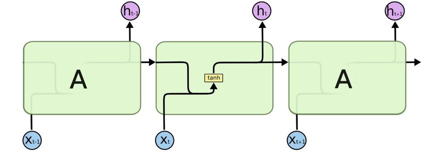
Table of Contents
1. Introduction ...................................................................................................... 4
 1.1 Background ............................................................................................... 4
 1.2 Relevance .................................................................................................. 5
 1.3 Purpose ...................................................................................................... 5
 1.4 Scientific novelty ....................................................................................... 6
 1.5 Structure of the research ............................................................................ 6
2. Overview of pollution level modeling ............................................................. 7
 2.1 Deterministic methods ............................................................................... 7
 2.2 Non-deterministic methods ....................................................................... 9
3. Machine learning algorithms ......................................................................... 13
 3.1 Time series models .................................................................................. 13
 3.1.1 Univariate analysis ........................................................................... 13
 3.1.2 Multivariate analysis ........................................................................ 15
 3.2 Classical machine learning methods ....................................................... 15
 3.2.1 Regularized linear regression ........................................................... 16
 3.2.2 Support Vector Regression .............................................................. 16
 3.2.3 Decision tree..................................................................................... 17
 3.3 Ensemble learning methods..................................................................... 19
 3.3.1 Horizontal ensemble......................................................................... 19
 3.3.2 Vertical ensemble ............................................................................. 19
 3.4 Artificial Neural Networks ...................................................................... 20
 3.4.1 Multilayer perceptron ....................................................................... 20
 3.4.2 LSTM neural network ...................................................................... 21
 3.4.3 CNN neural network ........................................................................ 23
4. Modeling pollution level ................................................................................ 25
 4.1 Data ......................................................................................................... 25
 4.2 Methodology of modeling ....................................................................... 27
 4.3 Modeling ................................................................................................. 29
5. Discussion and Conclusion ............................................................................ 35
6. References ...................................................................................................... 36
7. Appendix ........................................................................................................ 40

 3

1. Introduction
1.1 Background
The global population that is currently around 7.8 billion has increased by 100%
the last 40 years and is estimated to increase by 50% during the period of the next
40 years reaching 9 billion by 2037 (Ahmadov, 2016). Most of the growth occurs
in urban areas of the developing parts of the world and has as a result the overuse
and shortage of natural resources, deforestation, climate change and especially
environmental pollution (Ritter et al., 1992).

According to the World Health Organization (WHO) air pollution is the main
environmental health issue that affects all regions of the world and has caused 4.2
million premature deaths all over the world during 2016. However, the inhabitants
of low-income cities are the most impacted ones. This fact is supported by the
latest air quality database which indicates that 97% of cities in low- and middle-
income countries with more than 100,000 residents do not respond to WHO air
quality principles (guidelines) (Rybarczyk & Zalakeviciute, 2018).

The outdoor air pollution affects large cities as well as rural areas and is caused by
multiple factors like industry and energy supply, waste management, transport,
dust, agricultural practices and household energy (Zalakeviciute et al., 2018).
Pollutants that have been proved as being the most dangerous for public health
concern include particulate matter (PM), ozone (O3), nitrogen dioxide (NO2) and
Sulphur dioxide (SO2). The most registered health risks are related to particulate
matter of less than 10 and 2.5 microns in diameter (PM10 and PM2.5). PM is
capable of penetrating deep into lung passageways and entering the bloodstream
causing cardiovascular, cerebrovascular and respiratory impacts. Additional
serious health issues that induced by air pollution are according to WHO heart
disease, stroke, chronic obstructive pulmonary disease, lung cancer (WHO, 2014).

It is not only the human health that is critically impacted by the air pollutants but
also the earth’s climate and ecosystems globally (WHO, 2014). Air quality can
impact climate change and climate change can respectively impact air quality.
Emissions of pollutants into the air can have as a result the climate changes. Ozone

 4

in the atmosphere warms the climate, while different components of particulate
matter (PM) can have either warming or cooling effects on the climate. On the
other hand, changes in climate can affect the local air quality. Atmospheric
warming related to climate change, potentially increases ground-level ozone in
many regions and due to this fact, there may be challenging to comply with the
ozone standards in the future. The impact of climate change on other air pollutants
is still uncertain but many studies are in progress to manage this uncertainty
(Brunelli et al., 2007).

1.2 Relevance
Due to the information mentioned above, it is indisputable fact that the prediction
and the monitoring of the air quality is of the utmost importance both for human
health and climate progress. The present comparative study between Weather
Research and Forecast Chemistry model (WRF-Chem) and machine learning
(statistical method) air quality prediction (Carnevale et al., 2009), will be based on
the available data from the meteorological station of the Cuenca city in Ecuador.

1.3 Purpose
The purpose of this study is to compare the accuracy of the prediction between a
WRF-Chem model and a Statistical Model built from machine learning algorithms
and investigate which of the two methods is better in the forecasting of the
concentration of fine particulate matter (PM2.5) in an urban complex terrain as
well as the meteorological conditions.

In order to reach our goal, we need to determine which machine learning
algorithms might be used predict air quality, build those models and conduct a
final comparison regarding accuracy, complexity and time costs

Our methodology is to compare benchmark with methods developed throughout
the process. We use WRF-Chem’s prediction error as a benchmark to compare
with results of different statistical methods and machine learning algorithms.

 5

1.4 Scientific novelty
Current studies show that traditional deterministic models tend to struggle to
capture the non-linear relationship between the concentration of air pollutants and
their sources of emission and dispersion (Shimadera et al., 2016). To tackle such a
limitation, very promising approach is to use statistical models based on machine
learning techniques (Chen et al., 2017). We try broad variety of different statistical
approaches to overcome the issue, including ensemble learning and sequence-to-
sequence neural network models. Related literature demonstrates usage of machine
learning models to predict air pollution level for the next day. We will create and
evaluate a module allowing for multistep prediction.

1.5 Structure of the research
The paper consists of introduction, three chapters, discussion, conclusion,
reference list and appendix. First chapter is an overview of best practices used in
the field to predict air pollution. We will compare deterministic and non-
deterministic approach and discuss advantages of either of both. Second chapter
explains statistical methods used in the study. We also discuss their advantages,
disadvantages and suitability for the paper’s goal. Third chapter contains empirical
part of the present research. It tells about data used and its preprocessing. Then we
built selected machine learning algorithms and test them against the benchmark.

 6

2. Overview of pollution level modeling
In the related literature forecasting of the pollution level usually is performed
using one of two approaches: deterministic and statistical. This logically leads to
the structure of present chapter. In the deterministic approach prediction is made
based on field-specific knowledge about data, e.g. laws of physics and chemistry.
In the non-deterministic approach, researcher uses statistical models and
algorithms to extract rule from the data with no or little prior knowledge
(Armstrong, 2002).

2.1 Deterministic methods
Deterministic models are usually represented by systems of models that work
together to simulate emission, transport, diffusion, transformation, and removal of
air pollutants. Those models are namely meteorological models, emissions models,
air quality models. Pollutant concentration forecast can be performed using simple
one-dimensional air quality models, but three-dimensional models are used to
simulate complex interactions of physical and chemical processes (U.S.
Environmental Protection Agency, 2003).

One of the most widely used meteorological models is the Penn State/NCAR
Mesoscale Model version 5 - MM5. Which is a regional mesoscale model used for
weather forecasting and climate projections maintained by Penn State University
(Grell et al., 1994). Another prime example is the Regional Atmospheric Modeling
System – RAMS which is a comprehensive mesoscale meteorological modeling
system (Pielke et al., 1992).

In the process of emission modeling estimated emission with the spatial, temporal
and chemical resolution are used to model air quality (Pielke et al., 1992). Data on
emission includes mobile sources, stationary sources, area sources and natural
sources. Most used emission modeling systems are Emission Processing System
(EPS 2.0) (U.S. Environmental Protection Agency, 1992), Emissions Modeling
System (EMS-95 – EMS-2002) (Bruckman, 1993) and Sparse Matrix Operator
Kernel Emissions (SMOKE) modeling system (Coats, 1996).

 7

There are two types of three-dimensional models: Lagrangian and Eulerian;
depending on the method used to simulate the time-varying distribution of
pollution concentrations. Lagrangian models trace individual air parcels of air over
time using meteorological data to transport and diffuse the pollutants that is why
they are also called trajectory models. However, the fact the model traces each
individual parcel of air makes it computationally inefficient if interaction of a large
number of individual sources when nonlinear chemistry is involved, and these
models have limited usefulness in forecasting secondary pollutants (Pielke et al.,
1992).

Eulerian models use a grid of cell (vertical and horizontal) where the chemical
transformation equations are solved in each cell and pollutants are exchanged
between cells. These models can produce three-dimensional concentration fields
for several pollutants but require significant computational power. Typically, the
computational requirements are reduced using nested grids, with a coarse grid used
over rural areas and a finer grid used over urban areas where concentration
gradients tend to be more pronounced (Pielke et al., 1992).

The Hybrid Single-Particle Lagrangian Integrated Trajectories with a generalized
nonlinear Chemistry Module (HY-SPLIT CheM) model is an example of a
Lagrangian model used to forecast air quality on a regional scale (Stein et al.,
2000). However, these models struggle to works with big number of emission
sources, so Eulerian models are used more often for the urban scale. Popular
Eulerian models include multiscale Air Quality Simulation Platform (MAQSIP)
(Odman & Ingram, 1996), SARMAP Air Quality Model (SAQM) (Chang et al.,
1996) and Urban Airshed Model with Aerosols (UAM-AERO) (Lurmann, 2000).

Very popular deterministic model is Weather Research and Forecasting with
Chemistry (WRF-Chem V3.2) (WRF, 2017). WRF is a 3-D last-generation non-
hydrostatic model used for meteorological forecasting and weather research. It is a
fully compressible model that solves the equations of atmospheric motion, with
applicability to global, mesoscale, regional and local scales. WRF also has the
configuration WRF-Chem for modeling the interactions between meteorology and
transport of pollutants.

 8

It is not rare that deterministic models are developed for some specific regions.
Finardi et al. developed deterministic module to forecast air quality in Torino city
(Finardi et al., 2008). Modeling system is based on prognostic downscaling of
weather forecasts and on multi-scale chemical transport model simulation in order
to describe atmospheric circulation in a complex topographic environment,
space\time variation of emissions and pollutant import from neighboring regions.

2.2 Non-deterministic methods
Quite often authors use broad variety of machine learning models and conduct
comparative analysis of the results. Saniya et al. use level of precipitation, wind
speed and wind direction to predict concentration of PM2.5. Authors use Linear
Regression, Multilayer Perceptron, Support Vector Machine and M5P model
Trees. Collaborative filtering algorithm has played a major role by making
automatic and accurate predictions based on previous trends of pollutant levels and
database in the server (Saniya et al., 2018).

Sayegh et al. also employ a number of machine learning models including Linear
Regression, Quantile Regression, Generalized Additive model and Boosted
Decision Trees model to compare the performance to predict PM10.
Meteorological factors including wind speed, wind direction, temperature,
humidity and chemical species including CO, NOx, SO2, PM10 value for the
previous time step data for one year from Makkah, Saudi Arabia are used. Quantile
Linear Regression shows better results due to the fact that covariants are affecting
quantiles heterogeneously which is lost in the central rendency prediction
framework (linear regression) (Sayegh et al., 2014).

Singh et al. in their paper identity sources of pollution and forecast the air
pollution level using variuos machine learnig models: Hybrid Model with
Principal Components Analysis, Support Vector Machine and ensemlbe learning
models – Random Forest and Boosted Desicion Tree. Authors use five years of
pollution level and meteorological variables data for Lucknow, India. Models are
used ro predict Air Quality Index and Combined AQI. They also research
importance of predictors and their influence on the forecast. Boosted Decision

 9

Tree in that paper shows the best result closely followed by Random Forest (Singh
et al., 2013).

Philibert et al. use Random Forest and Linear and Nonlinear Regression to predict
N2O emission level. They use data on environmental and crop variables including
fertilization, type of crop, experiment duration, country, etc. on the global scale.
Authors use variabe selection to rank variables by importance and include only the
most informative ones, which results in the increased accuracy. Random Forest
model shows the vest result (Philibert et al., 2013).

In the paper by Nieto et al. authors aim to predict various pollutants’ level
including NO2, SO2 and PM10 in Oviedo, Spain based on a number of
meteorological factors. They use Multivariate Adaptive Regression Splines and
Multilayer Perceptron model on three years of historical data (Nieto et al., 2015).
Kleine Deters et al. use six years of meteorological data including wind speed and
precipitation for Quito, Ecuador to identify the meteorology effects on PM2.5.
They use Linear Regression as this statistical method offers excellent
interpretability and allows for easy analysis of statistical significence of
independent variables (Kleine et al., 2017).

Carnevale et al. aim to estimate the relationship between PM10 emission and
pollutants from the Air Quality Index for Lombard region, Italy using hourly data
on SO2, Nox, CO, PM10 and NH3 for a year. The Dijkstra algorithm is deployed
in the large-scale data processing system. Model’s performance then was
comapaired against deterministic model simulation. Performance of the model is
close to the Transport Chemical Aerosol Model which is computationally much
more expensive (Carnevale et al., 2018).

Suárez Sánchez et al. investigate the dependence between primary and secondary
pollutants and most significant contributors to air pollution level. Data include
three years of observations of NOx, CO, SO2, O3 and PM10 in Aviles, Spain.
Authors use various Support Vector Machine kernels including radial, linear,
quadratic, Pearson VII Universal Kernels and Multilayer Perceptron Model to
predict NOx, CO, SO2, O3, and PM10. Aviles, Spain. Best quality was achieved
using Pearson VII Universal Kernel (Suárez et al., 2011).

 10

Liu et al. also use SVM to predict Air Quality Index training models on two years
of observations from three cities in China (Beijing, Tianjin, and Shijiazhuang).
Data includes AQI values, various pollutants’ concentrations (PM2.5, PM10, SO2,
CO, NO2, and O3), meteorological factors (temperature, wind direction and
velocity), and weather descriptions (ex. cloudy/sunny, or rainy/snowy, etc.). The
model performance was significantly improved after including the surrounding
cities’ air quality levels (Liu et al., 2017).

Another paper use SVM to forecast pollutants’ (NO2, SO2, O3, SPM) levels from
historical and meteorological data from Macau, China by Vong et al. Authors use
three years to train the model and ine year to evaluate the performance. The
Pearson correlation is used to identify the best predictors for each pollutant and
different kernels are used to test which of the predictors or models get the best
results. They also use Pearson correlation as a metric to determine optimal number
of days for forecsting. They achieve a good fit and conclude that SVM’s
performance crucially depends on the choice of kernel (Vong et al., 2012).

Study by Zhan et al. uses Random Forest model to build a spatiotemporal model to
predict O3 concentration across China. They use RF with 500 estimators (decision
trees). Dataset includes one year of observations for meteorology variables,
planetary boundary height, elevation, anthropogenic emission inventory, land use,
vegetation index, road density, population density, and time from 1601 stations
located all across China. Performance of the model is evaluated against Chemical
Transport models’ simulations using RMSE and R squared as metrics. Machine
learning models show better accuracy at the same time being less consumong in
terms of computationsl resourses. They also conclued that accuracy of prediction
relies heavily on the quality of coverage by the monitoring network (Zhan et al.,
2018).

Martínez-España et al. aim to find the most robust machine learning algorithms to
preserve accuracy in case of O3 monitoring failure. Authors use Decision Tree, k-
Nearest neighbours model, Bagging model, Random Cometee and Random Forest.
They compare performance of selected models and then use hierarhical clustering
to determine optimal number of models to predict the O3 level in the region of
Murcia, Spain. Random Forest slightly outperforms the other models. The best
 11

predictors turns out to be NOx, temperature, wind direction, wind speed, relative
humidity, SO2, NO, and PM10. They also conclude that two models are enough
for chosen data (Martínez-España et al., 2018).

In the paper by Bougoudis et al. authors identify the conditions under which high
pollution emerges. They use Hybrid system based on the combination of
clustering, Artificial Neural Networks, Random Forest and fuzzy logic. Twelve
years of hourly observations of CO, NO, NO2, SO2, temperature, relative
humidity, pressure, solar radiation, wind speed and direction from Athens, Greece
are used. The optimization of the modeling performance is done with Mamdani
rule-based fuzzy inference system that exploits relations between the parameters
affecting air quality. Specifically, self-organizing maps are used to perform dataset
re-sampling, then ensembles of feedforward artificial neural networks and random
forests are trained to clustered data vectors (Athanasopoulos et al., 2017).

Elangasinghe et al. is one of the earlier papers using neural networks to predict
concentration of NO2. They use genetic algorithm to optimize inputs for the neural
network. Variables set includes wind speed, wind direction, solar radiation,
temperature, relative humidity and time features accounting for hour, day and
month (Elangasinghe et al., 2014).

Gardner and Dorling concluded that neural networks outperform other linear
statistical methods regarding non-linear dependency (Gardner & Dorling, 1999).
Perez conducted comparison between persistence method, linear regression and
neural network using data from Santiago, Chile. He concluded that the best error
on the hourly prediction of pollution level was obtained using neural networks
(Pérez et al., 2000). Brunelli et all used recurrent neural networks to predict
concentration of various pollutants for two days ahead using meteorological data
(Brunelli et al., 2015).

Some authors have been improving neural networks’ accuracy using other
methods. Grivas et al. uses a neural network capable of combining meteorological
and time-scale input to predict hourly pollution level over the Greater Athens Area
using data collected in 2001-2002. Their model greatly outperformed linear
regression used for comparison (Finardi et al., 2008).

 12

3.Machine learning algorithms
Machine learning methods gradually infiltrate time series analysis and pollution
level modeling. However, properly configurated, they hold powerful potential. In
this chapter, we are going to do a quick recap of the time series models and discuss
machine learning models.

3.1 Time series models
For the univariate time series analysis, we are going to use two models: SARIMA
and Holt-Winters Exponential Smoothing. For the multivariate time series
analysis, we are going to use vector autoregressive model (VAR).

3.1.1 Univariate analysis

The autoregressive integrated moving average (ARIMA) is a classical time series
model designed to analyze and forecast time series data (Zhang, 2001). It is a
generalization over ARMA model in which data is supposed to be non-stationary.
Equation 1 shows ARMA model with autoregressive component of order and
moving average component of order .

 = 0 + 1 −1 + ⋯ + − + + 1 −1 + ⋯ + − (1)

To use ARIMA model we need to be sure that our data is stationary, meaning that
it has a constant mean and variance regardless of time step. ARIMA models
assures stationarity using differencing, as difference (on practice has a high chance
of being stationary. Equation 2 shows differencing process.

 ′ = − −1 (2)

In case of seasonal data, we apply seasonal differencing showed in the equation 3,
in which depicts assumed seasonality:

 ′′ = ′ − − 
 ′ (3)

 13

Once we have treated non-stationarity and seasonality in our data using
differencing, we can write high-level representation of SARIMA model shown in
equation 4.
 ( , , ) ( , , , ) (4)

 • is an order of autoregressive component (AR)
 • is an order of non-seasonal differencing
 • is an order of moving average component (MA)
 • is an order of seasonal AR
 • is an order of seasonal differencing
 • is an order of seasonal MA
 • is a number of periods in the season

Holt-Winters Exponential Smoothing is an extension of Holt’s method to capture
seasonality (Winters, 1960). Model consists of forecast equation (equation 5) and
three smoothing equations: for the level (equation 6), for the trend (equation
7), for the seasonal component (equation 8). Corresponding smoothing
parameters , and are estimated using error minimization. Parameter 
accounts for the frequency of seasonality.

 ̂ +ℎ| = + ℎ + +ℎ− ( +1) (5)

 = ( − − ) + (1 − )( −1 + −1 ) (6)

 = ( − −1 ) + (1 − ) −1 (7)

 = ( − −1 ) + (1 − ) −1 (8)

Method has two variations: additive is preferred when the seasonal variations are
roughly constant throughout the series, while the multiplicative method is
preferred when the seasonal variations are changing proportional to the level of the
series. Due to the nature of our data, we use the additive model.

 14

3.1.2 Multivariate analysis

Vector autoregressive model is a generalization of the univariate autoregressive
model which allows for forecasting of a vector of time series (Athanasopoulos,
2017). All the variables affect each other and are treated equally. For example,
three-dimensional VAR is described by system of equations shown in equation 9.

 1, = 1 + 11,1 1, −1 + 12,1 2, −1 + 13,1 3, −1 + 1, 
 { 2, = 2 + 21,1 1, −1 + 22,1 2, −1 + 23,1 3, −1 + 2, (9)
 3, = 3 + 31,1 1, −1 + 32,1 2, −1 + 33,1 3, −1 + 3, 

Where 1, , 2, and 3, are white noise processes that may be contemporaneously
correlated.

3.2 Classical machine learning methods
The most widely used machine learning is a classical linear regression, using least
square method to get coefficients’ estimations. Linear regression model can be
written as an equation 10, where is a target variable; is an explanatory
variable; is weight for explanatory variable; is an error between predicted and
observed values.
 = 0 + 1 1 + 2 2 + ⋯ + + (10)

Vector of weights is found using minimization problem shown in equation 11:

 1 2
 ( ∑ ( ( ) − ) ) (11)
 
 =1

Whether our coefficients are correct and well representing reality depends on the
compliance to the set of assumptions: linear dependency between target variable
and predictors; target variable should be normally distributed; homoskedasticity
means that variance of error is assumed to be constant throughout data; each
observations supposed to be independent; absent of multicollinearity mean that our
variables are independent with each other.

 15

3.2.1 Regularized linear regression

In the era of big data, the researcher may find himself in a situation where the
number of variables exceeds the number of observations, in the case of the
classical least-squares method, this leads to overfitting and zero predictive ability.
The potential multicollinearity of variables and the need to get rid of a number of
these in the analysis process are also big problems (Zou & Hastie, 2005).

In order to combat these problems, models of normalized least squares were
presented. The two most popular models - ridge and lasso - are very similar and
differ only in the specification of the penalty component (normalization form).
Let's take a closer look at the lasso model.

Lasso is an autonomous and convenient way to introduce sparseness into a linear
regression model. The lasso abbreviation stands for “the operator of the smallest
absolute shrinkage and selection” and, when applied to the linear regression
model, performs the selection of features and regularization of the weights of the
selected objects. Lasso adds a penalty component to the OLS minimization
problem as shown in equation 12.

 1 2
 ( ∑ ( ( ) − ) + ‖ ‖ ) (12)
 
 =1

Component || || 1 is the 1 norm of the variable vector, which leads to a penalty
for large weights. Since the 1 norm is used, many weights get a score of 0 (in the
case of the ridge model, the 2 norm is used, which leads to the fact that the
weights can be arbitrarily small, but not zero) and the rest are reduced. The lambda
parameter controls the degree of regularizing effect and is usually tuned by cross-
validation. When the lambda is large, many weights become equal to 0.

3.2.2 Support Vector Regression

Support vector machine (SVM) is a classical machine learning algorithm often
used as a benchmark to measure more complex models’ efficiency due to its speed
and accuracy (Basak et al., 2007).

 16

The basic idea of SVM is to find a separating hyperplane separating classes (in the
case of classification). In the case of regression analysis, the task is similar in
appearance to constructing linear regression (minimizing the error), with the
difference that in the case of the support vector model, the task is to conclude the
error within a certain threshold. Optimization problem is formulated as system of
equations shown in equation 13.

 1
 ‖ ‖2 + ∑(ξ + ξ∗ ) → 
 2
 =1
 (13)
 − ⟨ , ⟩ − ≤ + ξ 
 ⟨ , ⟩ + − ≤ + ξ ∗
 { ξ , ξ∗ ≥ 0

 where С – penalty for the estimation error;
 – estimation error;
 ξ , ξ ∗ – slack variables;
 – vector of weights;
 – vector of independent variables;
 – dependent variable.

In the case when the set of objects is linearly inseparable, it is necessary to move
from the original space to a space of higher dimension, in which the classes are
linearly separable. Examples of the most popular mappings:

 • Linear: ( , ) = ;
 
 • Polynomial: ( , ) = (1 + ) ;
 2
 ‖ − ‖
 • Gaussian: ( , ) = exp (− );
 2 2

 • Sigmoid: ( , ) = tanh( 0 + 1 ).

3.2.3 Decision tree

Decision trees are a family of algorithms that play an important role in machine
learning (Thomas, 2000). Due to the simple method of generating decision trees,
decision tree learning is quick and easy compared to more complex algorithms
(Cruz & Wishart, 2006). The tree structure consists of branches of several edges

 17

connected by internal vertices and leaves at the end of each branch. Each leaf at
the end makes a prediction.

For partitioning, the simplest condition is used, which checks whether the value of
some attribute lies to the left of the specified threshold : [ ≤ ]. Let the set
 objects from the training set be at the vertex . The parameters in the
condition will be chosen to minimize the error criterion (e. g. in classification
problem Gini impurity index can be used; regression problem can use mean
absolute error).

The parameters and can be selected by enumeration. There are a finite number
of features, and of all the possible values of the threshold , we can consider only
those for which various partitions are obtained. After the parameters have been
selected, the set of objects from the training set is divided into two subsets,
each of which corresponds to its child vertex.

Procedures is repeated until the desired accuracy or stopping criteria is met. The
accuracy of the decisive trees increases with their depth. The deeper the tree, the
more complex, non-monotonous dependencies it can catch. However, increasing
depth leads to unwanted consequences:

 • Loss of interpretability;

 • Severe overfitting, as tree deep enough can reach 100% accuracy on train
 data while being unable to perform good enough on test data.

The main way to combat retraining is to normalize and select model
hyperparameters that, on the one hand, will show good results on training data, and,
on the other hand, will be able to produce greater accuracy of predictions on
validation data.

The main hyperparameters used to normalize decision trees are the maximum
depth of the tree (i.e., the maximum number of divisions down the tree), the
minimum number of observations at the terminal vertex (i.e. the minimum number
of observations in the tree leaf needed to happen division).

 18

3.3 Ensemble learning methods
Another way to solve the overfitting problem is ensemble learning. The idea of
ensemble is to average the predictions of several weak predictors and combine
them into one model, which will have high predictive ability (high accuracy).
After this, the prediction is conducted by combining the results of all weak
predictors, for classification, the simple majority voting rule can be used, for
regression – averaging.

In the modeling process, it is important to obtain the most different (minimally
correlating) weak predictors among themselves. The main methods used to achieve
this goal are bootstrap and random selection of a limited number of variables for
each weak predictor. A bootstrap consists of selecting random observations from a
common sample to train each weak predictor. With a bootstrap with repetition, the
same observation can enter the model training dataset several times.

3.3.1 Horizontal ensemble

During the horizontal ensemble, we train several weak predictors independently of
each other. One of the most popular examples of parallel ensemble is a random
forest (RF). A random forest is an ensemble of decision trees, each operating
independently, making a prediction as to where an example data entry belongs.
The forest aggregates the results and chooses the strongest prediction (Andy &
Matthew, 2002). The random forest algorithm, can be described as follows:

 1. We draw bootstrap samples from the dataset;
 2. For each sample we create an unpruned decision tree based on features in
 the dataset;
 3. We get predictions from trees which are then averaged by voting
 (classification) or average (regression).

3.3.2 Vertical ensemble

During vertical ensembling, we train several weak learners consequently. In
general, sequential ensemble allows to obtain higher accuracy of predictions than
parallel trained models. However, that model loses in terms of speed, as due to the
fact of sequential fit it is impossible to parallel computation. This model is also

 19

even more prone to overfitting, which requires use of regularization. One of the
most popular algorithms, gradient boosting, can be described as follows:

 1. We get the initial model’s error (e. g. decision tree or linear regression):
 1 = − ̂1 ;
 2. Estimate error for the model in which error from the first step is used as a
 dependent variable: ̂
 1;

 3. Sum obtained prediction with the original: ̂2 = ̂1 + ̂
 1;

 4. Get the new error: 2 = − ̂2 ;
 5. Repeat steps 2-4 until we overfit or until model’s error become constant.

Most popular algorithms are Gradient Bosting Machine (GBM) described before
and Extreme Gradient Boosting (XGBoost) using shortcuts in the conventional
algorithm to achieve faster computational speed at the expense of potential
accuracy loss.

3.4 Artificial Neural Networks
3.4.1 Multilayer perceptron

The simplest version of neural network is called multilayer feed-forward
perceptron. It is simply defined as an input layer, an output layer, and several
hidden layers. Each layer consists of multiple artificial neurons, which are tasked
with feeding forward data to the next layer (Svozil et al., 1997). Figure 1
represents simple neural network schematically.

Figure 1. Example of a feed-forward neural network with one hidden layer (Svozil et al., 1997)

 20

Each node of the network consists of an artificial neuron, a mathematical model
intended to emulate the role of a neuron in a physical brain. Each neuron consists
of a set of inputs, some type of activation or transfer function, and an output
(Svozil et al., 1997). The inputs multiplied by weights and added to biases are
passed to the further layers (forward propagation). Example of artificial neuron is
shown in figure 2.

Figure 2. Artificial neuron schema (Svozil et al., 1997)

There are several activation functions in practice, the most popular is sigmoid.
Process of training of the neural network can be describe by the following steps:

 1. Network receives training data as its input which through feed-forward
 propagation becomes the set of outputs;
 2. Error is calculated (usually for the regression problem it is mean square
 error;
 3. Partial derivatives of the loss function are calculated with respect to the
 model’s parameters;
 4. Model parameters are tuned with respect to mentioned derivatives
 (backpropagation).

3.4.2 LSTM neural network

Classical neural network is poorly suitable for the time series prediction as they are
analyzing each datapoint separately, not being able to bear information over time
or any other sequence (e. g. language). This problem gets resolved by Recurrent

 21

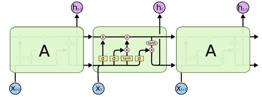
neural network (RNN), as they use previous state as another input. Figure 3
represents simple recurrent neural network schematically.

Figure 3. Reccurent neural network (3 units) (Olah)

However, if the input sequence is long, RNN gives more attention to the later
datapoints, while memory about old ones vanishes. This problem is overcame
using Long Short-Term Memory neural networks (LSTM) as they are able to learn
long-term dependencies (Olah).

In order to have such ability, LSTM has three layers inside of a unit. The most
important idea behind the model is a cell state, information ‘conveyer’ running
through the entire network. Information goes to cell state through three gates.
Forget gate decides what part of the information needs to be withdrawn from the
cell state. Input gate decides which part of information is going to be passed to
enter the cell state. Output gate decides which part of data is going to be outputted.
Example of LSTM network’s unit is shown in figure 4.

Figure 4. LSTM neural network (3 units) (Olah)

 22

LSTM can be used to map sequence to scalar or vector, to a single or multiple time
steps. WE train itusing classical backpropagation taking derivatives of the loss
fucntion once comparison of factual and expected output are obtained Those
derivative are used as weights to update parameters inside neural network’s layers.

3.4.3 CNN neural network

Convolutional neural network is the most popular as image processing models (or
at least the most popular building block). Key idea behind CNN is using a set of
filters to gradually learn mode and more complex features (Stewart). Close
analogy would a flashlight gliding over an image. Using this “flashlight” with
convolutional layers we significantly reduce number of trainable parameters.
Example of convolutional layer is given in figure 5.

Figure 5. The convolution operation (Stewart)

Latter is a major improvement over classical neural network, as it uses one input
per pixel, and moderate resolution picture processing results in hundreds of
thousands of trainable parameters. So, at first CNN learns simple shapes or even
shades, then gradually it learns more and more complicated features until by the
last layer is can recognize a nose on the picture and even tell which animal it
belongs to.

 23

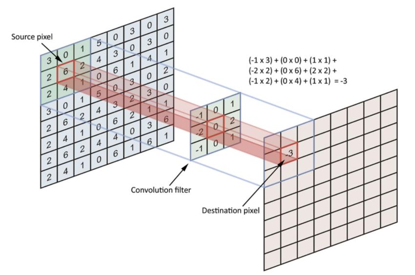
Figure 6. Simple CNN example (Stewart)

Figure 6 represents simple CNN architecture. CNN can also be applied to time
series data, as we glide with a 1D filter over the sequence of observations mapping
it to the output which can be in scalar or vector form while latter can be
represented bya single or multiple time steps. As any other neural network, CNN
is trained using backpropagation.

 24

4. Modeling pollution level
This is the empirical part of the present research. We start by describing data used
and preprocessing steps taken. We also discuss metric chosen for model
comparison; feature engineering required to account for time nature of our data. In
the end we build models and conduct comparison with the benchmark. We use
programming language Python 3.5 for our analysis, code for modeling is available
in the appendix. For time series analysis we use statsmodels library. Machine
learning models are built using sklearn library. To build neural networks we use
Keras library operating on top of Tensorflow library.

4.1 Data
We are using 5 years of hourly data on chemical (PM2.5) and meteorological
(temperature, relative humidity, solar radiation, wind speed and wind direction)
variables collected from a monitoring station located in Cuenca, Ecuador. As
WRF-Chem provides daily observations, we down sample data to daily
observation using mean as aggregation function.

Unfortunately, our data has a lot of missing observations. Even worse, dates for
which observations are missing are not consistent over variables. E.g., wind speed
and wind direction don’t have observations for the majority of 2016, while
temperature is missing for the second half of 2015 and 2 months of 2017. Having
said that, we cannot just drop missing observations, as this result in the reduction
of our dataset from 1518 to ~350 observations. Hence, we use interpolation.

For some variables (e.g. temperature) best interpolation technique proved to be
spline of order 5, others (e.g. solar radiation) were best approximated by simple
linear interpolation. Interpolation was chosen by the criteria of the best fit for
existing data. Possible shortcomings of that approach are discussed in the
discussion section of the present paper.

Prior to modeling we need to clean our data from outliers. Some data can be just
false (for example, negative pollution level), some days show extremely high value
of some variables, which can adversely affect the training process and result in a
loss of accuracy.

 25

To detect outliers, we are going to use interquartile range. The interquartile range
( ) is a measure of statistical dispersion and is calculated as the difference
between the 75 ℎ and 25 ℎ percentiles (percentile is a measure indicating the
value below which a given percentage of observations falls). It is represented by
the formula = 3 − 1. After calculating for each variable, we limit
the variable in the interval between 1 – 1.5 and 3 + 1.5 . Table 1
shows statistical description of data.

Table 1. Statistical description of data

 pm temp hum sol wind_dir vel_ms

 count 1583 1583 1583 1583 1583 1583

 mean 9.15 15.25 64.40 191.89 161.79 1.72

 std 3.81 1.12 8.06 70.96 50.66 0.34

 min 0.00 11.30 25.59 0.00 11.08 0.46

 25% 6.57 14.42 59.45 130.56 129.70 1.60

 50% 8.99 15.23 64.67 186.47 157.12 1.64

 75% 11.51 15.98 69.24 244.39 189.01 1.92

 max 21.40 19.11 91.12 472.04 307.62 3.02

Some statistical models can be sensitive to difference in magnitude of variables.
For example. Linear regression performs better if all the variables are scaled (or
normalized), tree-based algorithms in general are less sensitive, for neural
networks normalization is a must, as it allows for faster convergence and better
accuracy (Ali & Faraj, 2014). We are going to use a wide range of machine
learning models. So, it is better to perform some transformation on our data.

We are using min max normalization to assure that all the variables have the same
magnitude (contained within 0 and 1). Normalization is performed as shown in
equation 14.

 26

 − 
 = (14)
 − 

It is worth mentioning that data is quite erratic without clear trend and/or
seasonality. This further nudge us to use machine learning as those models in
general are more suitable to model complicated non-linear dependencies. Figure 7
shows erratic nature of pollution level time series.

 1

 0.9

 0.8

 0.7
 Level of PM2.5

 0.6

 0.5

 0.4

 0.3

 0.2

 0.1

 0
 2014-09-01 2015-09-01 2016-09-01 2017-09-01 2018-09-01

Figure 7. Pollution level time series

4.2 Methodology of modeling
Evaluation metric

To evaluate models’ results we are using mean absolute error (MAE) metric, used
a lot assessing regression problem. I have chosen absolute over root squared mean
error as our data is erratic and thereby, I do not want to inflict additional
punishment for outliers. Formula to calculate MAE is shown in equation 15.

 1 
 = ∑ | − ̂ | (15)
 =1

Where is an observed value of dependent variable, ̂ is a predicted one and is
the size of testing sample.

 27

Time features

For time series modeling we just use our six time series, but to use machine
learning algorithms we need to add time features explicitly. I add ℎ ,
day_of_week and week_of_year features (whole numbers) to account for weekly
and annual trend in data.

Then, for each variable I add values at 6am, 1pm and 3pm as those hours provide u
with the most representative concentrations of pollutants over the day. 6am is the
beginning of the morning peak, 1pm corresponds to the midday baseline and 3pm
is the beginning of evening peak. Then, for all the variables excluding ℎ,
 _ _ and _ _ I add lagged values up to 5th lag (e.g. 2nd lag is a
value observed two days ago). This way we account for time nature of the data.

Walk forward validation

In order to make our evaluation robust, we use cross-validation. Using 5-n cross-
validation we split dataset into 5 parts. Then we train our model on the first four of
them. We use last part of our dataset, not used in the training process, for
validation. Once we get the MAE, we save it and repeat the process using first,
second, third and fifth parts for training and the fourth one for evaluation, getting
another MAE (the process is repeated 5 times). This way we guarantee that our
model has been evaluated on all the available data.

Unfortunately, it is not feasible in case of time series models. We could use cross-
validation for the machine learning models non-depended on the sequential
structure. However, for time series models time structure is a requirement. So, we
need better approach for evaluation, applicable both to time series models and to
machine learning models.

We are going to use walk forward cross-validation. This approach requires two
sliding windows for training and test set. Schematically approach is depicted in
figure 8. For each test set we will calculate a separate MAE and then take the
average of them. Sliding over dataset allows for robustness in evaluation in
training.

 28

Figure 8. 4-n walk forward cross-validation (Moudiki, 2020)

4.3 Modeling
Biggest problem of our data is the fact that we only have WRF-Chem prediction
for September 2014. At the same time, our dataset stretches from 2014 to 2018.
We overcome this issue reversing our data, so order is preserved, but reversed. At
the same time, models fit and tuned to predict specifically September 2014 have a
chance to lack robustness. So, at first, we evaluate our models using walk forward
cross-validation with training window of two years. Then, we take best models and
compare forecast for September 2014 to the benchmark.

Time series analysis models

Prior to build our time series models, we conduct Augmented Dickey-Fuller with
constant and trend test for each sequence. Null hypothesis for the test states that
series are not stationary. Results are shown in table 3.

Table 3. Augmented Dickey-Fuller test results

Time series p-value conclusion
pollution level 8.8306e-06 series is stationary
temperature 0.0002 series is stationary
humidity 0.0 series is stationary
solar radiance 0.0306 series is stationary
wind speed 1.1e-09 series is stationary
wind direction 2.441e-06 series is stationary

 29

As we can see, all our series are stationary, and we can proceed. We are using test
window of 30 observations with 5-n walk forward cross-validation. For univariate
analysis we use SARIMA model, as changing its parameters allows us to test
broad scope – from AR to SARIMA. For multivariate analysis we use classical
VAR model. Best configuration was chosen based on best Akaike information
criteria after simple iteration over different order of lags. Results are shown in
table 4.

Table 4. Time series models results

Model MAE
SARIMA (2,0,1) (0,0,0,12) 0.1475
VAR (9) 0.1237
Holt-Winters 0.1368

Vector autoregressive model of order 9 shows the best quality of fit with the
average MAE of 0.12.

LSTM models

Next, we fit neural network models with 5-n walk forward cross-validation. We
start with long short-term memory neural networks. First, we try different
configurations to predict pollution level one day ahead. Single channel model uses
only historical data on pollution level. Multichannel models use historical data on
all the available time series (pollution level, humidity, solar radiance, temperature,
wind direction and wind speed). Multichannel output models allow us to predict
not only the target variable but all the series, like VAR model. Our architecture
consists of LSTM layers with 50 units followed by fully connected layer. Results
are shown in table 5.

Table 5. LSTM model results for different configurations forecast 1 step ahead

Model MAE
LSTM single channel input, single channel output 0.0973
LSTM multichannel input, single channel output 0.0846
LSTM multichannel input, multichannel output 0.0939

 30

As we can see, LSTM using multichannel input to predict pollution level one step
forward has the lowest MAE. To predict for more than one step we reshape our
data. For example, to build a model making prediction for a week we will reshape
our data into [1583, 6, 7] adding timestep dimension. This means that we feed our
models chunks of data each containing 7 time steps of 6 time series. Results are
available in table 6.

Table 6. LSTM model results for the broader forecast horizon

Model MAE
LSTM multichannel input, single channel output 5 days prediction 0.0851
LSTM multichannel input single channel output 7 days prediction 0.0883
LSTM multichannel input single channel output 10 days prediction 0.0989
LSTM multichannel input single channel output 30 days prediction 0.1483

Unfortunately, MAE arises rather rapidly predicting for more than 10 steps
forward. But one week prediction is handled relatively well.

CNN models

Next, we fit convolutional neural networks with 5-n walk forward cross-validation.
First, we try different configurations to predict pollution level one step forward.
Single channel model uses only historical data on pollution level. Multichannel
models use historical data on all the available time series. Our CNN consists of
convolutional layer followed by max pooling layer followed by a fully connected
layer of 50 neurons. Results are present in table 7.

Table 7. CNN model results for different configurations forecast 1 step ahead

Model MAE
CNN single channel input, single channel output prediction 0.0943
CNN multichannel input, single channel output prediction 0.0721
CNN multichannel input, multichannel output prediction 0.0947

 31

Multichannel input single channel output CNN shows surprisingly good result.
Next step in our analysis is to test this model’s ability to predict broader time
horizon. We will same trick we used for LSTM models. Results are available in
table 8.

Table 8. CNN model results for the broader forecast horizon

Model MAE
CNN multichannel input, single channel output 5 days prediction 0.0781
CNN multichannel input single channel output 7 days prediction 0.0832
CNN multichannel input single channel output 10 days prediction 0.0894
CNN multichannel input single channel output 30 days prediction 0.1238

As we can see, CNN outperforms LSTM also in the case of extended prediction
horizon. MAE is systematically lower and degrades slower over time

Machine learning models and artificial neural network

Machine learning models and neural network do not have natural ability to predict
for several steps ahead. As our final goal is the model predicting for a month
ahead, we build a module containing 30 models each predicting for +1 day
forward. So, linear regression (1) will predict pollution level one step ahead and
linear regression (23) will predict pollution level 23 steps ahead.

In order to train model predicting for + steps forward, we shift our target
variable, so that today’s value of is mapped to value of on the ℎ step. This
trick allows as to build machine learning models for forecasting. It has its
limitations, though. As we cannot shift data endlessly, we need to have enough to
train our models on the intersect of and .

We are using all available data (time features, time series and their lags) in the
following analysis. For each machine learning model used we conduct
hyperparameter tuning using simple iteration over grid of all possible
combinations. Table 9 contains average MAE of 30 instances of machine learning
models. MAE is calculated using 5-n walk forward cross-validation.

 32

Table 9. Machine learimg modules results on 30 steps ahead forecast

Model MAE
Linear regression 0.1348
Ridge regression (alpha = 1) 0.1221
Lasso regression (alpha = 0) 0.1147
SVM regressor (C = 2, kernel = linear) 0.0929
RF regressor (max_depth = 10, n_estimators = 100,
 0.0875
min_samples_leaf = 10)
GBM regressor (max_depth = 10, n_estimators = 100,
 0.0872
learning_rate = 0.1
XGB regressor (max_depth = 5, n_estimators = 100) 0.0958
ANN (input layer (144), hidden layer (200), hidden layer (100),
 0.1182
hidden layer (50), output layer (1)

Table 10 contains innformation of all the MAEs using gradient boosting machine
as an example. We can see that machine learning models are less prone than time
series models and neural networks to degradation over extended prediction horizon
in general. Ensemble learning shows the best error with gradietn boosting machine
regressor dominating.

Figure 8 demonstrates GBM regressor prediction for September. Normalization
have been reversed, WRF-Chem’s MAE equals 2.05, GBM module’s MAE equals
1.89. So, we gained beter accuracy preducting pollution level for 27 time steps.

We also experienced less computational costs, as WRF-Chem model may take
month to sumulate month of observations, while GBM module took little under 4
minutes to train on more than 4 years of observations and third on a second to
predict month of data. Table 11 shows fitting and testing time for all the used
models. For both groups of models train/test split is roughly 720/30 observations.

 33

14

 12

 10
 Level of PM2.5

 8

 6

 4

 2

 0
 1 2 3 4 5 6 7 8 9 10 11 12 13 14 15 16 17 18 19 20 21 22 23 24 25 26 27

 Real WRF GBM regressor

Figure 9. Observed polution level vs. WRF’prediction vs. GBM’prediction

Table 11. Fitting and forecasting time of various models

Model Fit time Prediction time
SARIMA 0.41s 0.12s
Holt-Winters 0.32s 0.09s
VAR 0.49s 0.13s
LSTM 8.41s 0.41s
CNN 4.05s 0.32s
Linear regression 2.53s 0.15s
Lasso regression 0.51s 0.07s
Ridge regression 0.32s 0.02s
SVM regressor 12.61s 0.14s
RF regressor 7.32m 0.73s
GBM regressor 3.53m 0.32s
LGBM regressor 2.12m 0.26s
XGB regressor 2.15m 0.21s
ANN model 16.17m 0.76s

 34