Finescale Vertical Structure and Dynamics of Some Dryline Boundaries Observed in IHOP
←
→
Page content transcription
If your browser does not render page correctly, please read the page content below
DECEMBER 2007 MIAO AND GEERTS 4161
Finescale Vertical Structure and Dynamics of Some Dryline Boundaries
Observed in IHOP
QUN MIAO AND BART GEERTS
University of Wyoming, Laramie, Wyoming
(Manuscript received 9 August 2006, in final form 16 March 2007)
ABSTRACT
Several radar fine lines, all with a humidity contrast, were sampled in the central Great Plains during the
2002 International H2O Project (IHOP). This study primarily uses aircraft and airborne millimeter-wave
radar observations to dynamically interpret the presence and vertical structure of these fine lines as they
formed within the well-developed convective boundary layer. In all cases the fine line represents a boundary
layer convergence zone. This convergence sustains a sharp contrast in humidity, and usually in potential
temperature, across the fine line. The key question addressed herein is whether, at the scale examined here
(⬃10 km), the airmass contrast itself, in particular the horizontal density (virtual potential temperature)
difference and resulting solenoidal circulation, is responsible for the sustained convergence and the radar
fine line. For the 10 cases examined herein, the answer is affirmative.
1. Introduction tion during IHOP were large-scale frontal boundaries
or thunderstorm outflow boundaries (Wilson and Rob-
Clear-air weather radar surveillance scans often re- erts 2006), most fine lines sampled by the IHOP armada
veal “fine lines” during the warm season. These lines (described in Weckwerth et al. 2004) were drylines, or
correspond with zones of sustained convergence and at least carried a significant, sustained humidity gradi-
rising motion within the convective boundary layer
ent. Drylines commonly form in broadly convergent
(CBL) (Wilson et al. 1994; Geerts and Miao 2005). The
flow in west Texas, particularly in spring, and can occur
CBL is best developed in the early afternoon and is
under synoptically quiescent conditions (e.g., Schaefer
populated with columns of rising, buoyant air (“ther-
1974). Most of the IHOP dryline cases were observed
mals”; Stull 1988, p. 461). Thermals tend to penetrate
farther north, and in synoptically active situations.
higher in fine-line convergence zones, especially if the
The objective of this study is to describe and dynami-
CBL is weakly capped (e.g., Karan and Knupp 2006;
cally interpret the meso-␥-scale (2–20 km) fine-line ver-
Sipprell and Geerts 2007, hereafter SG07). Therefore,
tical structure and convergence. On the meso- scale
under suitable conditions, thunderstorms are most
(20–200 km) or larger, drylines result from differential
likely to initiate along fine lines (e.g., Wilson and
surface fluxes and the advection of distinct air masses.
Schreiber 1986; Wilson et al. 1992; Wilson and Megen-
The convergence of these air masses is in part an isal-
hardt 1997; Koch and Ray 1997). The organization and
behavior of the ensuing deep convection may be lobaric response to daytime pressure falls over west
strongly affected by the triggering fine line. Texas (e.g., Crawford and Bluestein 1997; Bluestein
In late spring 2002, several fine lines were studied in and Crawford 1997), mainly due to the regional slope of
detail as part of the International H2O Project (IHOP), the terrain, and a larger surface sensible heat flux on
conducted in the central Great Plains, with the specific the drier west side. These mechanisms are well under-
objective to improve understanding of convective ini- stood (e.g., Schaefer 1974; Sun and Ogura 1979; Sun
tiation. While most of the fine lines initiating convec- and Wu 1992; Jones and Bannon 2002) and operate on
a larger scale than examined here.
The scale over which structures and gradients are
Corresponding author address: Bart Geerts, Department of At- examined here is O(10 km), and the focus is on the
mospheric Sciences, University of Wyoming, Laramie, WY 82071. cross-fine-line vertical circulation and associated ther-
E-mail: geerts@uwyo.edu modynamic contrast in the afternoon. The key question
DOI: 10.1175/2007MWR1982.1
© 2007 American Meteorological Society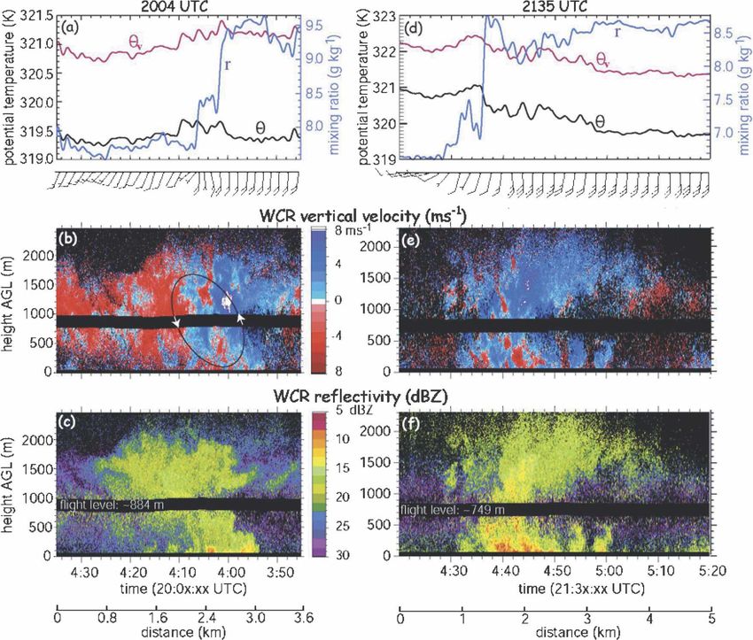
4162 MONTHLY WEATHER REVIEW VOLUME 135
to be answered is whether the density contrast in the ground-based radars were used to place the WCR
CBL is responsible for meso-␥-scale convergence and transects in the context of radar fine lines. Data from
fine-line formation. The null hypothesis is that the pres- both aircraft dropsondes and ground-based balloon
ence and strength of convergence lines is independent sondes, collected in close proximity to the fine lines,
of the density contrast. This question can regard any were used to determine the CBL depth and airmass
radar fine line, but this study focuses on humidity contrast.
boundaries, that is, drylines.
Much attention has been devoted to the finescale b. Density-gradient-driven circulations
horizontal structure of several IHOP fine lines, espe- Radar fine lines are a manifestation of sustained lin-
cially the structure and evolution of misocyclones (Ar- ear convergence within the CBL (Wilson et al. 1994;
nott et al. 2006; Markowski and Hannon 2006; Murphey Geerts and Miao 2005). The central hypothesis of this
et al. 2006; Xue and Martin 2006; Marquis et al. 2007). paper is that this convergence primarily results from a
This along-line variability is not examined here, but we horizontal difference in buoyancy and thus in virtual
are aware that it modulates the flow, convergence, and potential temperature (). The horizontal scale of this
vertical motion along the fine line, and thus may largely convergence and difference (⌬) needs to be deter-
explain the difference between successive cross sections mined. Positive anomalies are buoyant; that is, they
across the line. tend to rise spontaneously, at least if they are rather
The methodology is summarized in section 2. Two small scale (e.g., Houze 1993, p. 225; Doswell and
case studies are presented in section 3. Section 4 syn- Markowski 2004). Buoyant ascent implies a horizontal
thesizes and dynamically interprets findings from these vorticity dipole (viewed in a vertical cross section) and
case studies plus two Verification of the Origin of Ro- roughly circular features (viewed on a map) with a di-
tation in Tornadoes Experiment (VORTEX) cases. ameter of O(1 km), depending on the CBL depth (e.g.,
Stull 1988, p. 461). These features should be present
2. Methodology irrespective of the spatial organization of thermals, that
is, whether or not the thermals are aligned by horizon-
a. Data sources and processing
tal convective rolls (HCRs).
This study primarily uses data collected aboard the A horizontal gradient also drives a convergent so-
University of Wyoming’s King Air (WKA) aircraft. We lenoidal circulation that may lead to a density current,
examine data from 30–40-km-long transects across fine whereby the less dense air is forced over the denser air.
lines at elevations ranging between 150 and 1600 m In this case the buoyancy-induced horizontal vorticity is
above ground level (AGL), in particular the gust-probe a single extreme, although under suitable ambient
winds along the flight track (roughly normal to the fine shear, a vorticity dipole may be present across the
line) as well as water vapor mixing ratio (r) and poten- boundary (e.g., Rotunno et al. 1988). As will be illus-
tial temperature (). Water vapor is measured by a trated below, such a singular extreme or dipole has a
rapid-response Lyman-alpha probe, which was cali- horizontal scale larger than that of thermals. Also, fea-
brated by a slow-response chilled-mirror dewpoint sen- tures tend to be elongated on a map since, to first order,
sor. the secondary circulation is 2D. The circulation pro-
The WKA carried the 95-GHz (W band) Wyoming duces a radar fine line, which separates the air masses
Cloud Radar (WCR). The WCR simultaneously oper- of different density.
ated two fixed antennas, primarily in profiling (up/ The slope of this fine-line echo, and of the associated
down) or vertical-plane dual-Doppler (VPDD) modes updraft in a vertical plane, is evidence of wind shear
(Fig. 2 in Geerts et al. 2006). In the profiling mode, (u/z), which can be large scale or local. If it is large
radar data portray the vertical structure of the CBL scale, all echo/updraft plumes should be tilted. A tilted
over its entire depth except for an ⬃220-m-deep blind echo/updraft plume at the boundary only, surrounded
zone centered at flight level. The VPDD mode allows by upright thermals, is evidence of local baroclinicity at
an estimation of the along-track two-dimensional (2D) that boundary. The Lagrangian change (D/Dt) of hori-
air circulation below the aircraft at a resolution of ⬃30 zontal vorticity () due to baroclinicity can be esti-
m. The extraction of the echo motion from the Doppler mated as
velocity measured from a moving platform, and the
D g ⭸
dual-Doppler synthesis, are discussed in Damiani and ⫽ , 共1兲
Haimov (2006). Dt ⭸x
Several other IHOP data sources were used. Low- where x is the boundary-normal direction [in the cases
elevation-angle reflectivity from various scanning examined here, pointing (south)east], ⫽ (u/z) ⫺ (w/x),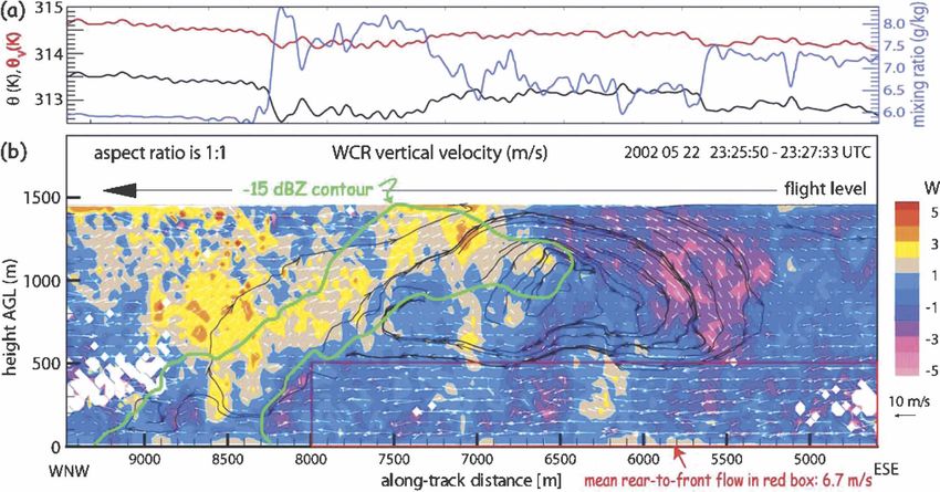
DECEMBER 2007 MIAO AND GEERTS 4163
FIG. 1. Differences in along-track (approximately cross dryline) wind (gray symbols) and
(black symbols) across two drylines documented during VORTEX, and best linear fit
(dashed lines): (a) 6 May 1995 (Atkins et al. 1998; Ziegler and Rasmussen 1998); (b) 7 Jun
1994 (Ziegler and Rasmussen 1998). The differences are defined as moist (x ⬎ 0) minus dry
(x ⬍ 0), and are computed from 10-km averages on either side of the dryline, for flight legs
at various levels. The data were collected at 1-Hz frequency aboard the NOAA P-3
aircraft. The CBL depths listed are derived from Fig. 17 of Atkins et al. (1998) for (a) and
Fig. 9 of Ziegler and Rasmussen (1998) for (b).
w is vertical velocity, and g is gravitational acceleration. perimentation has yielded the following objective cri-
In the cases examined below, the length scale is greater teria for sounding data: h is at the base of the layer
than the height scale (the depth of the CBL h) by a where (d/dz) ⬎ [0.5 K (200 m)⫺1] and (d/dz) ⬎ [1.0 K
factor of 2 or more; thus, wind shear dominates . In (1000 m)⫺1], and nowhere within the 1000-m layer does
what follows we assume along-boundary uniformity decrease by over 0.2 K. The CBL depth on the denser
(/y ⫽ 0). To start, we treat (1) as an initial value side of the dryline (hde) often is considerably less than
problem and examine the development of shear (uh ⫺ the depth on the lighter side (hli) (e.g., Fig. 17 in Atkins
u0)/h within an initially motionless CBL as a result of a et al. 1998). In the two dryline cases shown in Fig. 1, hli
steady gradient ⌬ /⌬x, during a period ⌬t. Initially, (on the dry side) was 2–3 times larger than hde. Flight
advection by the baroclinically generated flow can be levels higher than that shown in Fig. 1 were not flown,
ignored. Thus (1) can be integrated vertically and in but linear extrapolation of ⌬ data shown in Fig. 1
time to obtain suggests that ⌬ nearly vanishes at hde. The ratio of ⌬
at hde to ⌬,0 is defined as R, that is,
冕
h
u h ⫺ u0 ≅
g⌬t
0
⌬
⌬x
dz, 冋
⌬ ≅ ⌬,0 1 ⫺ 共1 ⫺ R兲
z
hde册. 共2兲
For the cases shown in Fig. 1 and in section 3a, R
where is the average over 0 ⬍ z ⬍ h. The ⌬ averages 0.37, ranging between 0.20 and 0.51. The
driving this circulation is largest near the ground above integral can be solved over 0 ⬍ z ⬍ hde using (2),
(where it is referred to as ⌬,0) and decreases with and the shear can then be estimated as
height, as illustrated in Fig. 1 for two dryline cases de-
uhde ⫺ u0 共1 ⫹ R兲g⌬t ⌬,0
scribed in the literature, and as confirmed in section 3a ≅ . 共3兲
below. hde 2 ⌬x
The CBL depth h is defined as the level where po- This approximation is useful only in the initial stages
tential temperature starts to increase with height. Ex- (⌬t small), before frictional dissipation and advection4164 MONTHLY WEATHER REVIEW VOLUME 135
冕
become important. Later, an equilibrium develops, in hde
which the steady-state secondary circulation (a form of 2⌬xg ⭸
⫺⌬u20共1 ⫺ Ru 兲 ≅ dz
kinetic energy) tries to destroy the horizontal ⌬ (a ⭸x
0
form of potential energy) that is maintained by advec-
tion and/or surface heat fluxes. The convergence asso- or
ciated with this circulation can be estimated as follows,
冕
starting with (1): hde
1 ⌬xg ⭸
g ⭸ D ⭸ 2u ⭸ 2u ⫺⌬u0 ≅ dz. 共5兲
1 ⫺ Ru u0 ⭸x
⫽ ⫽u ⫹w 2. 0
⭸x Dt ⭸x⭸z ⭸z
That is, the tendency term is ignored in the total de- In the absence of “ambient” flow, u0 merely is the hori-
rivative. The above relationship can be integrated over zontal component of the solenoidal circulation. Using
hde: (2), (5) can be approximated as follows:
共1 ⫹ R兲ghde⌬,0
冕 冕 冕
hde hde hde
g ⭸ ⭸ 2u ⭸2u ⫺⌬u0 ≅ , 共6兲
dz ⫽ u dz ⫹ w dz. 2共1 ⫺ Ru兲u0
⭸x ⭸z⭸x ⭸z 2
0 0 0
where the subscript “0” refers to measurements near
We now apply the chain rule twice, and assume 2D the surface, in practice below 0.5hde. The magnitude of
incompressible continuity [(u/x) ⫹ (w/z) ⫽ 0] and the confluence ⌬u0 in (6) is affected by the rates of
w ⫽ 0 at z ⫽ 0 and z⫽ hde, to modify the right-hand side decline of ⌬ and ⌬u with height in the CBL affect, and
of the above equation as follows: by u0. In general, Ru should be close to zero, since
diffluent return flow should occur in the upper CBL;
冕 冕
hde hde
⭸2 u ⭸2u however, the density contrast can be found over a
u dz ⫹ w dz greater depth. In practice, u0 is calculated as the aver-
⭸z⭸x ⭸z2
0 0 age low-level flow on the “dense” side of the boundary,
minus the “ambient” flow (defined as the average low-
冕 冏 冕
hde hde
⭸ 2u ⭸u hde ⭸w ⭸u level boundary-normal flow in nearby soundings on op-
⫽ u dz ⫹ w ⫺ dz posite sides of the boundary), and is positive toward the
⭸z⭸x ⭸z 0 ⭸z ⭸z
0 0 boundary. Note that u0 is in the denominator of (6);
when u0 is small, as with some weak boundaries, its
冕 冕
hde hde
⭸ 2u ⭸u ⭸u uncertainty can make confluence estimates based on
⫽ u dz ⫹ dz (6) unreliable.
⭸z⭸x ⭸x ⭸z
0 0 Expression (6) fundamentally is an application of the
Bjerknes circulation theorem (Bjerknes 1898) and re-
冕 冏 冕
hde hde
⭸ 2u ⭸u hde ⭸ 2u lates the steady-state low-level cross-boundary conflu-
⫽ u dz ⫹ u ⫺ u dz. ence (⫺⌬u0) to ⌬,0 at corresponding horizontal scale.
⭸z⭸x ⭸x 0 ⭸z⭸x
0 0 The term ⫺⌬u0 is similar to convergence, but it does
not imply a scale (⌬u0 is not divided by ⌬x), and the
The first and third terms cancel. Thus,
along-boundary component ( /y) is ignored. A simi-
冉 冊 冉 冊 冕
hde lar expression has been obtained by Grossman et al.
⭸u2 ⭸u2 g ⭸ (2005), but they start from a circulation integral, and
⫺ ⫽ dz. 共4兲
2⭸x hde 2⭸x 0 ⭸x ignore the variation of ⌬ with height.
0
Another relationship between confluence and den-
Observations indicate that the boundary-normal con- sity contrast can be obtained from density current
fluence is strongest near the surface and, by extrapola- theory. The boundaries examined herein may not have
tion, vanishes near hde. The average ratio of ⌬u at hde to a sufficient ⌬ to drive a classic atmospheric density
⌬u0, defined as Ru, is only 0.17 for the cases illustrated current, as documented for instance for thunderstorm-
in Fig. 1 and section 3a. Thus, ⌬u vanishes at a slightly generated gust fronts (e.g., Mueller and Carbone 1987)
lower level than ⌬. For simplicity we use the same or cold fronts (e.g., Wakimoto and Bosart 2000); nev-
linear expression (2) for the profiles of ⌬u and ⌬u2, but ertheless, the theory may apply. Laboratory experi-
with a slope Ru. Then a finite-difference expression of ments suggest that the speed of a density current (Udc)
(4) becomes can be estimated as follows (Simpson and Britter 1980):DECEMBER 2007 MIAO AND GEERTS 4165
Udc ⫽ K 冑 gDdc⌬
⫹ bUenv. 共7兲
the same horizontal scale. The main difference is that in
the case of a solenoidal vortex (6), | ⌬u | ⬀ hde⌬,0,
while in the case of a density current (9), | ⌬u | ⬀ 公hd-
This equation is based on the horizontal momentum e⌬,0.
conservation equation (e.g., Houze 1993); Udc bears Even though the term ⌬x does not appear in either
similarity to the shallow water wave speed. Some form (6) or (9), the horizontal scale over which these differ-
of (7) is commonly encountered in the literature, in- ences are computed clearly matters. The question of
cluding in atmospheric applications. In (7) K corre- scale was raised by Atkins et al. (1998) and is further
sponds with the Froude number; experimental values explored here. WKA wind and thermodynamic data
for K range from 0.7 to 1.0 or higher for atmospheric are averaged over either ⌬x ⫽ 3 km or ⌬x ⫽ 10 km on
density currents (e.g., Wakimoto 1982; Mueller and either side of the leading edge of the boundary along all
Carbone 1987; Kingsmill and Crook 2003); Uenv is the available low-level flight legs (below 0.5hde). The aver-
ambient low-level flow normal to and ahead of the den- aging is necessary in order to reveal small differences
sity current. Laboratory work by Simpson and Britter (the signal) embedded in much larger perturbations of
(1980) indicates that b ⫽ 0.70. Numerical work by Liu convective origin (the noise). The choice of these scales
and Moncrieff (1996) suggests that b ⫽ 0.74, ranging is based on the following. A distance of 3 km should
between 0.71 and 0.78. The density current depth (Ddc) exceed the diameter of most coherent eddies (thermals)
is assumed to be equal to hde, although this is uncertain in the fair-weather CBL: aircraft data (e.g., Kaimal et
(see section 4d below). The difference normally is al. 1976) and WCR vertical profile data (Miao et al.
measured on the ground; therefore ⌬,0 is used in (7). 2006) indicate that in the mid-CBL the diameter of
The movement of a boundary provides poor evi- most eddies is 1.5h or less. However HCRs generally
dence for the density-current nature of the boundary have wavelengths longer than 3 km, and 10 km is about
(e.g., Smith and Reeder 1988). First, the estimation of the maximum flight track distance generally (but not
the observed motion of the boundary is complicated by always) available on either side of the boundary in
along-line variability. Second, the estimation of the IHOP. The distance between the centers of the aver-
theoretical boundary motion using (7) has several un- aging domains on either side of the dryline equals the
certainties, including the determination of the “ambi- averaging distance ⌬x, because we do not assume a
ent” low-level flow Uenv. This determination is compli- buffer zone around the boundary. The third and largest
cated by the ambient wind shear and variable CBL scale is the boundary-normal distance between sound-
depth. ings. In the cases examined here, this distance (⌬x)
We can however measure the flow confluence (⫺⌬u) ranges from 15 to 62 km. Sounding data differences are
with some accuracy, and it can be compared with the computed based on averages between the ground and
following estimate from density current theory. First, 0.5hde.
observations have shown that the feeder flow (Umax) The theory is tested first for a vigorous but shallow
exceeds the density current speed by about 40% cold front observed on 24 May 2002 in west Texas (Xue
(Simpson et al. 1977), and Martin 2006; Karan and Knupp 2006). This cold
front had all the characteristics of a density current
Umax ≅ 1.40Udc. 共8兲
(Geerts et al. 2006): large ⌬,0 values (3–6 K over
Thus the confluence normal to a density current, scales of 3–19 km) and strong convergence (⫺⌬u) at the
⫺⌬Udc, can be inferred from (7) and (8), assuming K ⫽ head (8–11 m s⫺1 over the same scales) (Table 1). Both
0.85 and b ⫽ 0.74: the solenoidal vortex Eq. (6) and the experimental den-
sity current Eq. (9) overestimate the low-level conflu-
⫺⌬Udc ⫽ Umax ⫺ Uenv
ence at all scales, compared to observed values (Table
≅ 1.19 冑 gDdc⌬,0
⫹ 0.04Uenv
1).
3. Fine-line observations
≅ 1.19 冑 ghde⌬,0
. 共9兲
Two case studies are presented below. Case studies
of two other drylines in IHOP, on 24 May and 18 June
2002, can be found in Miao (2006).
The neglect of the term 0.04Uenv implies an uncertainty
⬍1 m s⫺1, which is less than other sources of error in
a. 22 May dryline
this estimation. Both (6) and (9) relate the steady-state On 22 May 2002 the IHOP armada studied a dryline
near-surface cross-boundary confluence to ⌬,0 over fine line near the S-band dual-polarization Doppler ra-4166
TABLE 1. Analysis of the horizontal difference (⌬) and confluence (⫺⌬u) for several fine-line boundaries, all with a humidity gradient, and comparison with theoretically
estimated confluence values. The latter either assumes a steady solenoidal circulation [⫺⌬u0, see Eq. (6) in section 2b] or a density current [⫺⌬Udc, see Eq. (9)]. The factor R and
Ru in (6) are set at 0.37 and 0.17, respectively; these are averages for the profiles of ⌬ and ⌬u on 22 May 2002, 6 May 1995, and 7 Jun 1994. The differences are scale dependent,
and three different scales are assumed: flight-level WKA data are averaged over either 3 or 10 km on either side of the boundary (defined as the location of strongest humidity
gradient), or the distance between two soundings on opposite sides of the boundary is used, if available. Only flight legs below 0.5hde are used. Sounding data (“sonde”) are averaged
between the surface and 0.5hde. The distance between soundings is calculated normal to the boundary. Here u0 is the mean boundary-normal flow on the dense side, minus the
“ambient” low-level flow (positive toward the boundary).
Predicted Predicted Observed
Boundary Scale ⌬r ⌬ hde u0 ⫺⌬u0 ⫺⌬Udc ⫺⌬u
Date [dryline (DL)] Source (km) (g kg⫺1) (K) (m) (m s⫺1) (m s⫺1) (m s⫺1) (m s⫺1) Comments
22 May Primary DL WKA 3 2.7 ⫺1.03 1600 5.8 7.3 8.4 4.0 Average of five flight legs between 2222 and 0009 UTC;
see Fig. 6
WKA 10 3.0 ⫺1.33 6.0 9.1 9.6 4.7 Average of three flight legs between 2222 and 0009 UTC
Secondary DL WKA 3 1.4 ⫺0.02 2.7 0.3 1.2 1.4 Average of the 2223 and 2355 UTC DL crossings; see
Fig. 4
Both DLs Sonde 62 5.2 ⫺4.46 7.7 23.8 17.5 8.9 See Fig. 1
24 May Western DL WKA 3 1.7 ⫺0.29 1320 2.7 3.7 4.1 3.9 Average of two flight legs: one at 170 m AGL at 1948
UTC (see Fig. 9 of Weckwerth et al. 2004) and one at
400 m AGL at 1937 UTC (see Fig. 8 of Geerts et al.
2006)
WKA 10 1.3 ⫺0.24 4.5 1.8 3.7 3.3 Same as above, but second leg extends only 6 km into
dry air
Eastern DL WKA 3 1.9 ⫺0.46 1200 2.7 5.2 4.9 4.3 One flight leg at 200 m AGL at 2047 UTC
MONTHLY WEATHER REVIEW
WKA 10 2.2 ⫺0.54 2.8 5.9 5.3 4.8 Same as above, but extending only 8 km into dry air
Sonde 27 3.3 ⫺0.72 4.2 5.3 6.4 4.9 Dry side: 2032 UTC Learjet dropsonde, 9 km west of the
DL; moist side: 2035 UTC Learjet dropsonde, 18 km
east of the DL
Cold front WKA 3 — 2.90 800 5.4 11.3 10.0 7.8 Same flight legs as for primary dryline; cold front moves
at ⬃7 m s⫺1 to the southeast (Geerts et al. 2006)
WKA 10 — 4.11 6.4 13.4 11.9 9.1 Same as above, but first leg only has 5 km in the cold air,
and second leg only 6 km into the warm air
Sonde 19 — 6.14 7.7 16.6 14.5 10.6 See Fig. 6 of Geerts et al. (2006)
VOLUME 135DECEMBER 2007
TABLE 1. 具Continued)
Predicted Predicted Observed
Boundary Scale ⌬r ⌬ hde u0 ⫺⌬u0 ⫺⌬Udc ⫺⌬u
Date [dryline (DL)] Source (km) (g kg⫺1) (K) (m) (m s⫺1) (m s⫺1) (m s⫺1) (m s⫺1) Comments
18 Jun Early phase WKA 3 2.1 ⫺0.35 1020 3.2 2.8 3.9 2.5 Average of seven flight legs below 0.5zi, between 1837
and 2138 UTC
WKA 10 2.8 ⫺0.84 3.7 5.9 6.1 3.0 Average of six flight legs below 0.5zi, between 1836 and
2115 UTC
Sonde 32 3.1 ⫺1.94 5.8 8.6 9.2 3.9 Dry side: 2022 UTC Mobile GPS/Loran Atmospheric
Sounding System (M-GLASS) sounding, 11 km west
of the DL; moist side: 2042 UTC M-GLASS sounding,
23 km east of the DL
Late phase WKA 3 2.4 ⫺0.41 1500 6.4 2.4 5.1 1.7 Average of two flight legs below 0.5zi, between 2326 and
primary DL 2341 UTC
WKA 10 3.1 ⫺0.87 7.6 4.3 7.5 2.2 Same as above
Sonde 15 2.3 ⫺1.05 7.1 5.6 8.2 3.0 Based on 2127 UTC (dry) and 2144 UTC (moist)
M-GLASS soundings
Late phase WKA 3 2.2 ⫺0.19 4.0 1.8 3.5 5.5 Average of two flight legs below 0.5zi, between 2330 and
secondary DL 2337 UTC
WKA 10 2.6 ⫺0.46 4.7 3.7 5.4 5.7 Same as above
19 Jun Early phase WKA 3 1.2 0.32 1610 2.7 4.7 4.7 6.1 Based on two flight legs below 500 m AGL, both before
MIAO AND GEERTS
DL (dry side 2000 UTC; see Fig. 12
cooler) WKA 10 1.4 0.75 3.2 9.4 7.2 7.2 Same as above, but some leg length limits; see also
Table 2 in SG07
Sonde 18 2.0 0.59 3.6 6.6 6.4 7.7 See Fig. 7a
Late phase DL WKA 3 1.5 ⫺0.49 1380 4.1 4.1 5.4 7.1 Based on two flight legs below 500 m AGL, after
(moist side 2100 UTC
cooler) WKA 10 2.9 ⫺0.66 3.2 7.2 6.3 8.3 Same as above, but some leg length limits; see also
Table 2 in SG07
Sonde 38 3.8 ⫺0.89 6.7 4.6 7.3 9.1 See Fig. 7b
7 Jun 1994 VORTEX DL NOAA 10 4.7 ⫺1.9 1500 6.1 11.8 11.1 9.4 Six flight legs below 600 m AGL, between 2220 and
P-3 2348 UTC
6 May 1995 VORTEX DL NOAA 10 5.7 ⫺1.8 1300 7.0 8.8 8.2 7.0 Five flight legs at ⬃180 m AGL, between 2146 and
P-3 2358 UTC
41674168 MONTHLY WEATHER REVIEW VOLUME 135
considerable (Fig. 3; as well as Fig. 4 in Demoz et al.
2006); the air mass between the two drylines had inter-
mediate properties. The soundings shown in Fig. 3 in-
dicate that the moist-air was 4.5 K lower than that on
the dry side (Table 1). Even larger differences across
the dryline complex existed at the surface (Fig. 2). The
dry-side CBL was remarkably deep, and about twice as
deep as the moist-side CBL depth (hde), which is too
deep for the CBL depth to be inferable from WCR
profiles (Miao et al. 2006); the temperature of the up-
per ⬃1 km of this CBL was below the threshold of most
insects. But east of the eastern dryline, WCR-inferred
CBL heights corresponded well with the thermody-
namic CBL height (Fig. 4).
Clear-air reflectivity imagery, for instance from S-
FIG. 2. Radar reflectivity and surface station observations near Pol, indicates that the convergence zone of the primary
the dryline (DL) on 22 May 2002. The reflectivity field, ranging dryline had a sharply defined western edge and a more
from ⫺5 (black) to ⫹30 dBZ (white), is from the 0.5° scans of the
fuzzy eastern edge (Fig. 2; top panels of Fig. 2 in Demoz
Amarillo, TX (AMA), WSR-88D and S-Pol radars. Here (K)
and r (g kg⫺1) are plotted instead of the conventional temperature et al. 2006; Fig. 4a in Weiss et al. 2006). This contrast is
and dewpoint. A full barb is 5 m s⫺1. The time shown in the upper most apparent at greater radar range, where S-Pol
left applies to the station data. Radar data were collected within sampled the upper CBL. That suggests that lofted in-
a few minutes of this time. sects were carried eastward over moist-air wedge. In
other words, westerly shear across the dryline (Fig. 3)
dar (S-Pol) in the Oklahoma Panhandle. Two fine lines tilted the dryline updraft eastward and caused an east-
developed: a more defined one to the east (the “pri- ward trailing echo anvil.
mary dryline”) and a less apparent line to the west (Fig. This eastward tilt of both fine lines is apparent in
2; Fig. 3 in Weiss et al. 2006). These lines merged north transects of WCR reflectivity, for instance at 2220 and
of the IHOP operations. The humidity and temperature 2243 UTC (Fig. 4). The echo anvil is most obvious east
contrasts between the moist and dry air masses were of the eastern dryline at 2243 UTC (Fig. 4h). The air
FIG. 3. Profiles of r and derived from two near-simultaneous soundings released on opposite sides
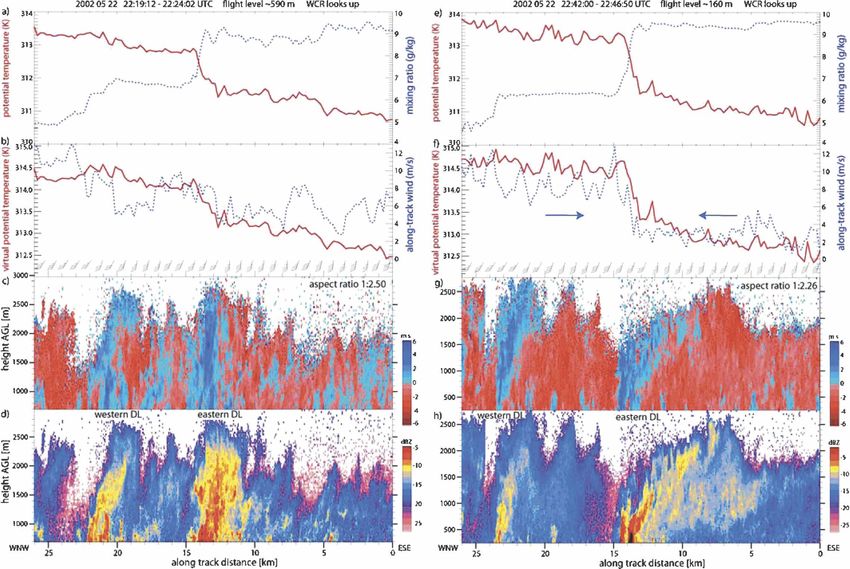
of the 22 May 2002 split dryline. Gray (black) lines and symbols refer to the moist (dry) side.DECEMBER 2007 MIAO AND GEERTS 4169 FIG. 4. WKA observations of the 22 May dryline (DL) system, along two transects, on the left around 2220 UTC (flight level ⬃590 m AGL), and on the right around 2243 UTC (flight level ⬃160 m AGL). The horizontal axis is distance along the flight track; the reference point (x ⫽ 0) is arbitrary but is the same in both transects. In this and other transects, the moist side is on the right. (a), (b), (e), (f) Flight-level data are shown on top. This includes the along-track (dryline normal) wind and the horizontal wind barbs (full barb ⫽ 5 m s⫺1). Along-track flow convergence occurs when the blue trace descends from left to right in (b) and (f), and the main convergence belt is highlighted by the opposing blue arrows. (c), (g) WCR vertical velocity (positive values indicate ascent), and (d) and (h) corresponding WCR reflectivity in the vertical plane above the aircraft. In the WCR plots the vertical axis (height) is exaggerated somewhat (see “aspect ratio”); this makes the tilt of plumes less apparent. was moister and cooler on the east side of both lines, 1.0 K over 3 km, and 1.3 K over 10 km (Table 1). No but the eastern line, with higher reflectivity values, had measurable local gradient exists across the secondary a larger temperature and humidity contrast, as well as western dryline. (Only 3-km averages are available for more convergent flow. The latter is evident from the this boundary.) The 10-km ⌬ across the primary gust probe wind normal to the dryline (Figs. 4b,f), and dryline is only 30% of the ⌬ across 62 km (Table 1), from the WCR vertical velocity field (Figs. 4c,g). The implying a broader (meso-) gradient. flight-level along-track confluence resulted from slight The updraft tilt is consistent with the gradient changes in the direction of a strong wind, mainly across across the primary dryline; that is, it appears to be due the eastern dryline (see wind barbs in Figs. 4b,f): the to baroclinically generated horizontal vorticity. The wind in the CBL generally blew at ⬃20 m s⫺1 from the weak gradient across the western dryline may explain south-southwest, along the dryline, but east of the why this line gradually disappeared, mostly between dryline it was more southerly and stronger. The eastern 2220 and 2320 UTC (e.g., Fig. 2 in Demoz et al. 2006). line was especially marked by strong updrafts, up to ⬃5 A cross-dryline circulation was well established at m s⫺1. The dryline echoes penetrated well above hde 2326 UTC (Fig. 5). A 6.7 m s⫺1 strong rear-to-front (Figs. 4d,h; Fig. 9 in Weiss et al. 2008), notwithstanding current (highlighted in the red box in Fig. 5b) advected the low temperature near the echo tops (12°C at 2700 m low- air toward the leading edge, which was tilted AGL). about 45° from vertical. Because the primary dryline The gradient across the primary dryline is about was quasi stationary at this time, the flow shown in Fig.
4170 MONTHLY WEATHER REVIEW VOLUME 135 FIG. 5. (a) WKA flight-level data and (b) WCR vertical-plane dual-Doppler wind field across the 22 May primary dryline around 2326 UTC. The vector field is visually enhanced by objectively drawn streamlines (black lines with arrows). The vertical velocity field is shown in color. The nadir antenna ⫺15-dBZ contour, enclosing the strongest echoes, is shown in green. 5b can be thought of as relative to the boundary, which moist-side temperature and wind profiles on 22 May resembled a density current head. At flight level (from the sounding shown in Fig. 1), filtered to a ver- (⬃1540 m AGL) this head was intercepted between tical resolution of 100 m (as done in Geerts et al. 2006), 7300 ⬍ x ⬍ 8200 m (Fig. 5b); air in this region had r and yield a minimum Ri of 0.4 just above hde. KH instability values between those characterizing the dry and the occurs when Ri ⬍ 0.25 (e.g., Miles and Howard 1964; moist air masses at lower levels (Fig. 4e). This confirms Mueller and Carbone 1987). Thus the deficit of the observations by Ziegler and Hane (1993) that the head 22 May dryline density current appears insufficient, or is a mixing zone. One mixing mechanism must be the rather the resulting shear at the interface is too weak, to recirculation of flow into the head: to the rear of the generate breaking KH waves. head, a strong downdraft mixes air into the rear-to- The horizontal vorticity within the ⬃1-km-diameter front current (Fig. 5b). At the time of the WKA cross- solenoid highlighted by black streamlines in Fig. 5b is ing, the air in the head was generally rising but nega- about 2 ⫻ 10⫺2 s⫺1. An earlier VPDD transect, at 2201 tively buoyant (Fig. 5a). This negative buoyancy and UTC (1.4 h earlier), showed no coherent circulation the strong downdraft behind the head are additional across the dryline; at that time the dryline plume was indications of density current dynamics. essentially upright. Flight-level data from the primary- Farther east of the primary dryline the moist air was dryline crossings below 0.5hde show a steady increase of sampled intermittently at flight level (not shown), ⌬ over 3 km from 0.69 to 1.31 K between 2222 and which roughly corresponds with hde (Figs. 4d,h; Fig. 1). 2356 UTC. The mean gradient [1.03 K (3 km)⫺1; Thus the CBL top had undulations, possible trapped Table 1] can produce the observed horizontal vorticity lee waves behind the density current head (e.g., Weck- in 0.75 h, according to (3). Thus the circulation at 2326 werth and Wakimoto 1992; Jin et al. 1996). The WCR UTC (Fig. 5b) could have been generated in the time reflectivity profiles reveal no evidence of breaking available and may have become rather steady. Even Kelvin–Helmholtz (KH) waves. Such waves were ob- during the short time period between 2220 and 2243 served in the case of the 24 May cold-frontal density UTC an increase in echo tilt of the primary dryline is current, marked by a thrice-stronger gradient over 10 apparent (Figs. 4d,h) and, correspondingly, an increase km (Table 1). In that case the minimum value of the in gradient and in confluence. (It is possible that this Richardson number (Ri) at the interface between difference between the two transects in Fig. 4 is not a denser and lighter air was ⬃0.1 (Geerts et al. 2006). The uniform temporal change but is rather due to along-line
DECEMBER 2007 MIAO AND GEERTS 4171
variability advecting into the geographically fixed track WCR transects and flight-level data support the notion
from the south.) Between 2300 and 0000 UTC, the pri- of a density current, with a well-defined leading head
mary dryline began to retrograde (move westward), at and low-level rear-to-front flow. Density current char-
a speed of 2–3 m s⫺1 by 0000 UTC. acteristics are evident in all WKA/WCR transects ex-
Vertical variations of the airmass difference across cept the earliest one, notwithstanding significant along-
the 22 May primary dryline are shown in Fig. 6. In all line variability and an along-line flow far stronger than
transects the moist air mass is sufficiently cooler, such the solenoidal circulation.
that it is also denser. Both ⌬r and ⌬ decrease with
b. 19 June dryline
height, as do the VORTEX drylines (Fig. 1), but the
level where the extrapolated ⌬r and ⌬ values reach On 19 June 2002 the IHOP armada examined a syn-
zero is lower, only slightly above hde. The flow is con- optic-scale frontal shear zone in northwest Kansas
vergent in all transects except one1 (Fig. 6c), and ⌬u (Murphey et al. 2006; SG07). Weak southwesterly flow
also tends to be strongest at low levels. The dry air rises converged at a prefrontal dryline with a southerly low-
relative to the moist air in most transects, especially at level jet confined in the moist air mass (Fig. 7). Deep
low and middle levels (Fig. 6c). The slopes of ⌬ and convection erupted along the dryline near 2130 UTC, in
⌬u are used in the estimation of R and Ru [Eq. (6); particular in the vicinity of misocyclones that modu-
Table 1]. lated the moisture and vertical velocity field (Murphey
The dryline convergence zone (DCZ) can be several et al. 2006; Marquis et al. 2007). These misocyclones
kilometers wide yet the term humidity “discontinuity” resulted from strong horizontal wind shear across the
is appropriate at the scale of the coherent eddies cap- dryline, far stronger than on 22 May. This is evident by
tured by the WCR. The rapid change in r is evident in comparing the flight-level wind barbs in Fig. 4 to those
Figs. 4a,e, and the horizontal gradient ⌬r/⌬x averaged in Fig. 8. SG07 have shown that the dryline updraft and
over 300 m (Fig. 6d) across the dryline is almost 10 echo plume tilted toward the west in an early phase,
times as large as that averaged over 3 km (Fig. 6a), and when the dryline progressed eastward, and later their
nearly the entire humidity change is concentrated in slope reversed, toward the moist side, while the dryline
300 m. Yet the change is less discontinuous: ⌬ /⌬x became quasi stationary. The change in slope of the
over 300 m (Fig. 6d) is only 3 times larger than that over updraft was accompanied by a circulation reversal.
3 km (Fig. 6b). The presence of a humidity jump Soundings were collected on both sides of the dryline,
sharper than the change generally applies to the in relative proximity to the dryline, both in the early
other IHOP cases studied here; data for the two and later phases (Fig. 7). Initially was slightly lower
VORTEX cases shown in Fig. 1 do not allow this fines- on the dry side, which is unlike any dryline reported on
cale comparison. in this study, but has been recorded before (Fig. 4 in
The observed cross-dryline confluence (⫺⌬u0) is Crawford and Bluestein 1997). In the course of ⬃1.5 h,
compared to the one expected assuming a steady-state between 1330 and 1500 local solar time, the CBL
solenoidal circulation (6) and a density current (9) (sec- warmed and deepened on the dry side, resulting in a
tion 2b) in Table 1. Both theoretical estimates are high lower mixing ratio, due to the entrainment of dry free-
(as for the 24 May cold front), and far higher than tropospheric air into the deeper CBL. Yet on the moist
observed at a length scale of 62 km, indicating that (6) side the stable layer above the CBL subsided, and the
and (9) do not apply at a larger scale in the presence of CBL temperature and humidity changed little. As a
a large-scale gradient. This agrees with the dryline result, the humidity and mainly temperature contrasts
study of Atkins et al. (1998): they find that density cur- across the dryline increased, and the net effect was that
rent theory can be applied at 5 km, but not at 50 km. air on the moist side became denser.
In summary, the moist air mass just east of the 22 In both phases the updraft and echo slopes are dy-
May primary dryline developed a deficit of sufficient namically consistent with the observed buoyancy gra-
magnitude to drive solenoidal circulation with sloping dient across the dryline: in the early phase air on the dry
updraft and an echo plume trailing toward the moist air. side is denser (Fig. 8a), but as the dry side warms faster
than the moist side, the gradient has a reversed sign
in the late phase (Fig. 8d). The transition from a west-
1
The one exception (at 2201 UTC, at a flight level of 1470 m) ward-tilted boundary, with denser air on the dry side, to
could be discounted because, even though there is a small humid-
an eastward-tilted dryline with denser air on the moist
ity difference (0.6 g kg⫺1), the CBL is shallower at this time, the
⌬ values are insignificant, both at flight level (0.23 K) and on the side is examined further in Fig. 9, using WKA data
ground (⬍0.5 K), and the density current circulation is not yet within the CBL. Some drying occurs during the early
present, as mentioned above. afternoon, but the humidity difference persists. Thus4172 MONTHLY WEATHER REVIEW VOLUME 135
FIG. 6. Profiles of the difference between moist and dry air on 22 May, based on in situ
WKA data at various flight levels between 2207 and 2350 UTC. The difference (moist ⫺
dry) is based on 3-km averages, on opposite sides of the primary dryline, which was marked
by a clear humidity gradient. The top of the vertical axis is hde ≅ 1.6 km (Fig. 3). Black plus
symbols refer to the lower axis and gray stars to the upper axis. The dryline-normal wind
(u) and vertical air motion (w), shown in (c), are obtained from the gust probe. In (d) the
maximum gradient at the dryline is shown, over ␦x ⫽ 300 m, for 100-m filtered values.
Dashed lines indicate linear best fits.DECEMBER 2007 MIAO AND GEERTS 4173
FIG. 7. As in Fig. 3, but for the 19 Jun 2002 dryline: (a) early phase ( higher on the
moist side); (b) late phase, nearly 1.5 h later ( higher on the dry side). Note the corre-
spondence of the x axes in (a) and (b).
the reversal of the gradient is entirely due to differ- was interpreted as the result of a solenoidal circulation.
ential warming: the dry-side CBL warms more than the In the early traverses the WCR reflectivity peaks near
moist-side CBL, due to advection and/or surface sen- the humidity jump that marks the dryline and continues
sible heat flux. The ⌬ is small both in the early and the to be high to the west (Fig. 9d), suggesting a solenoidal
late phases, less than 0.5 K at the 3-km scale (Table 1), circulation with upper-CBL transport to the west; dur-
and less than 1.0 K at the 10-km scale and according to ing the last two traverses the lowest reflectivity values
the sounding pairs. So the resulting solenoidal circula- are found to the west, and higher values are found near
tion should be weak. and to the east of the dryline. The WCR vertical veloc-
Indeed, weak solenoidal circulations, weaker than ity pattern is consistent with this (Fig. 9e): in the early
the one observed on 22 May (Fig. 5b) have been docu- (late) phase rising motion tends to occur just east (west)
mented in both phases (SG07), although an updraft/ of the dryline; however, this signal difficult to discern in
downdraft dipole is not always apparent (e.g., Fig. 8e). a vigorously convective BL.
Indirect evidence for the secondary circulation and its Low-level WKA dryline traverses indicate that the
reversal arises from the WCR reflectivity profile across confluence is 6–7 m s⫺1 over 3 km for both phases
the dryline. The higher reflectivity on the moist (Table 1). This is stronger than what can be expected
(denser) side of the 22 May primary dryline (Figs. 2, 4h) from baroclinicity at this scale (6–7 m s⫺1). This applies4174 MONTHLY WEATHER REVIEW VOLUME 135
FIG. 8. Flight-level data and WCR vertical transects above and below flight level for the 19 Jun 2002
dryline, during the (a)–(c) early phase (2004 UTC) and (d)–(f) late phase, 1.5 h later. The flight-level gust
probe wind is shown as barbs above the WCR vertical velocity panel. The direction of the solenoidal
circulation is shown in (b).
at other scales as well (except for the 10-km scale in the strong finescale convergence during all phases of the 19
early phase; Table 1). It is remarkable that it applies June dryline. One possibility is that it was driven by
even to the largest scale: the ⌬u between the two late- buoyancy relative to both adjacent air masses. Such
phase soundings, 38 km apart, is above the two theo- buoyancy, with a ⬘ magnitude of ⬃1 K, was evident
retical ⌬u estimates. As mentioned before (section 3a), from a dropsonde transect (Fig. 13b in SG07) and, on a
the density current confluence at such scale tends to be smaller scale, from a stepped WKA traverse (Fig. 12a in
an overestimate in the presence of a background SG07), both just prior to CI. It is evident also on a scale
gradient. of a few kilometers, although the magnitude is only
Thus some other mechanism may have contributed ⬃0.5 K at 2135 UTC (Fig. 8d). This buoyancy may
to finescale convergence leading to the 19 June dryline explain why mainly ascending motion occurs at this
fine line. Additional evidence for this arises from the time, rather than a solenoidal circulation (Fig. 8e). The
fact that at some time between the two phases illus- flight-level wind field (shown below Fig. 8d) suggests
trated in Fig. 8, ⌬ must have been zero for the rever- strong vertical vorticity near the dryline between 1.2 ⬍
sal to occur. Yet throughout the period, Doppler-on- x ⬍ 2.0 km, roughly collocated with the main updraft in
Wheels (DOW)-3 reflectivity and velocity data indicate the WCR transect. At this time the WKA intersected
that the dryline remained well defined and that the an intensifying misocyclone, labeled “J” in Fig. 6 of
cross-dryline flow was convergent. Horizontal-plane Marquis et al. (2007).
WCR velocity data for an along-dryline flight leg at A second possibility is downward transfer of momen-
2040–2047 UTC indicate strong convergence at ⬍1-km tum toward the dryline, on either side of the dryline,
scale (Fig. 11 in SG07). although evidence presented in section 4b argues
It is not clear what mechanism explains the rather against that process. Third, larger-scale dynamics con-DECEMBER 2007 MIAO AND GEERTS 4175
FIG. 9. Composite of WKA measurements across the 19 Jun dryline, illustrating tem-
poral change. The lines become lighter with time. Flight levels range between 150 and 900
m AGL, all well within the CBL on both sides of the dryline. All data apply to flight level,
except the WCR reflectivity and vertical velocity. These data are an average of the first
seven range gates (210 m) from both the nadir and zenith antennas. (For the 150 m AGL
flight legs, the first 14 gates from the zenith antenna are used.) All data have been averaged
in along-track segments of 200 m.
tributed throughout the period, in particular the synop- outflow may have enhanced the buoyancy deficit on the
tic-scale wind shear associated with the decaying cold moist side and the westward propagation of the dryline,
front and the west-bound ageostrophic acceleration to- although thunderstorm outflows do not fully explain
ward the high plains where daytime surface heating this retrogression, since the dryline also retrogressed in
caused surface pressure falls (Murphey et al. 2006). The the gap region between thunderstorms.
acceleration of the moist-side southerly flow is quite
apparent from the WKA data between 2004 to 2135 4. Discussion
UTC (Fig. 8) and from several soundings (e.g., Fig. 7).
Still, it is not clear how this leads to finescale conver-
a. gradients across drylines, and finescale
gence.
convergence
The largest ⌬ value occurred in the last WKA flight Several observational studies have documented a ⌬
leg and probably continued to increase afterward. An across the dryline, with values of about ⬃1.0 K (ranging
animation of the 0.5° elevation scan of the Goodland, between 0.5 and 1.9 K) over a distance of ⬃10 km
Kansas, Weather Surveillance Radar-1988 Doppler (Table 2). The May 22 dryline ⌬ is similar, but all
(WSR-88D) radar shows that after 2135 UTC, the others in this study have ⌬ ⬍ 1.0 K over 10 km (Table
dryline accelerated toward the northwest. Thunder- 1). The other drylines in this study also generally are
storms erupted just east of the dryline and convective weaker in terms of humidity contrast and confluence4176 MONTHLY WEATHER REVIEW VOLUME 135
TABLE 2. A comparison between (b) drylines and (a) other boundaries interpreted as density currents. Only observational studies are
listed. The differences over distances of 10 and/or 25 km are estimated from published data or graphs. The lowest flight leg is used
where aircraft data are available. Also listed are the following: in (a), the estimated density current depth Ddc; and in (b), the time or
period of observations, hde, and reported dryline motion. Negative values of dryline motion are westbound (retrogression).
(a) Nondryline boundaries interpreted as atmospheric density currents
⌬ (K)
Reference Phenomenon over ⬃10 km Ddc (km)
Geerts et al. (2006) Cold front 4.1 0.8
Charba (1974) Oklahoma gust front 6.1 1.3
Mueller and Carbone (1987) Colorado gust front 4.3 1.2
Atkins and Wakimoto (1997) 6 Florida gust fronts 2.5 1.1
Kingsmill and Crook (2003) 10 Florida gust fronts 4.5 1.1
Atkins and Wakimoto (1997) 18 Florida sea-breeze fronts 1.1 0.5
Kingsmill and Crook (2003) 10 Florida sea-breeze fronts 2.0 0.7
(b) Drylines in west Texas/Oklahoma
⌬ (K)
Dryline
(estimated)
motion
Reference Approx time (UTC) 10-km scale 25-km scale hde (km) (m s⫺1)
Fig. 6 in NSSP Staff (1963) 2110 0.9 1.1 1.1 ⬍0
Fig. 8 in Bluestein et al. (1990) 2230 1.5
Fig. 8 in Parsons et al. (1991) 0100 — 1.9 1.2 ⫺7.5
Fig. 8 in Ziegler and Hane (1993) 2110 1.8 2.1 1.3 ⬍0
Fig. 5 in Hane et al. (1997) 2220 1.0 1.2 1.0 ⬃0
Figs. 14 and 16 in Atkins et al. (1998); See Fig. 14 1.8 2–3 0.9 ⬃0 to ⫺1
Fig. 12 in Ziegler and Rasmussen (1998);
Fig. 1a (6 May 1995)
Fig. 7 in Ziegler and Rasmussen (1998); See Fig. 14 1.9 2.0 1.5 ⬃0
Fig. 1b (7 Jun 1994)
Fig. 2 in Ziegler and Rasmussen (1998) 1540–2330 0.5 early 1.0 early 0.6–1.2 ⫹3 to 0
(15 May 1991) 1.5 late 3.0 late
than the 22 May IHOP, the 6 May 1995 VORTEX, and tion exists between ⌬u and ⌬ (Table 1), although ex-
the 7 June 1994 VORTEX drylines (Table 1) and, un- ceptions exist, in particular on 18 and 19 June. Baro-
like these three cases, occurred under clear synoptic clinic theory predicts confluence values similar to those
forcing and/or outside the main geographic area of observed, although this depends on the scale selected
drylines. In all cases listed in Table 2b, the moist air (Fig. 10). At larger scales the theory tends to yield an
mass is the denser one. The 19 June case, with a rever- overestimate, but at all scales the linear regression
sal in the sign of ⌬ and slope of the dryline updraft slopes of predicted versus observed confluence, at
(SG07), is by no means a classic dryline. matching scales, is close to 1:1, at least for the solenoi-
Even in a boundary layer with vigorous convective dal confluence Eq. (6), where | ⌬u | ⬀ ⌬,0 (Fig. 10). The
motions, relatively small horizontal differences drive predicted:observed ⌬u slope is smaller for the density
a solenoidal circulation in which the less-dense air (usu- current Eq. (9) at all scales (Fig. 10); that is, the con-
ally the dry air) rises over the denser air. The sharp fluence at weak (strong) boundaries is over- (under-)
humidity contrast found along the dryline (e.g., NSSP estimated. This suggests that the power in the propor-
Staff 1963; Figs. 4, 8) is believed to be the direct result tionality, 0.5 [ | ⌬u | ⬀ 公⌬,0 in Eq. (9)], is too small.
of the low-level confluence associated with the solenoi- The solenoidal forcing is believed to be the leading
dal circulation. This convergent circulation can be sus- mechanism of linear, irregular (non-wave-like), fines-
tained as long as some meso- gradient is present. cale convergence over flat terrain. It should apply gen-
The null hypothesis of this study, that the presence erally, not just in the geographic domain of drylines.
and strength of convergence lines is independent of Fine lines of often unclear origin are frequently found
their air density contrast, can be rejected by the en- in the CBL during the warm season (e.g., Wilson and
semble of boundaries analyzed herein. A clear correla- Schreiber 1986; Koch and Ray 1997). Finescale conver-DECEMBER 2007 MIAO AND GEERTS 4177
gence lines (drylines or other radar fine lines) are ex-
pected to form whenever the meso- gradient (over ⌬x
⫽ 25 km or longer) exceeds some threshold. Our study
suggests that this threshold is relatively small, ⬍1.0 K
(25 km)⫺1 in some cases.
It is conceivable that on days with a large east–west
gradient in daytime surface buoyancy flux over the
southern/central Great Plains, this threshold is ex-
ceeded in several locations; thus several roughly paral-
lel dryline boundaries may form in the afternoon, as
observed in this study (on 22 May and 18 June) and
elsewhere (e.g., Hane et al. 1997, 2002). Multiple fine
lines are common in west Texas (C. Weiss 2006, per-
sonal communication). Closely spaced ancillary lines
may coalesce into a single line, possibly by differential
propagation related to differences in ⌬, and the ab-
sorption of weaker boundaries by stronger ones
(Kingsmill and Crook 2003).
b. Differential CBL depth, westerly momentum
transfer, and dryline formation
The higher surface sensible heat flux west of the typi-
cal dryline formation zone results in a deeper CBL on
the dry side, and this, in addition to the elevated topog-
raphy to the west, allows westerly shear to produce
convergence when westerly momentum is mixed verti-
cally in the CBL (e.g., Hane et al. 1993). This process
applies to the meso- scale. It may also produce fines-
cale convergence, especially in the presence of a CBL
depth discontinuity (Hane et al. 1997).
The necessary conditions for this process are a
deeper CBL on the west side (hli ⬎ hde) and “westerly”
shear (or, more precisely, dryline-normal shear) in the
hli growth layer. The first condition is generally satisfied
for the cases examined here, the second one is not, at
least not for the cases for which suitable soundings are
available. On 22 May 2002 strong westerly shear and
momentum are present above the CBL top, but they
did not increase between the two soundings; in fact,
they weakened somewhat near hli (Fig. 11a) during
2235 and 2329 UTC, a period during which ⌬ across
the primary dryline increased (section 3a, and section 4e
←
FIG. 10. Summary of boundary-normal confluence observations
and predictions listed in Table 1. The black symbols apply to the
density current Eq. (9), the gray ones to the solenoidal Eq. (6).
Linear regression curves and mean values are shown in black and
gray for the respective equations. The mean values are also ex-
pressed as a percentage of the observed mean, between brackets.
(top) The 3-km averages, (middle) 10-km averages, and (bottom)
values are derived from soundings.4178 MONTHLY WEATHER REVIEW VOLUME 135
cal momentum transfer in the deepening CBL does not
drive momentum changes on the dry side of the devel-
oping dryline comes from the 6 May 1995 VORTEX
case (Fig. 11c). Between 2013 and 2300 UTC, westerly
momentum decreases, even though there is some west-
erly shear in the growth layer.
Even if differential vertical momentum transfer does
occur, it may be a consequence of the development of
a meso-␥ ⌬. The evidence presented here indicates
that it is the latter that drives the circulation, the fine
line, and the discontinuity in CBL depth.
c. Solenoidal circulation and mixing in the dryline
convergence zone
Horizontal mixing does occur within the DCZ (e.g.,
Ziegler and Hane 1993; Atkins et al. 1998; Karan and
Knupp 2006; Weiss et al. 2008), especially when the
10-km ⌬ becomes large enough for a density current
to develop with leading head and trailing turbulent
wake. A first estimate of the DCZ width is given by the
circulation around the density current head, about 2 km
wide on 22 May (Fig. 5).
A clear circulation did not occur in the other, lower-
⌬ cases in this study. Even on those days a circulation
may have been present, but obscured by far stronger
convective eddies. To extract evidence of a circulation,
we examine the vertical profiles of the 3-km difference
of WCR vertical velocity (⌬w) and reflectivity (⌬Z )
across the dryline (Fig. 12). The 3-km average is chosen
to capture the solenoidal flow and reduce the convec-
tive “noise.” Figure 12 only includes the “classical”
drylines cases, with a denser moist side. Rising motion
of the less dense air relative to the denser air implies
negative ⌬w values (Fig. 12b). A tilt in the updraft
plume toward the denser air would imply an increase in
mean ⌬w with height. These features generally are ob-
served on 22 May and on the three other days (Fig.
FIG. 11. Profiles of dryline-normal momentum on the dry side of 12b), although there is much scatter, and the difference
the dryline at different times, on (a) 22 May 2002, (b) 19 Jun 2002, from one flight leg to the next is large.
and (c) 6 May 1995, from soundings released at the times indi- Inspired by the echo anvil spreading over the denser,
cated, all within 30 km from the dryline.
moist air on 22 May (Figs. 2, 4) and over the cold post-
frontal air on 24 May (Geerts et al. 2006), we examine
below). Earlier, the dry-side CBL may have ingested the difference in reflectivity. Reflectivity may have
westerly momentum from aloft as it deepened. more temporal continuity than vertical velocity, since it
A more conclusive validation necessitates a time pe- depends on some time integral of vertical motion
riod of diurnal hli increase: then at time 1 westerly shear (Geerts and Miao 2005). The solenoidal circulation im-
is needed in the layer of CBL growth, and at time 2 plies near-zero ⌬Z values near the surface and positive
increased westerly momentum is expected throughout ⌬Z in the middle and upper CBL, due to the spreading
the CBL. On 19 June 2002 (Fig. 11b) there is westerly of the insect plume over the wedge of denser air. This
shear above hli in the early phase, but in the hli growth is observed for 22 May, but in the other three cases the
layer, there is no westerly momentum on the dry side, ⌬Z profiles are widely scattered (Fig. 12a). This sug-
and by the late phase, westerly momentum has not in- gests that a clear secondary circulation is present only
creased in the CBL. The strongest evidence that verti- on 22 May, and that in general mixing in the DCZ is lessDECEMBER 2007 MIAO AND GEERTS 4179
ture term (which makes the moist side more dense) is
2.8 times larger than the water vapor term (which
makes the moist side less dense) in the expression for
⌬. Thus to a first order water vapor can be regarded
as a passive tracer.
d. A dryline as a density current
The typical ⌬ is small across a dryline, compared to
that across cold fronts and gust fronts (Table 2), yet
often large enough for the dryline boundary to assume
density current characteristics (e.g., Ziegler and Hane
1993; Atkins et al. 1998). The critical 10-km ⌬ for
density current characteristics to appear in a CBL may
be close to 1.0 K, a value exceeded only on 22 May and
the two VORTEX cases in Table 1. This value may
depend on ambient shear. Florida sea breezes occur
with an average ⌬ of only 1.1 K and a shallow marine
CBL (Atkins and Wakimoto 1997). A sea breeze was
maybe the first atmospheric phenomenon to be com-
pared to a laboratory density current (e.g., Clarke
1955). In many cases the dryline may well behave as an
“inland sea breeze” (Sun and Ogura 1979; Sun 1987;
Bluestein and Crawford 1997) at the meso-␥ scale.
In principle a solenoidal circulation occurs over the
depth of the difference, which varies between hde and
hli (Figs. 1, 6). If ⌬ is sufficient and sufficiently long
FIG. 12. Vertical variation of the difference in (a) WCR reflec-
lived for a density current to develop, its depth Ddc is
tivity and (b) WCR vertical velocity, across the dryline, on four not h, but rather a function of ambient shear normal to
days studied here. The difference is defined as (moist ⫺ dry) and the dryline and h (Xue et al. 1997). For instance, the 24
is based on 3-km averages on either side of the dryline. Black May cold-frontal density current (Table 1) occupied
symbols apply to the strong case (22 May), gray symbols to the only ⬃37% of the warm-side h. Published Ddc values
other days. The solid line is the mean of all profiles. The profiles
are based on seven flight legs on 22 May, and 16 legs on three
vary widely (Table 2). Some studies report Ddc values
other days, at various levels within the CBL. The early phase on less than h (Atkins and Wakimoto 1997) or even less
19 Jun, with reverse gradient, as well as the secondary drylines than hde (Atkins et al. 1998). The uncertainty in flow
on 22 May and 18 Jun (Table 1), is excluded. depth implies an uncertainty in the theoretical low-level
confluence (Table 1). The fact that density current
a result of a steady secondary circulation and more due theory generally overestimates confluence (Fig. 10)
to transient eddies (thermals) or horizontal variations may be due to an overestimate of Ddc. Another factor
(misocyclones). is that the feeder flow strength (8) probably is the maxi-
The humidity trace generally shows a sharper discon- mum value in the rear-inflow current (Simpson et al.
tinuity at the dryline than the trace, and is more 1977), while WKA and sounding data represent aver-
likely than r to continue to decrease into the dense-air ages.
wedge, in the cases examined here (e.g., Fig. 4). These Retrogression occurred in later stages in all cases
two characteristics have been documented in other studied here, except on 24 May, when a cold front
dryline studies (NSSP Staff 1963; Parsons et al. 1991; moved in. In some cases, as on 19 June, changes in ⌬
Ziegler and Rasmussen 1998; Atkins et al. 1998; Karan may explain or contribute to dryline retrogression.
and Knupp 2006). We believe that this is because the Dryline propagation is affected by the ambient low-
meso- gradient is essential for the circulation to level flow, which is variable and may be diurnally
occur, while the meso- humidity gradient, a common modulated. In most papers where the dryline has been
characteristic of dryline environments (e.g., Fig. 11 in characterized as a density current, retrogression is ob-
Ziegler and Hane 1993), is more circumstantial. For all served (Table 2), although Crawford and Bluestein
drylines listed in Table 1 (except the anomalous early (1997) report on retrogressing drylines without density
phase on 19 June), and all scales, the potential tempera- current characteristics. Larger-scale factors contributeYou can also read