How Important Are Resistance, Dispersal Ability, Population Density and Mortality in Temporally Dynamic Simulations of Population Connectivity? A ...
←
→
Page content transcription
If your browser does not render page correctly, please read the page content below
land
Article
How Important Are Resistance, Dispersal Ability,
Population Density and Mortality in Temporally
Dynamic Simulations of Population Connectivity?
A Case Study of Tigers in Southeast Asia
Eric Ash 1, * , Samuel A. Cushman 2 , David W. Macdonald 1 , Tim Redford 3 and Żaneta Kaszta 1
 1   Wildlife Conservation Research Unit, Department of Zoology, The Recanati-Kaplan Centre,
     University of Oxford, Tubney House, Tubney, Oxon OX13 5QL, UK;
     david.macdonald@zoo.ox.ac.uk (D.W.M.); zaneta.kaszta@zoo.ox.ac.uk (Ż.K.)
 2   Rocky Mountain Research Station, United States Forest Service, Flagstaff, AZ 86001, USA;
     samuel.cushman@usda.gov
 3   Freeland Foundation, Lumpini Ville Phahon-Sutthisan, 23/90 7th Floor, Bldg. B, Sutthisan Winitchai Rd.,
     Samsen Nai, Phaya Thai, Bangkok 10400, Thailand; tim@freeland.org
 *   Correspondence: eric.ash@lmh.ox.ac.uk

 Received: 22 September 2020; Accepted: 24 October 2020; Published: 28 October 2020

 Abstract: Development of landscape connectivity and spatial population models is challenging,
 given the uncertainty of parameters and the sensitivity of models to factors and their interactions
 over time. Using spatially and temporally explicit simulations, we evaluate the sensitivity of
 population distribution, abundance and connectivity of tigers in Southeast Asia to variations of
 resistance surface, dispersal ability, population density and mortality. Utilizing a temporally dynamic
 cumulative resistant kernel approach, we tested (1) effects and interactions of parameters on predicted
 population size, distribution and connectivity, and (2) displacement and divergence in scenarios across
 timesteps. We evaluated the effect of varying levels of factors on simulated population, cumulative
 resistance kernel extent, and kernel sum across nine timesteps, producing 24,300 simulations.
 We demonstrate that predicted population, range shifts, and landscape connectivity are highly sensitive
 to parameter values with significant interactions and relative strength of effects varying by timestep.
 Dispersal ability, mortality risk and their interaction dominated predictions. Further, population
 density had intermediate effects, landscape resistance had relatively low impacts, and mitigation
 of linear barriers (highways) via lowered resistance had little relative effect. Results are relevant
 to regional, long-term tiger population management, providing insight into potential population
 growth and range expansion across a landscape of global conservation priority.

 Keywords: landscape connectivity; cumulative resistant kernels; sensitivity analysis; mortality risk;
 resistance surface; Panthera tigris; dispersal; divergence; displacement; Dong Phayayen-Khao Yai
 Forest Complex

1. Introduction
       Population dynamics are the result of the interplay between birth, death, immigration and
emigration. Classic population models assume well-mixed populations with no spatial structure
(e.g., [1,2]). Spatially explicit population models typically have adopted a metapopulation framework [3]
in which a network of populations interact through dispersal. However, in many cases, populations are
better characterized as gradient systems of differential density, mortality, dispersal and other factors
across heterogeneous landscapes [4]. In real landscapes, populations grow, shrink, spread, and contract

Land 2020, 9, 415; doi:10.3390/land9110415                                          www.mdpi.com/journal/land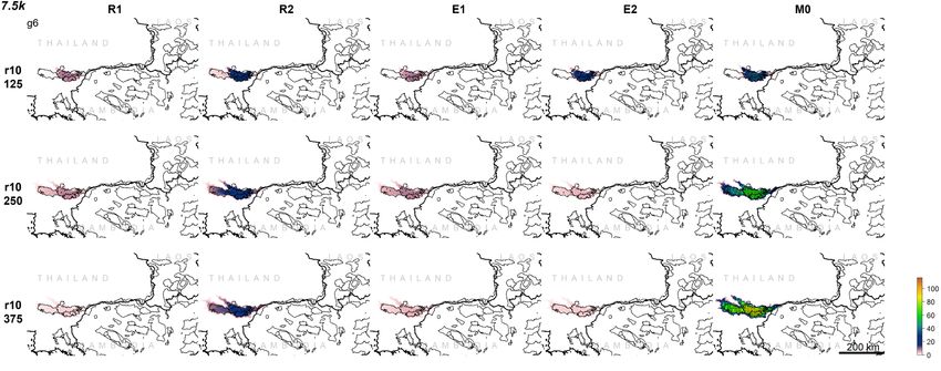
Land 2020, 9, 415                                                                                    2 of 27

through space and time in response to spatially varying habitat quality gradients, patterns of mortality
risk, and how landscape features drive movement and dispersal. Accounting for temporally dynamic
interactions among spatially explicit patterns of habitat quality, mortality rates and dispersal is a deeply
challenging task [5,6].
       Dispersal, range expansion, population viability, and other processes of research and management
interest emerge from complex interactions between a species’ life-history traits, landscape configuration,
and anthropogenic influence [7–9]. Researchers developing models of population dynamics in complex
landscapes face the challenging prospect of capturing these influential factors sufficiently to produce
reliable outputs. At a fundamental level, population dynamics are influenced considerably by landscape
heterogeneity at multiple scales and ecological patterns affecting biological processes, such as population
connectivity. Specifically, connectivity emerges as a function of the ability of organisms to move across
the landscape in response to three factors: distribution and density of the source population, resistance
of the landscape, and dispersal ability of the organism [10]. Perhaps most important, and usually
unaccounted for, spatially-heterogeneous mortality risk can dominate trajectories of population
dynamics through space and time [11,12]. To reliably predict population dynamics and connectivity,
it is therefore essential to integrate distribution, abundance, resistance, dispersal ability and mortality
risk explicitly into integrated spatial models (e.g., [5,6]).
       Variation in these parameters may drastically influence results. For example, a number of studies
have shown a high degree of sensitivity and complex interactions among factors affecting population
size, distribution and connectivity [5,6,9,12–15]. Empirical data necessary for accurate parameterization
of models may be difficult to obtain [16]. Thus, if researchers develop models via a narrowly or
vaguely-defined set of parameters, as is often the case [17], they may be limited in their ability to
ascertain if model predictions reflect what is likely to occur in reality. In addition, it is essential to
understand the relative sensitivity of models to variation in critical parameters, to assess how reliable
they are, given parametric uncertainty, and to guide on where empirical or theoretical research should
focus to improve the precision of parameter estimates.
       There are several key factors in the development of connectivity models used in spatially
explicit modeling of population dynamics that merit investigations into their effect. Such models are
often highly reliant on resistance surfaces, which define step-wise cost to movement and can aid in
determining paths for dispersal, and has received a high degree of focus (e.g., [16]). However, there has
been comparatively less attention on investigating the potential effect of non-linear relationships
between landscape configuration and cost to movement [9,18]. Importantly, while resistance surfaces
may implicitly incorporate mortality as a constraint to movement [19], they may be a poor correlate
for elevated mortality risk (e.g., hunting/poaching, road collisions, etc.) during dispersal, that can
otherwise drastically affect conclusions on functional connectivity in a landscape [11,20,21]. In reality,
mortality risk across landscapes can be highly spatially heterogeneous and models may not explicitly
incorporate or investigate its effects [12,22]. Predictions of landscape configuration and connectivity
can also be extremely sensitive to species dispersal ability or related parameters dictating movement
thresholds [23,24]. This reinforces the need for investigations into model sensitivity to dispersal ability,
particularly given that empirical movement data is rarely available to inform model development [16].
Lastly, investigations into the degree to which thresholds of population density or size interact with
these and other factors are less common than investigations into the effect of these factors on population
metrics [9,25].
       Simulation modeling has emerged as a critical investigation tool to understand and predict
spatially explicit population dynamics. Simulations can enable researchers to test hypotheses on the
effect of varying parameter values on predicted population distributions, abundance and landscape
connectivity [5,6,12,15]. However, somewhat neglected has been the use of simulations evaluating
temporal dynamics in a spatially explicit framework [26]. Incorporating time-sensitivity and temporal
dynamism in analysis enables evaluation of the degree of displacement from initial conditions through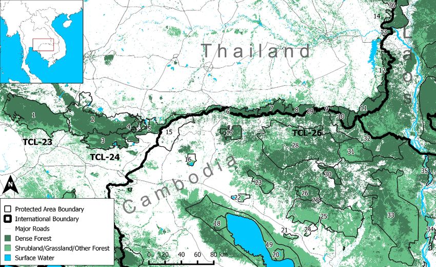
Land 2020, 9, 415 3 of 27
time, divergence between scenarios at each timestep, and time-lags in species response to landscape
configurations [26].
This study evaluates the degree to which simulations of population and connectivity dynamics in
a spatially explicit context are sensitive to the variation of critical parameters. Specifically, we apply a
dynamic spatial modeling approach, using cumulative resistance kernels [5,6] and spatially differential
mortality risk to test: (1) the strength of effects and interactions of parameters on predicted population
size, distribution and connectivity, and (2) the degree of displacement and divergence among
scenarios across timesteps. Concurrently, we evaluate the implications of these effects for the regional
conservation of an endangered species, the Indochinese tiger (Panthera tigris corbetti). We utilized
data from a population of tigers in the Dong Phayayen-Khao Yai forest complex (DPKY) in Eastern
Thailand [27]. We consider this to be an ideal candidate species since tigers are wide-ranging,
occur within metapopulations shaped considerably through dispersal and landscape configuration,
and are a species of notable and urgent conservation concern [28,29]. Tigers have suffered severe range
collapse throughout Southeast Asia, likely being extirpated from Cambodia, Laos, and Vietnam [30–32].
Our focal landscape of DPKY is likely to be the eastern-most breeding population of tigers in Southeast
Asia and may serve as a source population for recolonization of areas in which they were extirpated
both within and beyond this landscape. Understanding the population dynamics of this landscape,
its degree of connectivity with other potential habitats, and how these factors change over time will be
critical for developing long-term management and conservation strategies.
2. Materials and Methods
2.1. Study Area
Our study area (Figure 1) contains three tiger conservation landscapes (TCLs; [33]) with notable
protected area and forest coverage: the Dong Phayayen-Khao Yai Forest Complex in Eastern Thailand
(DPKY; TCLs-23/24), the Phnom-Dong Rak landscape in Eastern Thailand, and the Cambodian Northern
Plains (TCL-26) landscape in Northern Cambodia. DPKY is of particular importance, given it currently
supports an established breeding population of tigers (TCL-24; [27]) which could potentially disperse
to, and re-colonize, the other TCLs in which tigers have been extirpated (TCL-23/26). To account
for potential habitat which may facilitate tiger movement between and beyond these protected area
complexes, we generated a 45-km buffer from protected area borders in ArcGIS 10.3.1 (Environmental
Systems Research Incorporated, ESRI, Redlands, CA, USA, 2011). This distance was selected based on
the maximum scale of analysis considered in Reddy et al. [34] in their investigation of landscape-scale
gene flow of tigers in central India. This produced a total study area of ~157,920 km2 , including parts
of Thailand, Cambodia, and a small section of southern Lao PDR. The area contains a heterogeneous
mix of topography, forest, and anthropogenic land cover. Forest cover configuration in this area varies
considerably, from small, relatively isolated patches to large contiguous forest blocks. Much of this
forest cover occurs within protected areas, with most land use outside protected areas dominated by
agriculture, villages and urban areas.
2.2. Landscape Connectivity Simulations
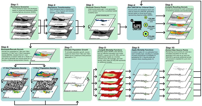
To test the sensitivity of landscape connectivity models, we varied four sets of factors: (1) resistance
surface ((i) highway mitigation scenario (SCEN); (ii) resistance transformation (RES)); (2) dispersal
ability (KERN); (3) population density (DENS); and (4) mortality function (MORT). Each factor set
included several levels to evaluate the influence of adjusting these factors on resulting simulated
population (N), cumulative resistance kernel extent (kernext), and kernel sum (kernsum), with kernels
generated from the Universal Corridor Network Simulator (UNICOR) v2.0 [38]. A workflow diagram
depicting these methods is presented in Figure 2.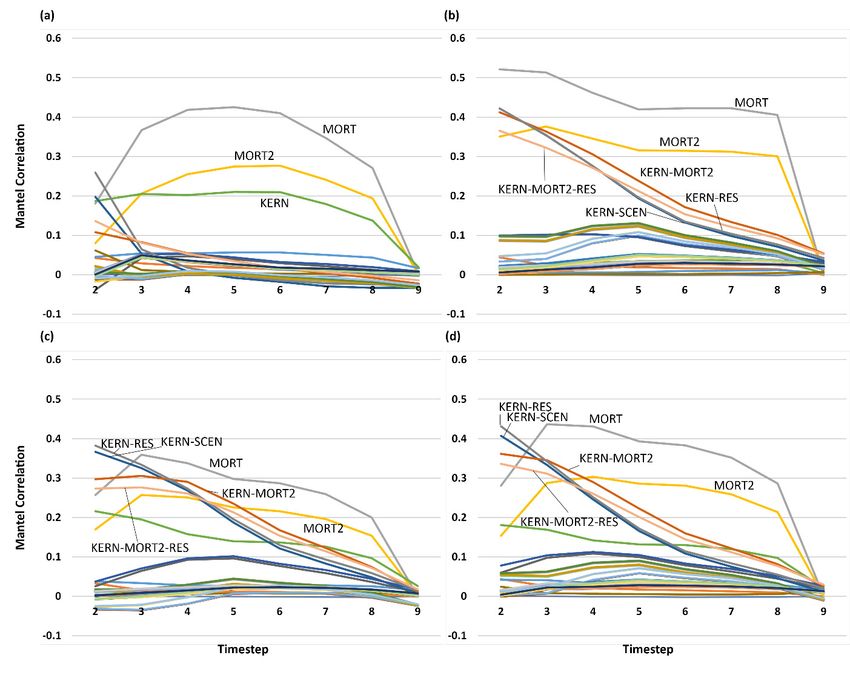
Land 2020, 9, 415                                                                                               4 of 27

Land 2020, 9, x FOR PEER REVIEW                                                                                            4 of 28

     Figure    1. Study
           Figure         area
                   1. Study      forfor
                              area    connectivity
                                         connectivityanalysis.
                                                       analysis. Protected  areaswere
                                                                 Protected areas  were   generated
                                                                                       generated    from
                                                                                                 from      UNEP-WCMC
                                                                                                      UNEP-WCMC
     and and
           IUCN    [35];[35];
                IUCN     a full   listing
                               a full       of names
                                       listing        cancan
                                               of names    be be
                                                               found
                                                                 foundinin
                                                                         Supplementary
                                                                           SupplementaryMaterials
                                                                                           Materials 1. Forest
                                                                                                         Forest cover
                                                                                                                cover was
          was generated
     generated     from 2018fromSERVIR–Mekong
                                    2018 SERVIR–Mekong       Regional
                                                         Regional      LandCover
                                                                     Land    Cover Monitoring
                                                                                   MonitoringSystem
                                                                                                 System(RLCMS;   [36])[36])
                                                                                                           (RLCMS;
           reclassed   into   dense    forest  (including  Forest,  Evergreen  Forest,  Flooded  Forest,
     reclassed into dense forest (including Forest, Evergreen Forest, Flooded Forest, and Mixed Forest),  and  Mixed
     and Forest),    and Shrubland/Grassland/Other
             Shrubland/Grassland/Other              Forest Forest  (including
                                                              (including       Shrubland, Grassland,
                                                                            Shrubland,     Grassland, Wetlands
                                                                                                         Wetlands and and
           Orchard/Plantation). Major roads were derived from OpenStreetMap [37]. The eastern section (TCL-24)
     Orchard/Plantation). Major roads were derived from OpenStreetMap [37]. The eastern section (TCL-
           of the Dong Phayayen-Khao Yai forest complex (2–5) acts as the source site for our simulations.
     24) of the Dong Phayayen-Khao Yai forest complex (2–5) acts as the source site for our simulations.
     2.2.1. Resistance Surfaces
2.2. Landscape Connectivity Simulations
           Our approach employs the use of resistance surfaces, a commonly-used foundation for applied
     connectivity
      To test theand        dispersal of
                        sensitivity    modeling
                                          landscape[17,39]. In resistancemodels,
                                                        connectivity      surfaces, wepixels in a landscape
                                                                                          varied    four setsareofassigned
                                                                                                                    factors: (1)
     values surface
resistance     reflecting ((i)step-wise
                                highwaycost   to individual
                                          mitigation    scenariomovement,
                                                                    (SCEN);with      low valuestransformation
                                                                               (ii) resistance     representing areas    of (2)
                                                                                                                     (RES));
     relatively   little  resistance  and high   values representing   strong   resistance.  Resistance
dispersal ability (KERN); (3) population density (DENS); and (4) mortality function (MORT). Each        surfaces   assume
     that landscape-level movement of organisms is dictated by cost of movement and that pixel values in
factor set included several levels to evaluate the influence of adjusting these factors on resulting
     the resistance surface accurately reflect that cost.
simulated population (N), cumulative resistance kernel extent (kernext), and kernel sum (kernsum),
           Resistance surfaces provide the foundation for connectivity analysis [16], but do not reflect
withconnectivity
       kernels generated           from theresistance
                       itself. Specifically,  Universal      Corridor
                                                         is point       Network
                                                                   specific,          Simulator
                                                                             but connectivity       (UNICOR)
                                                                                                is path or route v2.0   [38]. A
                                                                                                                   specific,
workflow
     governed diagram
                   by sourcedepicting   thesedistribution
                                 population    methods isand  presented
                                                                 density, in  Figure 2.
                                                                           resistance   of the landscape, and dispersal
     ability of the organism [10]. We employed resistant kernel modeling [40] to simulate the effects of
2.2.1.different
       Resistancelevels Surfaces
                           of dispersal ability, mortality, and resistance in predicting the dynamic spread of the
     tiger population over time. The resistant kernel method is particularly suitable for this application
      Our approach employs the use of resistance surfaces, a commonly-used foundation for applied
     given that it produces a spatial incidence function of the expected rate of movement through each cell
connectivity and dispersal modeling [17,39]. In resistance surfaces, pixels in a landscape are assigned
     in the landscape as a function of source population distribution, resistance and dispersal ability. Thus,
values    reflecting step-wise cost to individual movement, with low values representing areas of
     this is an ideal method for predicting rates and patterns of dispersal (e.g., [20]) and population spread
relatively   little resistance and high values representing strong resistance. Resistance surfaces assume
     (e.g., [5,6]).
that landscape-level movement of organisms is dictated by cost of movement and that pixel values
in the resistance surface accurately reflect that cost.
      Resistance surfaces provide the foundation for connectivity analysis [16], but do not reflect
connectivity itself. Specifically, resistance is point specific, but connectivity is path or route specific,
governed by source population distribution and density, resistance of the landscape, and dispersal
ability of the organism [10]. We employed resistant kernel modeling [40] to simulate the effects of
different levels of dispersal ability, mortality, and resistance in predicting the dynamic spread of the
tiger population over time. The resistant kernel method is particularly suitable for this application
given that it produces a spatial incidence function of the expected rate of movement through each
cell in the landscape as a function of source population distribution, resistance and dispersal ability.
Thus, this is an ideal method for predicting rates and patterns of dispersal (e.g., [20]) and population
Land 2020, 9, 415                                                                                                                                                              5 of 27
  Land 2020, 9, x FOR PEER REVIEW                                                                               5 of 28

       Figure
     Figure 2. 2.Diagram
                  Diagramdepicting
                            depictingmethods
                                      methodsworkflow,
                                               workflow,  including
                                                        including   development
                                                                  development  ofof highway
                                                                                  highway    crossing
                                                                                           crossing   resistance
                                                                                                    resistance   scenarios
                                                                                                               scenarios   (SCEN),
                                                                                                                         (SCEN),   resistance
                                                                                                                                 resistance    transformation
                                                                                                                                            transformation      (RES),
                                                                                                                                                              (RES),     adjusting
                                                                                                                                                                       adjusting
       dispersal
     dispersal    ability
                ability   (KERN),
                        (KERN),    adjusting
                                 adjusting   population
                                           population    density
                                                      density    (DENS),
                                                               (DENS),   and
                                                                       and   developing
                                                                           developing    and
                                                                                       and    applying
                                                                                           applying     mortality
                                                                                                     mortality    functions
                                                                                                                functions    (MORT).
                                                                                                                          (MORT).  AshAsh  et al.
                                                                                                                                        et al.    [41];
                                                                                                                                               [41];    Reddy
                                                                                                                                                     Reddy     et al.
                                                                                                                                                            et al.    [34].
                                                                                                                                                                   [34].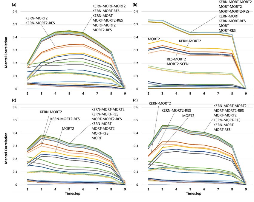
Land 2020, 9, 415                                                                                   6 of 27

     We tested potential resistance maps generated from Indian connectivity and tiger dispersal
models [34,41], an inversed locally-generated habitat suitability model [42], and an expert-derived
resistance surface (Supplementary Materials 1). Model predictions varied considerably. Empirical
models developed outside our study area either overpredicted resistance of relatively intact lowland
forest or overpredicted resistance along potentially important forest ridgelines likely to be used by
tigers [43,44]. Further, the inversed locally-generated habitat-suitability model [42] predicted unusually
high resistance in areas outside DPKY even in large areas of intact forest cover, potentially owing
to third order sampling for the model and a lack of representation of certain habitats occurring
outside this landscape. The expert model appeared to reflect patterns of likely tiger presence in DPKY
from the empirically-developed habitat-suitability model and predicted low resistance along forested
ridgelines and large blocks of forest, while appropriately scaling up resistance in human-dominated
areas. Expert-based approaches to parametrize resistance surfaces are often criticized as inaccurately
reflecting landscape effects on actual movement [16]. However, given the empirical models tested
did not reflect the particular context and limitations of our system and the expert-model reflected
behavioral patterns observed in the literature, the expert-derived resistance surface was identified as
the most suitable. Additional details can be found in Supplementary Materials 1.
     The expert-based approach utilized land cover data from the 2018 SERVIR–Mekong Regional
Land Cover Monitoring System (RLCMS; [36]). Land cover was reclassified into five resistance values:
Dense forest (1), Scrub forest (20), Agriculture-village matrix (50), Reservoirs/Surface Water (80),
and Urban areas (100). Minor and major roads [37] were assigned resistance values of 30 and 100,
respectively, where overlapping land-cover values were lower.
     Using this resistance layer, we developed three highway mitigation scenarios to test the effect of
highway crossing structures (SCEN). Scenarios included: S1—no mitigation of highways (resistance
layer as described above); S2—mitigation of local highway route 304 through wildlife crossing structures
with lower resistance (20) for pixels representing their present locations; and S3—mitigation of route
304 (S2) and hypothetical mitigation of another local highway, route 348. Further details can be found
in Supplementary Materials 1.
     To account for resistance uncertainty and evaluate sensitivity to resistance values, we further
modified resistance layers to test for three power functions (RES). In addition to the base resistance
layer (r10), we also calculated resistance layers to the 0.7 power (r07) and the 1.5 (r15) power which
were then rescaled from 1 to 100 and resampled to 250 m resolution. These functions transform the
linear shape of the resistance function of landcover into convex (0.7 power) or concave (1.5 power)
forms, reflecting different hypotheses about the relative resistance of landcover classes (e.g., [34]).

2.2.2. Population Source Points
     To simulate tiger dispersal from DPKY, we derived a set of source points, representing
individual animals, which were distributed probabilistically and proportional to tiger habitat suitability
(sensu [15,20]). First, we rescaled a multi-scale- and shape-optimized tiger habitat suitability model
developed by Ash et al. [41] for DPKY, in which values were proportional to predicted presence on a
scale from 0 to 1. Second, we calculated the difference between this layer and a uniform random raster
with values ranging from 0 to 1, extracting resulting pixels with positive values as potential source
points. Third, we drew a random sample of 30 points from these pixels, representing the upper range
of recent population estimates [45]. Source points were generated based on evidence that no tigers
currently occur in our study area outside of DPKY [30,32,46].

2.2.3. Dispersal Ability
     To evaluate potential dispersal from source points, we utilized UNICOR v2.0 [38] to generate
cumulative resistance kernels. These represent the sum of resistance kernels from each source point as a
function of total cost distance within the resistance layer and defined kernel width, reflecting predicted
density of dispersing individuals for each pixel [13,40]. We tested a range of dispersal abilities (KERN)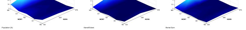
Land 2020, 9, 415                                                                                    7 of 27

by applying kernel widths of 125,000 (125 k), 250,000 (250 k), and 375,000 (375 k) cost-distance units (cu)
for each scenario (S1, S2, and S3) and resistance transformation (r7, r10, and r15). These kernel widths
correspond to potential dispersal distances of 125 km, 250 km, 375 km in ideal habitat (resistance value
of 1), respectively. While reliable dispersal data for tigers is rare, tigers are known to disperse within
this range of distances [47–49]. This enables evaluation of the effect of different dispersal abilities on
predicted connectivity (e.g., [13,20]) and population spread [6].

2.2.4. Population Density and Growth
      We used a dynamic kernel spread modeling approach first described by Cushman [5] and recently
applied in a similar way in Barros et al. [6] which models changes in population distribution across
a temporally dynamic framework. Specifically, we modeled population spread across nine discrete
timesteps, representing non-overlapping generations. At each timestep, new source points were
generated based on kernel layers generated by UNICOR in the previous timestep. To test for the effects
of different densities of the tiger population (DENS, e.g., area-specific carrying capacity) these source
points were generated at one of two maximum densities. For each factor combination, kernel surfaces
were resampled by bilinear interpolation either to 7500 m (7.5 km) or 10,000 m (10 km) resolution.
This resulted in two different densities of source points (maximum of 1/56.26 km2 or 1/100 km2 ),
reflecting potential differences in simulated territory spacing and carrying capacity of tigers in the study
area. These resampled kernel layers were rescaled between 0 and 1, which was then subtracted by a
uniform random raster (0–1). This difference raster produced a probabilistic layer for the generation of
new source points at both densities for the next timestep, proportional to predicted dispersal density.
      To determine the number of source points generated at each timestep and to evaluate simulated
population spread, we used a maximum population growth rate of 1.5 per generation timestep
(previous generation × 1.5). This assumes half a given population are breeding females with a relatively
conservative mean lifetime fecundity of three (see [50–52]). These source points were then used as
an input to run UNICOR for the next generational timestep. This was repeated for each subsequent
timestep (up to 9). In effect, the population (N) and distribution of source points for each timestep and
factor combination were based on probabilistic sampling of kernels at one of two densities, a maximum
potential population growth rate of 50% per timestep, and random chance.

2.2.5. Mortality
     To investigate the potential effect of mortality on the simulated population (MORT), at each
timestep we filtered source points based on one of five mortality functions, representing spatially
differential probability of survival (pixel values ranging 0 to 1).
     Function M0 represents the base scenario described above wherein source points for each timestep
were determined by a combination of kernel density, maximum potential population growth rate,
and random chance, with no additional modifications.
     Functions R1 and R2 were based on a tiger effective population size model from Reddy et al. [34],
applied with locally generated spatial layers to predict the potential effective population size of
tigers in our study area. The model predicts tiger effective population size as a function of the focal
mean of protected area coverage within a 45-km radius, mean forest cover within a 45-km radius,
and mean landscape resistance within a 42.5 km radius. In contrast to the resistance model derived
from Reddy et al. [34] which defined resistance via specific habitat patterns not reflected in our
study landscape, the effective population size model parsimoniously generated predictions broadly
applicable to tigers throughout their range (i.e., broad extents of forest cover and protected area
presence) [31,53–55]. This model produced predictions reflecting reasonable and consistent patterns
of high and low potential presence, and by extension, potential survivability across our landscape.
This model, rescaled between 0 and 1, was used to predict mortality risk (R1), representing high
mortality risk where predicted potential effective population size is low.
Land 2020, 9, 415                                                                                    8 of 27

      To account for uncertainty and investigate the sensitivity of simulations to variation in spatial
mortality risk, we calculated the square root of R1, reducing mortality risk in moderate to high
suitability areas (R2).
      For comparison of approaches and to further test model sensitivity, we also tested two additional
expert-based mortality functions with spatially differential probability of mortality (E1 and E2).
Evidence suggests that survival probability of dispersing tigers, particularly outside protected areas,
can be moderately to extremely low [56,57]. To account for this, we generated a simplified spatially
differential mortality risk layer in which survival is a function of available tree cover, protected area
coverage, and presence of roads. This layer of spatial probability of survival was capped at 0.8 in
protected areas with 100% forest cover and no roads within a 20 km radius, declining in probability as
forest cover decrease and road density within 20 km increase, lower by a factor of 10 outside protected
areas. To account for uncertainty and to test the sensitivity of results to this mortality function, we also
produced a modified expert-derived survivability scenario (E2) following the approach of E1 but
modifying the maximum survivability outside protected areas from 10% to 50%. Formulas for these
functions are depicted in Supplementary Materials 1.
      Mortality functions were applied following the generation of source points for each timestep
and parameter combination. At each timestep, mortality layers (values representing low (0) to high
(1) probability of survival) were subtracted by a random raster with values from 0 to 1. Source points
overlapping with pixels in the difference raster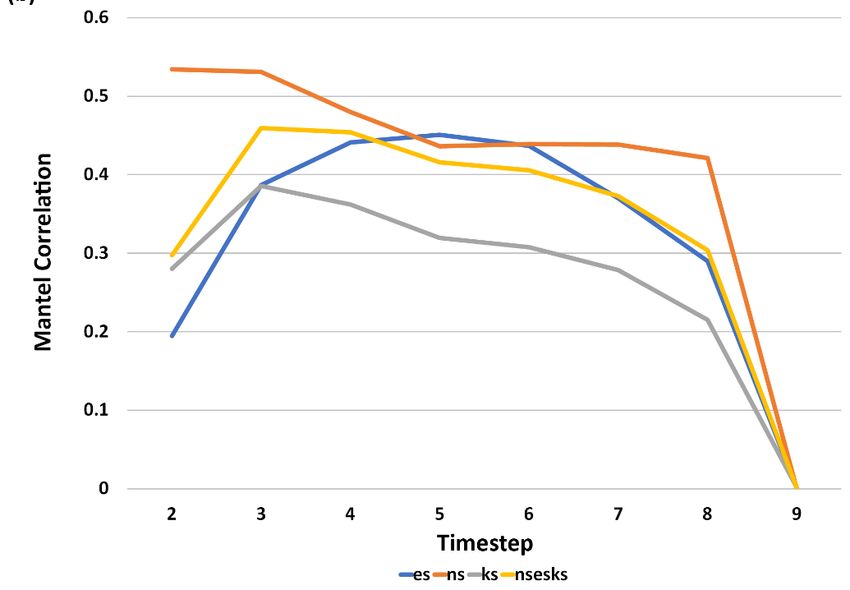
Land 2020, 9, 415                                                                                   9 of 27

      To test for significant differences between N, kernel extent, and kernel sum across the four
investigated factors—resistance surface (SCEN and RES), dispersal ability (KERN), population density
(DENS), and mortality function (MORT)—we conducted a factorial analysis of variance (ANOVA),
considering differences significant if p < 0.05. To investigate the strength and form of multivariate
interactions, we produced time-series maps, surface plots via Matlab (version 18c, MathWorks, Inc.,
Natick, MA, USA), and multivariate trajectory analysis [26], plotting predicted connectivity values
across the nine timesteps/generations for the mean of all replications for each combination of factors.
We used Mantel tests [58] to evaluate the effect size and interactions among factors. We evaluated two
distance-based response variables, divergence among scenarios, and displacement of scenarios from
initial conditions [26]. The Mantel analysis quantifies the effect size (as measured by Mantel r value)
of the correlation between the response (divergence or displacement) and whether scenarios had the
same or different levels of each factor (SCEN, RES, KERN, DENS, and MORT).

3. Results
     Our simulations produced clear and significant differences in simulated population size, kernel
extent, and kernel sum trajectories with evidence of strong interactions among factors. These factors
drive varying degrees of divergence and displacement from initial states, with implications for patterns
of dispersal, colonization, and population persistence. We describe these results in detail below.

3.1. Population Trajectory and Colonization
      The majority of simulations (~73%; 1965), by timestep 9, had population values lower than the
baseline (N = 30; Table 1; Supplementary Materials 2, Table S1). In simulations where population values
increased, 72% (507) were those with no additional mortality (M0) and higher population density
(7.5 km—62% of runs where N > 30). Conversely, population declines were associated primarily
with elevated spatially differential mortality functions with little difference among population density,
resistance transformation, or dispersal ability. However, the frequency of extinction (population
declines to 0 by timestep 9) increased with resistance transformation from concave to convex (19% to
49% of extinctions) and higher dispersal ability (2% of simulated extinctions were with a dispersal
ability of 125 kcu, up to 74% with a dispersal ability of 375 kcu).
      A large majority of simulations (93%, 2510) resulted in dispersal to KYNP in at least one timestep.
However, colonization of KYNP (presence at timestep 9) was considerably lower (53%, 1425; Table 1;
Supplementary Materials 2, Table S2). Simulations tended to have a lower frequency of dispersal to
KYNP when dispersal ability was lower (79% (712) of simulations with dispersal ability of 125 kcu
vs. 100% for 250 kcu and 375 kcu simulations), with much lower rates of successful colonization
(41% (371) for 125 kcu, 68% (609) for 250 kcu, and 49% (445) for 375 kcu). Dispersal to this area was also
slightly lower for simulations with concave resistance (85% (765) of r07 simulations vs. 95% and 99%
for r10 and r15, respectively), and those with larger territory spacing (90% (1217) in simulations with
10 km spacing vs. 96% (1293) with 7.5 km spacing). These trends also hold when considering rates of
successful colonization with varying resistance (49% (438) of r07 simulations, 53% (473) of r10 and 57%
(514) of r15). Approximately 20% (547) of all simulations resulted in dispersal to areas in Cambodia in
at least one timestep, largely attributed to scenarios with no additional mortality (78% (425) instances).
Successful colonization of areas in Cambodia was only observed in 9% (243) of simulations, of which
97% (235) were in scenarios with no additional mortality (M0). There was generally a higher rate of
dispersal to and colonization of areas in Cambodia as resistance shifted from concave (r07) to convex
(r15) forms and as dispersal ability increased (125 kcu to 375 kcu). Only 2% (41) of simulations resulted
in dispersal to Laos in any timestep, with only 1% (38) of simulations resulting in colonization. All of
these cases were in simulations with no additional mortality (M0) and maximum dispersal ability
(375 kcu), with almost all cases when resistance was convex (r15). Dispersal to and colonization of areas
outside the source site did not appear substantially affected by highway mitigation scenario (SCEN).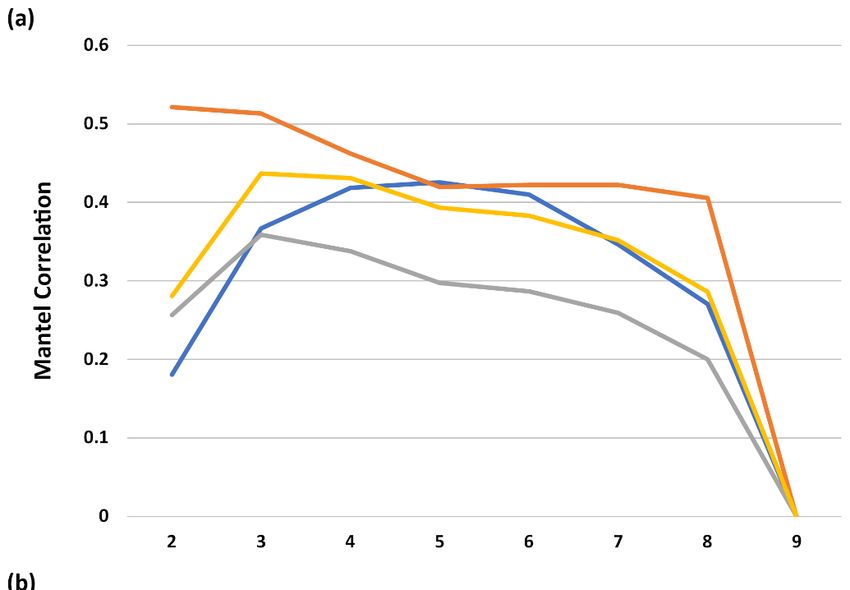
Land 2020, 9, 415                                                                                           10 of 27

      Table 1. Summary of simulation results within factor groups by parameter at timestep 9 out of
      2700 simulations. Results are summarized by (a) simulated population (N) at timestep 9 and (b) number
      of simulations in which source points were generated in Khao Yai National Park (NP), Cambodia,
      or Laos at timestep 9 (e.g., successful colonization). This reflects a summary of all simulation results
      specific to each factor group—resistance surface (highway mitigation scenario (SCEN) and resistance
      transformation, (RES)), dispersal ability (KERN), population density (DENS), and mortality function
      (MORT)—amalgamating all other factors and parameters. A detailed breakdown of simulation results
      can be found in Supplementary Materials 2; Tables S1 and S2.

                                                 (a)                                       (b)
     Factor     Parameter
                              N > 30    N = 30     N = 1 to 30   N=0      Khao Yai NP      Cambodia      Laos
     SCEN             S1       233          7          500         160         455               79       16
                      S2       238         11          508         143         498               76        9
                      S3       235         11          499         155         472               88       13
     DENS           10 km      268         18          812         252         641               99       18
                    7.5 km     438         11          695         206         784               144      20
    MORT             M0        507         5            28          -          474               235      38
                     E1         4          3           363         170         169                1        -
                     E2        21          5           393         121         220                1        -
                     R1         -           -          373         167         124                -        -
                     R2        174         16          350          -          438                6        -
      RES             r07      243         17          555          85         438                64       -
                      r10      240         5           508         147         473                69       1
                      r15      223         7           444         226         514               110      37
     KERN           125 kcu    264         17          608          11         371                12       -
                    250 kcu    256         10          525         109         609                92       -
                    375 kcu    186          2          374         338         445               139      38
                      All      706         29          1507        458         1425              243      38

3.2. Analysis of Variance
     The factorial analysis of variance of the effects of factors on predicted population size (N),
extent of connected population (kernext), and sum of kernel density (kernsum) showed clear and
consistent patterns across all three response variables. All main effects, with the exception of highway
mitigation scenario (SCEN) and resistance transformation (RES; N at timestep 4)), were very highly
significant across timesteps for all three response variables (Supplementary Materials 2, Tables
S3–S29). In contrast, SCEN was only significant for timesteps 2–5 for kernsum. Two-way interactions
of population density with mortality function (DENS:MORT), mortality function with resistance
transformation (MORT:RES), and mortality function with dispersal ability (MORT:KERN) were very
highly significant for all timesteps for all three response variables. Two-way interactions of highway
mitigation scenario and mortality (SCEN:MORT) were significant for timesteps 2–6 for kernsum and
timesteps 5–7 for N. Among three-way interactions, DENS:MORT:KERN was significant in all timesteps
across response variables, MORT:RES:KERN was significant for all timesteps and response variables
with the exception of two timesteps for N, and DENS:RES:KERN was significant in 75% of time steps
for all response variables. The three-way interaction DENS:MORT:RES was significant in 88% of
timesteps for N and kernsum, but only 50% of timesteps for kernext. Three-way interactions involving
SCEN (SCEN:MORT:RES and SCEN:MORT:KERN) were only significant at timestep 5 for kernsum.
None of the other three-way interactions were significant for any timestep for any response variable.
The four-way interaction of DENS:MORT:RES:KERN was significant across 75% of timesteps for N, 88%
of timesteps for kernsum, and 50% for kernext, and the four-way interaction of SCEN:DENS:MORT:RES
was only significant at timestep 3.
Land 2020, 9, 415 11 of 27
The ANOVA results underscore two main outcomes. First, there are strong multivariate interactions,
particularly between dispersal ability (KERN), resistance transformation (RES), mortality function
(MORT), and territory spacing (DENS). Second, highway mitigation scenario (SCEN) and its interactions
did not affect response variables as significantly compared to other factors in our modeling experiment.
Given it is difficult to interpret the main effects in the presence of strong interactions, further analysis
focused on deconstructing these interactions.
3.3. Multivariate Interactions
Time-series maps (Figure 3; Supplementary Materials 3, Figures S1–S6) and surface plots (Figure 4;
Supplementary Materials 3, Figures S7–S12) demonstrated a number of strong interactions between
factors. First, mortality function interacts strongly with dispersal ability. In the absence of spatially
elevated mortality risk (M0), all three response variables increase dramatically at later timesteps,
particularly for simulations with greater dispersal ability and higher potential population density
(7.5 km). In contrast, simulations with elevated mortality risk (R1, R2, E1, and E2) show no large
increase in any of the three response variables across timesteps, and, in simulations with the highest
dispersal ability (375 kcu), populations frequently declined to extinction as a result of dispersal
mortality exceeding replacement.
Generally, N and kernsum values increased in simulations with higher maximum potential tiger
density (7.5 km), especially in scenarios with higher dispersal and (relatively) lower mortality risk.
Kernext increases are greatest in scenarios with low mortality, high dispersal, and lower maximum
potential tiger density, as this forces the population to spread more rapidly across a greater extent as
available territories fill faster at lower density. The different resistance scenarios interact with mortality,
density and dispersal such that N and kernsum variables greatly increase, especially in later timesteps.
This is the case when there is low mortality risk, high dispersal, high potential maximum density,
and when resistance is convex and does not highly penalize marginal habitat. In this combination of
parameters, the rate of population growth is maximized.
3.4. Multivariate Trajectory Analysis
Multivariate trajectory analysis plots (Figure 5; Supplementary Materials 3, Figures S13–S18), show
trajectories over time of simulations corresponding to all combinations of dispersal ability, territory
density, resistance transformation, and mortality scenario in a three-dimensional space defined by
kernext, kernsum and N. These trajectories show that the major differences are related to mortality risk
(MORT) interacting with dispersal ability (KERN), with additional, but lesser effects, from resistance
transformation (RES) and population density (DENS). Specifically, most scenarios that have elevated
mortality risk as an inverse function of habitat quality do not result in large increases in any of the three
connectivity measures (kernext, kernsum or N) over the simulated time frame. In contrast, scenarios
in which there is no elevated mortality risk (red spheres in Figure 5) show large increases over time,
especially for scenarios in which population density is higher (up to 1/7.5 km2 ), with substantially
lesser effects for different resistance surfaces. Figure 5 shows one view of this three-dimensional space
at timestep 6 and readers are encouraged to view the full 3D dynamic visualizations in Supplementary
Materials 3.Land 2020, 9, 415 12 of 27
Land 2020, 9, x FOR PEER REVIEW 12 of 28
Figure 3. Sample
Figure maps
3. Sample demonstrating
maps demonstrating divergence
divergencein cumulative resistance
in cumulative kernels
resistance andand
kernels populations between
populations combinations
between combinationsof mortality function
of mortality (MORT—R1,
function (MORT—R1, R2, R2,
E1, E2,
andE1,
M0)E2,and
anddispersal
M0) andability (KERN—125
dispersal kcu, 250 kcu,
ability (KERN—125 and250
kcu, 375kcu,
kcu)and
at timestep
375 kcu) 6,
atholding
timestephighway mitigation
6, holding highwayscenario (SCEN—S3),
mitigation territory spacing
scenario (SCEN—S3), (DENS—7.5
territory spacingkm),
and(DENS—7.5
resistance transformation (RES—r10)
km), and resistance constant.(RES—r10)
transformation Values reflect the expected
constant. cumulative
Values reflect densitycumulative
the expected of dispersing individuals
density from each
of dispersing source point.
individuals Additional
from each source maps
point.and
Additional
timestep maps and
animations can timestep
be foundanimations can be found
in Supplementary in Supplementary
Materials 3, Tables S1–S6.Materials 3, Tables S1–S6.Land 2020, 9, 415 13 of 27
Land 2020, 9, x FOR PEER REVIEW 13 of 28
(a) (b) (c)
Figure
Figure4. 4.
Surface
Surface plots
plotsshowing
showingvariation
variationininpredicted
predicted (a)
(a) population size (N),
population size (N),(b)
(b)kernel
kernelextent,
extent,and
and(c)(c) sum
sum of of kernel
kernel value
value for for
the the 15 combinations
15 combinations of dispersal
of dispersal ability
ability
(KERN—3
(KERN—3 levels) and
levels) andmortality
mortality risk (MORT—5
risk (MORT—5levels)levels)for
forresistance
resistancetransformation
transformation1.0 1.0(RES—r10)
(RES—r10)and andmaximum
maximum density
density 1/7.5
1/7.5 km
km (DENS—7.5
2
2 (DENS—7.5 km) km) atat timestep 9. The
timestep 9.
figure shows shows
The figure a strong interaction
a strong between
interaction dispersal
between abilityability
dispersal and mortality risk, with
and mortality risk,the
withpredicted valuesvalues
the predicted of all three variables
of all three remaining
variables low for
remaining lowallfor
scenarios involving
all scenarios
elevated mortality
involving elevatedrisk, across all
mortality dispersal
risk, abilities,
across all dispersalwhile all three
abilities, variables
while increase
all three linearly
variables with
increase dispersal
linearly withability when
dispersal therewhen
ability is no there
differential mortality risk
is no differential across the
mortality
landscape. Animations of these and other plots can be viewed in Supplementary Materials 3, Tables S7–S12.
risk across the landscape. Animations of these and other plots can be viewed in Supplementary Materials 3, Tables S7–S12.Land 2020, 9, 415 14 of 27
Land 2020, 9, x FOR PEER REVIEW 14 of 28
Figure
Figure 5. Three
5. Three orthogonal
orthogonal views
views of the
of the three-dimensional
three-dimensional trajectory
trajectory of of scenarios
scenarios in in a space
a space defined
defined by
by kernel extent, sum kernel value, and population size, at timestep 6 across density (DENS)
kernel extent, sum kernel value, and population size, at timestep 6 across density (DENS) and resistance and
resistance transformations
transformations (RES). Sphere(RES).
color Sphere
indicatescolor indicates
different different combinations
combinations of dispersal
of dispersal ability (KERN)ability
and
(KERN) and mortality risk (MORT). The figure shows that scenarios with low mortality
mortality risk (MORT). The figure shows that scenarios with low mortality risk (M0; red spheres) risk (M0; redin
spheres) in which population density is high have much greater predicted kernel extent, kernel sum,
which population density is high have much greater predicted kernel extent, kernel sum, and higher
and higher simulated population size (extreme values extending outside axis limits). Animations of
simulated population size (extreme values extending outside axis limits). Animations of these and
these and other plots can be viewed in Supplementary Materials 3, Tables S13–S18.
other plots can be viewed in Supplementary Materials 3, Tables S13–S18.Land 2020, 9, x FOR PEER REVIEW 15 of 28
3.5. Analysis of Effect Size and Interactions among Factors Using Mantel Tests
The full table of all Mantel results sorted by effect size is shown in Supplementary Materials 2
Land 2020, 9,S30–S37)
(Tables 415 15 of 27
for divergence and displacement, respectively. The main results are most easily
presented as line graphs (Figures 6 and 7). For divergence of scenarios from each other over time,
mortality function (MORT) had the dominant effect. For each response variable (kernext, kernsum, N
3.5. Analysis
and of Effect Sizecombination
the multivariate and Interactions amongthe
of these) Factors Using model
mortality Mantelmatrix
Tests in which all mortality
scenarios
The fullaretable
coded ofasall
1 and the non-mortality
Mantel results sorted scenarios
by effectas size
0 wasismost
shownsupported across all timesteps,
in Supplementary Materials
followed by the ordinal mortality model in which scenarios were
2 (Tables S30–S37) for divergence and displacement, respectively. The main results ordered from lowest tomost
are highest
easily
mortality risk (MORT2). Dispersal ability (KERN) and the interaction of dispersal
presented as line graphs (Figures 6 and 7). For divergence of scenarios from each other over time, distance and
ordinal mortality (KERN-MORT2) had moderate relative effect size, which was nearly equal to
mortality function (MORT) had the dominant effect. For each response variable (kernext, kernsum,
mortality in the first few timesteps but dropped to low relative support, comparatively, in later
N and the multivariate combination of these) the mortality model matrix in which all mortality
timesteps (Figure 6). For displacement of response variable values from initial condition, there was a
scenarios are coded as 1 and the non-mortality scenarios as 0 was most supported across all timesteps,
different, but even clearer pattern (Figure 7). For all response variables (kernext, kernsum, N and the
followed by the ordinal mortality model in which scenarios were ordered from lowest to highest
multivariate combination of these), the interaction between dispersal ability (KERN) and mortality
mortality
(MORT riskand(MORT2).
MORT2) had Dispersal abilityMantel
the highest (KERN) and the interaction
correlation across all of dispersalThere
timesteps. distance
wasand ordinal
similar
mortality (KERN-MORT2)
support for mortality effectshad moderate
alone (MORT),relative effect interacting
and mortality size, which wasresistance
with nearly equal to mortality
transformation
in (MORT-RES).
the first few timesteps but dropped to low relative support, comparatively, in later timesteps
(FigureThere
6). For displacement
were of responsein
consistent relationships variable
terms ofvalues from effect
the relative initialsize
condition, there wasbetween
of the correlation a different,
butthe
even
bestclearer
modelpattern
and the(Figure 7). For all
four response response
variables variables
over timesteps (Figurekernsum,
(kernext, 8). AcrossN and the multivariate
all timesteps, the
combination
best Mantelofmodel
these),hadthe the
interaction between dispersal
largest correlation ability (KERN)
with predicted and by
N, followed mortality
kernext (MORT
and theand
multivariate
MORT2) combination
had the of the three
highest Mantel responseacross
correlation variables. Kernsum hadThere
all timesteps. the lowest correlation
was similar with for
support
divergence
mortality or displacement
effects alone (MORT), across
andall timesteps.
mortality interacting with resistance transformation (MORT-RES).
Figure6.6. Mantel
Figure correlationsbetween
Mantel correlations betweenresponse
response variables
variables (a) Kernel
(a) Kernel Extent,
Extent, (b) Population
(b) Population Size, (c)Size,
(c)Kernel
KernelSum,
Sum,and
and(d)
(d)multivariate
multivariate distance between these response variables and divergence
distance between these response variables and divergence among among
scenarios
scenariosover
overtimesteps. Timestepis is
timesteps. Timestep depicted
depicted on the
on the x-axis
x-axis with with Mantel
Mantel correlation
correlation on theThe
on the y-axis. y-axis.
The highest correlating factors are labeled: MORT—mortality model matrix with all mortality scenarios
coded 1 and non-mortality 0; MORT2—mortality model matrix with scenarios coded ordinally from
highest to lowest degree of mortality risk; KERN—dispersal distance varying with kernel bandwidth;
KERN-MORT2—model matrix combining KERN and MORT2 by addition; KERN-RES—model matrix
combining KERN and resistance model matrices by addition; KERN-SCEN—model matrix combining
KERN and highway mitigation model matrices by addition; and KERN-MORT2-RES—model matrix
combining KERN, MORT2 and RES model matrices by addition.coded 1 and non-mortality 0; MORT2—mortality model matrix with scenarios coded ordinally from
highest to lowest degree of mortality risk; KERN—dispersal distance varying with kernel bandwidth;
KERN-MORT2—model matrix combining KERN and MORT2 by addition; KERN-RES—model
matrix combining KERN and resistance model matrices by addition; KERN-SCEN—model matrix
Landcombining
2020, 9, 415 KERN and highway mitigation model matrices by addition; and KERN-MORT2-RES— 16 of 27
model matrix combining KERN, MORT2 and RES model matrices by addition.
Figure 7. Mantel correlations between response variables (a) Kernel Extent, (b) Population Size,
Figure 7. Mantel correlations between response variables (a) Kernel Extent, (b) Population Size, (c)
(c) Kernel Sum, and (d) multivariate distance between these response variables and displacement
Kernel Sum, and (d) multivariate distance between these response variables and displacement of
of scenarios from initial value over timesteps. Timestep is depicted on the x-axis with Mantel
scenarios from initial value over timesteps. Timestep is depicted on the x-axis with Mantel correlation
correlation on the y-axis. The highest correlating factors are labeled: MORT—mortality model matrix
on the y-axis. The highest correlating factors are labeled: MORT—mortality model matrix with all
with all mortality scenarios coded 1 and non-mortality 0; MORT2—mortality model matrix with
mortality scenarios coded 1 and non-mortality 0; MORT2—mortality model matrix with scenarios
scenarios coded ordinally from highest to lowest degree of mortality risk; KERN—dispersal distance
coded ordinally from highest to lowest degree of mortality risk; KERN—dispersal distance varying
varying with kernel bandwidth; KERN-MORT2—model matrix combining KERN and MORT2 by
with kernel KERN-RES—model
addition; bandwidth; KERN-MORT2—model
matrix combiningmatrix
KERNcombining KERN
and resistance andmatrices
model MORT2 byby addition;
addition;
KERN-RES—model matrix combining KERN and resistance model matrices by addition;
MORT2-SCEN—model matrix combining MORT2 and highway mitigation model matrices by addition MORT2-
SCEN—model matrix combining MORT2 and highway mitigation model matrices by
and KERN-MORT2-RES—model matrix combining KERN, MORT2 and RES model matrices by addition.addition and
KERN-MORT2-RES—model matrix combining KERN, MORT2 and RES model matrices by addition.
There were consistent relationships in terms of the relative effect size of the correlation between
the best model and the four response variables over timesteps (Figure 8). Across all timesteps, the best
Mantel model had the largest correlation with predicted N, followed by kernext and the multivariate
combination of the three response variables. Kernsum had the lowest correlation with divergence or
displacement across all timesteps.Land 2020, 9, 415 17 of 27
Land 2020, 9, x FOR PEER REVIEW 17 of 28
Figure
Figure 8.
8. Plot
Plot of
of Mantel
Mantel correlation
correlation of
of the
the best
best model
model for
for (a)
(a) divergence
divergence and
and (b) displacement over
(b) displacement over
timesteps
timesteps for each of the response variables: es—kernel extent, ns—population size, ks—kernel
for each of the response variables: es—kernel extent, ns—population size, ks—kernel sum,
sum,
and
and nsesks—multivariate
nsesks—multivariate combination
combination of of kernel
kernel extent,
extent, population
population size, and kernel
size, and kernel sum.
sum. In
In both
both
cases,
cases, population size had
population size had the
thestrongest
strongestcorrelation
correlationwith
withthe
thebest
best scenario
scenario model
model matrix
matrix over
over nearly
nearly all
all timesteps,
timesteps, only
only equaled
equaled by by kernel
kernel extent
extent in timestep
in timestep 5. 5.
4. Discussion
4. Discussion
The ability
The ability of
of models
models toto produce
produce reliable
reliable and
and meaningful
meaningful predictions
predictions ofof population
population distribution,
distribution,
abundance and connectivity is governed by the interactive and temporally dynamic
abundance and connectivity is governed by the interactive and temporally dynamic effects of effects of several
several
factors such as landscape resistance, population density, dispersal ability, and mortality. Using aa
factors such as landscape resistance, population density, dispersal ability, and mortality. Using
spatially and
spatially and temporally
temporally explicit
explicitsimulation
simulationapproach,
approach,we weinvestigated
investigatedthethe
impacts of of
impacts these factors
these on
factors
on population connectivity and population size of tigers in Eastern Thailand. Our studya
population connectivity and population size of tigers in Eastern Thailand. Our study demonstrated
high degree ofasensitivity
demonstrated high degreeof simulated population
of sensitivity size, extent
of simulated and connectivity
population size, extent to parameter
and values
connectivity to
and, in particular,
parameter values evidence of strong interactions
and, in particular, evidence of between
strong factors which between
interactions may drastically
factors affect
which results.
may
Dispersal ability
drastically affect and spatially
results. differential
Dispersal mortality
ability risk dominated
and spatially predictions
differential of connectivity
mortality risk dominated and
predictions of connectivity and population size, and these factors strongly interacted to affect
predictions. While similar dominant effects of dispersal ability on connectivity predictions wereLand 2020, 9, 415 18 of 27
population size, and these factors strongly interacted to affect predictions. While similar dominant
effects of dispersal ability on connectivity predictions were previously reported by several studies
(e.g., [9,10,20]), less attention has been directed to the effect of spatially differential mortality risk on
population size and connectivity [11,12,15].
This is among the first studies to explicitly evaluate the interaction of dispersal ability and
mortality on population size, distribution and connectivity in a spatially and temporally explicit
dynamic framework. Distribution and density of individuals in the population had intermediate effects
on predictions, landscape resistance overall had relatively low impacts on predicted connectivity,
and small-scale mitigation of linear barriers had limited measurable impact. Importantly, there was a
high degree of variation in the relative importance of factors depending on whether the assessment was
based on divergence among scenarios or displacement of scenarios from initial conditions. Furthermore,
results differed depending on whether the assessment was based on extent of connected kernel, sum of
kernel value, or population size. Our study also documented temporal variation in the relative effects
of different factors on connectivity. These results are of particular relevance to the development of
connectivity and species dispersal modeling and for conservation planning. We elaborate and discuss
each of these main results in the paragraphs that follow.
First, for both displacement (change of a single scenario from initial condition) and divergence
(difference between scenarios at a given timestep) of scenarios, we found that spatially heterogeneous
mortality risk and dispersal ability dominated predictions of connectivity and population size.
Main effects for these factors had very highly significant differences in population and connectivity
metrics across all timesteps and exhibited the strongest effects when comparing Mantel correlations.
Spatially heterogeneous mortality risk is frequently not accounted for in dispersal and population
connectivity modeling studies [12,22], despite evidence that dispersal or hostile matrix-related
mortality can exert a considerable influence on species populations and lead to greater vulnerability to
demographic stochasticity [59–61]. Resistance surfaces, which are widely used, may indirectly account
for mortality as a function of a more generalized resistance to dispersal [9,12,15,16,19], though this
relationship may be tenuous and lack transparency. Its entanglement with other factors affecting
distribution and movement precludes the ability to discern how mortality influences connectivity via
realized dispersal, potentially leading to overestimates of the degree of connectivity within a landscape
from the perspective of the organism in question [19]. Our results suggest that the application of an
additional function of mortality in connectivity modeling can produce highly divergent conclusions on
the degree of connectivity within a landscape and trajectory of the population of study. These results
are similar to the findings of Kaszta et al. [12] and Kramer-Schadt et al. [11] in which the introduction
of mortality risk via infrastructure resulted in isolation and declines of populations of wide-ranging
felids that would have otherwise been predicted to be highly connected based on habitat quality and
resistance alone.
Similarly, our results were particularly sensitive to dispersal ability, which exerted a relatively
disproportionate effect on population and connectivity trajectories. This is consistent with a
number of other studies in which predictions of landscape configuration and connectivity were
extremely sensitive to parameters associated with dispersal ability or related parameters dictating
movement thresholds [23,24]. While some models may be relatively insensitive to dispersal ability [62],
this nonetheless underscores the need for particular care in developing these parameters. Ideally,
dispersal models should be parameterized with reliable, empirically-derived movement data,
though this can be considerably difficult to obtain and are rarely applied in dispersal modeling
studies [16,21,28]. This presents a particular challenge to those investigating landscape connectivity
where the dispersal ability of target species is poorly understood. Studies in which the latter situation
applies may benefit from testing a range of dispersal ability values to account for this uncertainty and
potential sensitivity in such parameters.
Second, dispersal ability and mortality risk strongly interacted to affect connectivity predictions,
with very high predicted connectivity and population size when dispersal ability is high and mortalityYou can also read