An Incompressible Smoothed Particle Hydrodynamics (ISPH) Model of Direct Laser Interference Patterning - MDPI
←
→
Page content transcription
If your browser does not render page correctly, please read the page content below
computation
Article
An Incompressible Smoothed Particle Hydrodynamics
(ISPH) Model of Direct Laser Interference Patterning
Cornelius Demuth 1 and Andrés Fabián Lasagni 1,2, *
 1   Institute of Manufacturing Technology, Technische Universität Dresden, P.O. Box, 01062 Dresden, Germany;
     cornelius.demuth@iwtt.tu-freiberg.de
 2   Fraunhofer Institute for Material and Beam Technology IWS, Winterbergstraße 28, 01277 Dresden, Germany
 *   Correspondence: andres_fabian.lasagni@tu-dresden.de; Tel.: +49-351-463-33343

 Received: 19 December 2019; Accepted: 27 January 2020; Published: 30 January 2020

 Abstract: Functional surfaces characterised by periodic microstructures are sought in numerous
 technological applications. Direct laser interference patterning (DLIP) is a technique that allows
 the fabrication of microscopic periodic features on different materials, e.g., metals. The mechanisms
 effective during nanosecond pulsed DLIP of metal surfaces are not yet fully understood. In the present
 investigation, the heat transfer and fluid flow occurring in the metal substrate during the DLIP process
 are simulated using a smoothed particle hydrodynamics (SPH) methodology. The melt pool convection,
 driven by surface tension gradients constituting shear stresses according to the Marangoni boundary
 condition, is solved by an incompressible SPH (ISPH) method. The DLIP simulations reveal a distinct
 behaviour of the considered substrate materials stainless steel and high-purity aluminium. In particular,
 the aluminium substrate exhibits a considerably deeper melt pool and remarkable velocity magnitudes of
 the thermocapillary flow during the patterning process. On the other hand, convection is less pronounced
 in the processing of stainless steel, whereas the surface temperature is consistently higher. Marangoni
 convection is therefore a conceivable effective mechanism in the structuring of aluminium at moderate
 fluences. The different character of the melt pool flow during DLIP of stainless steel and aluminium is
 confirmed by experimental observations.

 Keywords: direct laser interference patterning; nanosecond pulse; metals; process simulation; heat
 transfer; fluid flow; thermocapillary convection; incompressible smoothed particle hydrodynamics

1. Introduction
      Microscopic periodic features provide surfaces with superior functionalities. In biological and
medical applications, repetitive surface textures improve the biocompatibility of bone implants [1], guide
directional cell growth [2] and inhibit bacterial adhesion and biofilm formation [3]. Further advantages of
periodic structured surfaces include enhanced light absorption [4], reduced friction [5,6] and anisotropic
wetting [7]. These topographies are increasingly considered for the manufacture of functional surfaces,
e.g., in biomedical and marine engineering, tribology, optics and aeronautics.
      Direct laser interference patterning (DLIP) is a novel method that allows the production of periodic
surface structures with feature sizes in the submicron to micron range in a single processing step. For this
purpose, the primary beam of a pulsed laser with wavelength λ is split into two or more partial beams.
The periodic intensity distribution due to the interfering coherent beams is employed to treat a surface

Computation 2020, 8, 9; doi:10.3390/computation8010009                        www.mdpi.com/journal/computation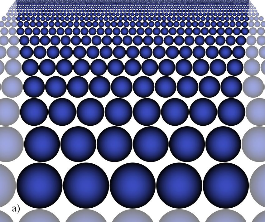
Computation 2020, 8, 9                                                                                  2 of 34

situated in the interference volume. Here, the interference of two beams is considered, resulting in a
sinusoidal energy density distribution [8]

                                                            4πx     θ
                                  Φ ( x, y) = 2Φ0       cos     sin     +1 ,                               (1)
                                                             λ      2

where Φ0 is the fluence of each beam and θ is the intersecting angle between the beams. Accordingly,
two-beam interference patterning generates line-like surface structures with a spatial periodicity

                                                          λ
                                             Λ=                   ,                                        (2)
                                                    2 sin (θ /2 )

the minimum achievable periodic distance being half of the used wavelength, i.e., Λ = λ /2 for θ = π.
The fabrication of repetitive microstructures by means of DLIP, using nanosecond pulses of ultraviolet
laser radiation, was demonstrated on ceramics [1], polymers [2–4,7], non-metals [5] and metals [6].
     A thorough understanding of the process is essential to the precise patterning of surfaces. However,
an insight into the physical mechanisms effective during laser processing cannot be gained from
experimental observation, especially owing to the short laser pulse duration and the microscopic scale
of the surface modification. Nevertheless, numerical simulations enable the detailed investigation of the
contemplated physical effects. This approach allows for parameter variations to identify suitable process
conditions with regard to texturing a specific substrate, avoiding an excessive consumption of resources in
experiments. Grid-based numerical techniques, such as the finite volume and the finite element method
(FEM), are usually employed in the simulation of laser material processing [9].
     The mathematical model of the DLIP process originally consisted in the heat diffusion equation
with the pulsed laser interference irradiation incorporated in the heat source term [8] and sink terms
accommodating the latent heat of involved phase changes [10,11]. Using this model, thermal simulations
of DLIP were carried out by the FEM to predict the temporal evolution of the temperature distribution near
the metal surface and to assess the effect of the laser fluence on the extent of molten and vaporised material
regions [10,11]. For aluminium substrates, the significant increase of the absorptivity with temperature
necessitates the consideration of a temperature-dependent reflectivity in the model [12]. A detailed
description of the FEM simulation of DLIP for metal substrates is presented in [13].
     In this work, the thermal modelling outlined so far is expanded for the first time, according to the
best of the present authors’ knowledge, to comprise the molten bath convection during nanosecond
pulsed DLIP of metal surfaces. The additional complexity of this modelling approach is accepted in the
prospect of insight into the role of melt pool convection in surface patterning and a profound explanation
of the structuring mechanism. Furthermore, the thermofluiddynamic simulations are performed using
the mesh-free smoothed particle hydrodynamics (SPH) technique. The application of mesh-free methods,
which permit a deformation or even disintegration of the computational domain, is comparatively novel
in the simulation of laser processes.
     Specifically, the use of SPH in the modelling of laser material interactions is still little explored.
The SPH method was originally developed by Gingold, Lucy and Monaghan [14,15] to address
astrophysical problems. Notwithstanding its continuing importance in theoretical astrophysics, SPH was
subsequently applied to various problems, notably those involving fluid flow, as in turbomachinery [16],
coastal and hydraulic engineering [17]. A detailed account of these advances can be found in systematic
work [18–21]. Concerning the simulation of laser processing, Chen and Beraun first solved the coupled
heat conduction equations governing ultrashort laser pulse action, i.e., of subpico- to picosecond duration,
on metal films by the corrective smoothed particle method [22].
Computation 2020, 8, 9 3 of 34
The interaction of micro- to millisecond laser pulses or continuous laser irradiation with materials
was modelled more frequently. Gross developed an SPH model for the laser cutting of metals [23], which
was extended by Muhammad et al. to simulate the micromachining of coronary stents [24]. Considering
microsecond pulses as well, Abidou et al. simulated the laser drilling of stainless steel [25]. Earlier on,
Tong and Browne used weakly compressible SPH (WCSPH) to model the melt pool flow and heat transfer
during laser spot welding [26], i.e., for millisecond pulses. Comparable laser spot welding simulations
were performed for metallic workpieces in [27,28]. Regarding continuous irradiation, Yan et al. studied
hydrodynamic interactions during laser underwater machining of alumina by SPH [29]. Later on, Hu et al.
simulated conduction mode [27,30] and deep penetration laser welding [30] of aluminium. Russell et al.
developed a comprehensive SPH methodology for laser based additive manufacturing and applied it
to selective laser track melting [28]. Tanaka et al. investigated also heat conduction due to a stationary
or moving laser source using the moving particle semi-implicit method similar to SPH [31]. In addition
to [28], selective laser melting was modelled by WCSPH in [32–34].
On the contrary, SPH was rarely employed to address the effects of nanosecond laser pulses.
The authors of this manuscript previously suggested a thermal model of DLIP for metallic substrates [35].
Cao and Shin predicted the particle motion due to phase explosion during high fluence laser ablation
of metals by SPH [36]. Further, Alshaer et al. used SPH to simulate the thermal ablation of aluminium
at elevated fluences, particularly the ejection of particles by the recoil pressure [37]. However, the melt
pool flow during nanosecond laser irradiation at moderate fluences was not studied to date using SPH.
According to the best of the authors’ knowledge, an incompressible SPH (ISPH) model was not applied to
the laser-induced molten bath flow before, in contrast to weld pool convection [38].
2. Mathematical Model
This section presents a mathematical model of the material behaviour during single pulse DLIP.
The equations governing the considered physical phenomena are stated and subsequently rewritten in
non-dimensional form to reveal the dimensionless numbers characterising the process.
2.1. Governing Equations
Throughout the DLIP process, the energy conservation is of fundamental importance.
Correspondingly, the mixed enthalpy-temperature formulation of the heat transfer equation reads
dh
ρ = κ∆T + q̇000. (3)
dt
The conservation of mass and momentum is particularly significant while the substrate is molten due
to the effect of the laser pulse. The associated continuity and Navier–Stokes equations are given by
∇ · v = 0, (4)
dv
ρ = −∇ p + η∆v + ρg. (5)
dt
As a Lagrangian method is employed, the evolution of particle positions is governed by
dx
= v. (6)
dt
d ∂
The substantial derivative = + v · ∇ is employed on the left hand side of Equations (3), (5)
dt ∂t
and (6).Computation 2020, 8, 9 4 of 34
In Equation (3), the specific enthalpy h consists of sensible and latent amounts
h = hsens + hlat = cp ( T − T0 ) + f m Lf + f v Lv , (7)
where Lf and Lv are the latent heat of fusion and vapourisation, respectively. On the right hand side
of Equation (3), κ is the thermal conductivity, T the temperature and q̇000 denotes the heat source term.
Considering two-beam interference along with a Gaussian temporal shape of the laser pulse and the
Beer–Lambert absorption law, the source term is given by
2 !
000 Φ ( x, y) t − tp
q̇ ( x, y, z, t) = α (1 − R) √ exp − + α (z − zsurf ) , (8)
σ 2π 2σ2
where Φ ( x, y) is the fluence distribution .
according to
Equation (1), α is the absorption coefficient of the
√
substrate, R is its reflectivity and σ = τp 2 2 ln 2 denotes the standard deviation of the laser pulse
with the duration τp (full width at half maximum (FWHM)) at the pulse time tp .
The molten material is conceived as an incompressible fluid, as evident from the mass and momentum
conservation in Equations (4) and (5). Moreover, the Oberbeck–Boussinesq approximation is applied, i.e.,
the density is constant except in the body force term of the momentum Equation (5), where the density
varies as a function of temperature according to
ρ ( T ) = ρ0 [1 − β ( T − Tl )] (9)
with the volumetric thermal expansion coefficient β. Further, the pressure gradient term in Equation (5)
considers the total pressure comprising static and dynamic components, which is represented as
p = pstat + pdyn = ρ0 g (zsurf − z) + patm + pdyn , (10)
where patm is a constant atmospheric reference pressure at the material surface located at zsurf .
Employing the wavenumber k = 2π /λ in Equation (1), inserting Equation (1) in Equation (8), and
taking the result and Equations (9) and (10) into account in Equations (3) and (5), respectively, the governing
equations take the form
2 !
t − tp
dh 2Φ α θ
ρ0 = κ∆T + (1 − R) √0 cos 2kx sin + 1 exp − + α (z − zsurf ) , (11)
dt σ 2π 2 2σ2
∇ · v = 0,
dv
ρ0 = −∇ pdyn + η∆v − β ( T − Tl ) ρ0 g, (12)
dt
dx
= v.
dt
Due to the short time scale of nanosecond laser interference patterning, heat losses due to convection
and radiation are neglected and the heat transfer equation is subject to adiabatic boundary conditions
∂T ∂h
−κ = 0, = 0. (13)
∂n ∂nComputation 2020, 8, 9 5 of 34
In the presence of melt, homogeneous Neumann boundary conditions are applied to the dynamic
pressure and the no-slip condition, i.e., vanishing velocity, is enforced at the bottom of the molten pool
∂pdyn
= 0, v = 0. (14)
∂n
At the free surface, an inhomogeneous Neumann condition, the Marangoni boundary condition, is
employed for the horizontal velocity, cf. [39,40], and a vanishing vertical velocity is prescribed
∂u ∂γ dγ ∂T
η = = , w = 0. (15)
∂z ∂x dT ∂x
2.2. Non-Dimensionalisation
To rewrite the governing equations in dimensionless form, the non-dimensionalisation of the variables
position, time, velocity, pressure, temperature and specific enthalpy is performed employing the scales L,
L2 / a , a / L , ρ0 a2 L2 , Tv − T0 and cp,ref ( Tv − T0 ), respectively. In particular, the characteristic length scale
√
is specified as the diffusion length L = 2 aτp , where the pulse width τp (FWHM) is chosen as the laser
beam dwell time. Applying the aforementioned scales, the resulting dimensionless variables are
r
∗ x t τp 4τp T − T0 h
x = √ , t∗ = , v∗ = 2 ∗
v, pdyn = p , T∗ = , h∗ = . (16)
2 aτp 4τp a ρ0 a dyn Tv − T0 cp,ref ( Tv − T0 )
Using the dimensionless variables in Equation (16), Equations (4), (6), (11) and (12) are obtained in
dimensionless form as
2
∗ ∗ t ∗ − t∗
dh La 2π x p
= ∆T ∗ + (1 − R) √ cos + 1 exp − + α∗ (z∗ − zsurf
∗
) , (17)
dt∗ ∗
σ 2π Λ ∗ 2σ ∗2
∇ · v∗ = 0, (18)
dv∗ ∗ T∗ − Tl∗
= −∇ pdyn + Pr∆v∗ + PrRa ez , (19)
dt∗ 1 − Tl∗
dx∗
= v∗ (20)
dt∗
with the dimensionless standard deviation σ∗ = σ 4τp of the laser pulse, periodicity Λ∗ = Λ / L and
absorption coefficient α∗ = αL in Equation (17). In particular, the dimensionless form of the Marangoni
boundary condition in Equation (15) is given as [40]
∂u∗ Ma ∂T ∗
=− . (21)
∂z ∗ 1 − Tl∗ ∂x ∗
The dimensionless numbers emerging in the dimensionless Equations (17)–(21), complemented by
the Fourier number Fo corresponding to the considered physical time, are the Laser number La
2Φ0 α tend
La = , Fo = , (22)
ρref cp,ref ( Tv − T0 ) 4τpComputation 2020, 8, 9 6 of 34
the Prandtl number Pr, the Rayleigh number Ra and the Marangoni number Ma defined by
√
β ( Tv − Tl ) g aτp
r
ν dγ Tv − Tl τp
Pr = , Ra = 8τp , Ma = − 2 . (23)
a ν dT ρ0 ν a
In addition, the dimensionless specific enthalpy is obtained as
h∗ = T ∗ + f m Phs/l + f v Phl/v , (24)
where the phase change numbers of melting and vapourisation are defined as
Lf Lv
Phs/l = , Phl/v = . (25)
cp,ref ( Tv − T0 ) cp,ref ( Tv − T0 )
Finally, the molten and vaporised mass fractions required for Equation (24) and the relation between
enthalpy and temperature are given by
h∗ ≤ Ts∗
0
∗ ∗
h − Ts
fm = T ∗ − T ∗ +Phs/l Ts∗ < h∗ < Tl∗ + Phs/l , (26)
l s
∗ ∗
1 Tl + Phs/l ≤ h
∗
∗ 0
h ≤ 1 + Phs/l
h −1−Phs/l
fv = Phl/v 0 < h∗ − 1 − Phs/l < Phl/v , (27)
1 1 + Phs/l + Phl/v ≤ h ∗
h ∗ fm = fv = 0
T ∗ + f T ∗ − T ∗ 0 < f < 1, f = 0
m m v
T∗ = s
∗ − Ph
l s
. (28)
h s/l f m = 1, f v = 0
Tv∗ = 1
f m = 1, 0 < f v ≤ 1
3. Smoothed Particle Hydrodynamics
The mesh-free SPH method employed in the present work is described in the following. The exposition
of the method starts with its fundamentals and then explains the important aspects to be considered to set
up a working SPH algorithm. This account comprises the incompressible SPH (ISPH) approach pursued
to solve the fluid flow along with a discussion of numerical stability.
3.1. Fundamentals of the SPH Method
The mathematical identity underlying the SPH method is the representation of a quantity ϕ by its
convolution with the delta distribution δ given as
Z
ϕ x0 δ x − x0 dx0.
ϕ ( x) = (29)
The kernel approximation is performed by replacing the delta distribution inside the integral in
Equation (29) with a kernel function W, resulting in
Z
ϕ x0 W x − x0, lsm dx0,
ϕ ( x) ≈ (30)
ΩxComputation 2020, 8, 9 7 of 34
where Ω x denotes the compact support of W centred at x and defined by the smoothing length lsm .
The integration in Equation (30) is carried out as a summation over discrete particles representing the
computational domain Ω, giving rise to the particle approximation
N mj
∑
ϕ ( x) ≈ ϕ x j W x − x j , lsm . (31)
ρ
j =1 j
The requirements for the kernel function imposed to establish the approximation in Equation (30)
and further desirable properties are [41,42]
lim W x − x0, lsm = δ x − x0
(approximation of δ distribution), (32)
lsm →0
W x − x0, lsm ≥ 0 ∀ x0 ∈ Ω x
(positivity), (33)
W x − x0, lsm = 0 0
∀x ∈
/ Ωx (compact support), (34)
W x − x0, lsm = W x − x0 , lsm
(spherical symmetry), (35)
W x − x0, lsm ≥ W x − x00, lsm 0 00
∀ x−x < x−x (monotonicity), (36)
Z
W x − x0, lsm dx0 = 1
(normalisation), (37)
Ωx
W ∈ C2 (smoothness). (38)
The existence of a continuous second derivative of the kernel function in condition (38) is imposed [43],
and, in particular, is necessary if it is evaluated in second derivative approximations.
In the present work, a quintic B-spline ascribed to Schoenberg [44], introduced in SPH context by
Morris et al. [45], is employed. In the notation used by Speith [46], this kernel function consisting of
piecewise quintic polynomials is given as
5 5
(1 − r/lsm )5 − 6 32 − r/lsm + 15 13 − r/lsm 0 ≤ r/lsm < 31 ,
5
W (r, lsm ) = d
ς (1 − r/lsm )5 − 6 23 − r/lsm 1
3 ≤ r/lsm < 23 , (39)
lsm
(1 − r/lsm )5 2
≤ r/lsm < 1,
3
0 1 ≤ r/lsm ,
where r = | x − x0|, the problem dimension is denoted by d and the normalisation constant results from
Equation (37) as [46]
243/40 d = 1,
ς= 15309/(478π) d = 2, (40)
2187/(40π) d = 3.
Unlike the representation of the physical quantity ϕ itself in Equation (31), the particle approximation
of a derivative term involves the first derivative of the kernel function, as elucidated in Section 3.2. In case
of the quintic spline kernel function presented above in Equation (39), the first derivative is given as
4 4
(1 − r/lsm )4 − 6 23 − r/lsm + 15 13 − r/lsm 0 ≤ r/lsm < 13 ,
∂W (r, lsm ) −5ς (1 − r/lsm )4 − 6 23 − r/lsm
4 1
≤ r/lsm < 23 ,
= d +1 3 (41)
∂r lsm (1 − r/lsm )4 2
≤ r/lsm < 1,
3
1 ≤ r/lsm .
0Computation 2020, 8, 9 8 of 34
3.2. Approximation of Derivatives
An approximation of the gradient of a scalar field ϕ can be obtained by inserting ∇ ϕ in Equation (30)
and performing an integration by parts [19]
Z
∇x0 ϕ x0 W x − x0, lsm dx0
∇ ϕ ( x) ≈
Ω∩Ω x
Z Z
∇x0 ϕ x0 W x − x0, lsm dx0 − ϕ x0 ∇x0 W x − x0, lsm dx0
= (42)
Ω∩Ω x Ω∩Ω x
I Z
ϕ x0 W x − x0, lsm n x0 dΓ + ϕ x0 ∇x W x − x0, lsm dx0.
=
∂Ω∩Ω x Ω∩Ω x
Concerning the right hand side of Equation (42), the first integral is rewritten as a surface integral
according to Gauss’ theorem. In addition, the symmetry of the kernel function in Equation (35) implies
the property ∇x0 W ( x − x0, lsm ) = −∇x W ( x − x0, lsm ) of the kernel gradient, which is applied to the
second integral.
As the surface integral in Equation (42) vanishes if x is far enough from the domain boundary ∂Ω,
the straightforward approximation of the gradient of a scalar quantity ϕ results as
Z
ϕ x0 ∇x W x − x0, lsm dx0.
∇ ϕ ( x) ≈ (43)
Ωx
Consequently, the discrete particle approximation of the gradient of a scalar field ϕ is given as
Nmj x − x j ∂W x − x j , lsm
∇ ϕ ( x) ≈ ∑ ϕ xj . (44)
ρ
j =1 j x − xj ∂ x − xj
It is remarkable that the derivative of a quantity, e.g., the gradient of a scalar field ϕ in Equation (44),
is evaluated using the quantity at the particle positions and the known derivative of the kernel function,
see Equation (41), in the SPH method. However, if the discrete gradient presented in Equation (44) is
applied to a constant field, the resulting value is not equal to zero [19].
Intending to solve a system of partial differential equations using a mesh-free particle method,
the discrete differential operators are evaluated at the position xi of a particle of interest i in the following.
The zeroth order consistency of the gradient approximation can be recovered by employing the symmetric
gradient operator [19,47]
Ni
1 xi − x j ∂W xi − x j , lsm
Gi− ∑ mj
ϕj = ϕ j − ϕi ≈ (∇ ϕ)i , (45)
ρi j =1 xi − x j ∂ xi − x j
where the shorthand notation ϕi = ϕ ( xi ) is used. On the contrary, it is not recommended to approximate
the pressure gradient in the momentum Equation (5) by the symmetric gradient operator in Equation (45),
as Gi− does not fulfil the action–reaction principle [47,48], i.e., Newton’s third law. Linear momentum
conservation can be ensured using the antisymmetric gradient operator [42,48]
!
Ni
ϕi ϕj xi − x j ∂W xi − x j , lsm
Gi+ ∑ mj
ϕ j = ρi 2
+ 2 ≈ (∇ ϕ)i , (46)
j =1 ρi ρj xi − x j ∂ xi − x j
which satisfies the action–reaction principle.Computation 2020, 8, 9 9 of 34
In view of the accuracy of the projection-based incompressible SPH approach to be presented in
Section 3.4, it is essential that the discrete gradient and divergence operators be skew-adjoint [19,47].
For this reason, the velocity divergence arising in the incompressible SPH scheme is approximated by the
symmetric divergence operator [48]
Ni
1 vj − vi · xi − x j ∂W xi − x j , lsm
Di− ∑ mj
vj = ≈ (∇ · v)i , (47)
ρi j =1 xi − x j ∂ xi − x j
where it can be shown that the discrete operators Gi+ and Di− are skew-adjoint [19].
Moreover, a second-order differential operator, the Laplacian, is required to solve the governing
equations, e.g., for the approximation of the heat conduction term in the heat transfer Equation (3) and the
viscous diffusion term in the momentum Equation (5). If a procedure analogous to the one in Equation (42)
is followed, the resulting expression involves the second derivative of the kernel function [19,46,47].
Therefore, the approximation is very sensitive to particle disorder [48] and plagued by an undetermined
sign of the summands [19,49] as the kernel function exhibits a point of inflexion. On the other hand, a
discrete Laplacian could be constructed by composing a gradient and a divergence operator [19,50], i.e.,
∆i ≈ Di− Gj+ . This exact operator comprises a double summation, which makes it impracticable due to the
high computational effort [19,47].
Nevertheless, an approximate Laplacian can be obtained, as first suggested by Morris et al. [45],
by combining a finite difference expression for the gradient with an SPH divergence operator [47].
The resulting second-order differential operator employs only the first derivative of the kernel function.
This discrete Laplacian originates in the modelling of heat conduction [51,52] and viscous diffusion [45].
Considering the approximation of a general diffusion term, the Laplacian is given by [45,52]
Ni
mj ϕi − ϕ j ∂W xi − x j , lsm
=∑
Li Γϕ,j , ϕ j Γϕ,i + Γϕ,j ≈ ∇ · Γϕ ∇ ϕ i
, (48)
ρ
j =1 j x i − x j ∂ x i − x j
where Γϕ denotes the diffusion coefficient related to the quantity ϕ. The Laplacian Li in Equation (48)
represents a simplified form for a spherically symmetric kernel function. Instead of a scalar ϕ,
the approximate Laplacian can also be applied to a vectorial quantity and the resulting vector is denoted
by Li in this case.
3.3. Boundary Conditions
The treatment of boundary conditions in SPH received little attention from its inception in theoretical
astrophysics, where boundaries do not play a crucial role [53]. Nevertheless, the application of boundary
conditions in an SPH algorithm is a nontrivial task. Particles close to the boundary exhibit an incomplete
kernel support due to the truncation by the boundary, the particle deficiency problem [54].
Different approaches were proposed to remedy the incompleteness of the kernel support near the
boundaries, including three classical boundary treatment techniques. The first is the generation of mirror
particles by direct reflexion of near-wall particles across the boundary, as proposed by Libersky and
Petschek [55]. On the other hand, Monaghan [56] introduced boundary particles, which are located at
the edges of the computational domain and exert repulsive forces on approaching particles. In addition,
Randles and Libersky [54] completed the kernel support of near-wall particles by fixed dummy particles
situated beyond the boundaries.
Furthermore, Kulasegaram et al. [57] devised a profound treatment for wall boundaries using a
variational formulation of the SPH equations of motion. In this approach, a correction factor, i.e., a functionComputation 2020, 8, 9 10 of 34
characterising the completeness of the kernel support, for particles near a wall is introduced and, on its
basis, boundary contact forces are evaluated [57]. Considering the distance of a particle from the nearest
boundary segment, the correction factor and its derivative are determined using a spline approximation of
the original kernel integral [19,57]. Different methods were also developed to account for the case of an
intersection of boundary segments [57].
In the present work, boundary conditions to the energy Equation (3) are imposed using fixed dummy
particles located beyond the boundaries. Moreover, a combination of edge particles situated right on the
boundary and dummy particles is employed to apply the boundary conditions required for the solution
of molten pool convection using the incompressible SPH method presented in the following Section 3.4,
as suggested by different authors [58,59].
3.4. ISPH Approach
The traditional approach of treating incompressible fluid motion using SPH consists of the assumption
of a slight compressibility of the fluid and the numerical solution of the compressible conservation
equations. In addition, this weakly compressible SPH (WCSPH) method comprises an equation of state to
close the system of the compressible continuity and Navier–Stokes equations. However, this procedure
gives rise to considerable noise in the pressure field, since small fluctuations in the density field result in
large pressure fluctuations due to the stiffness of the equation of state [59]. Remedies suggested for this
disadvantage of WCSPH include a particle initialisation algorithm [60] and the introduction of diffusive
corrections [61,62] in combination with a particle shifting approach [63].
More recently than WCSPH, the projection method for the numerical solution of the incompressible
Navier–Stokes equations developed independently by Chorin [64] and Temam [65] was introduced in
SPH context by Cummins and Rudman [50]. The projection method employs the Helmholtz–Hodge
decomposition theorem which states that any vector field w on a smoothly bounded domain Ω can be
uniquely decomposed in the form
w = u + ∇ p, (49)
where u is a solenoidal vector field and parallel to the boundary ∂Ω, and ∇ p is an irrotational vector
field [66].
The SPH approach relying on the projection method for solving the equations governing
incompressible fluid flow belongs to the incompressible SPH (ISPH) methods. Meanwhile, several
ISPH algorithms based on the projection method were proposed using different formulations of
the incompressibility constraint, i.e., imposing either a divergence-free velocity field [50] or density
invariance [58] or combining both criteria [67]. Other than the projection-based approach, an ISPH method
using Lagrange multipliers acting as non-thermodynamic pressures to enforce constant particle volume
was presented in [68].
It was recognised that the sole requirement of zero velocity divergence in a projection-based ISPH
algorithm leads to substantial particle density variations [67], due to the stretching and compression
of particle positions [69]. This particle clustering phenomenon arises due to the ordered motion of the
particles along the streamlines [19,69]. By enforcing density invariance in the projection-based ISPH
algorithm, the problem can be avoided [67], but this method exhibits a reduced numerical accuracy [69].
Combining both zero velocity divergence and density invariance requirements in an ISPH approach, Hu
and Adams could remedy the excessive particle density variations [67].
The latter method being associated with an increased computational effort; Xu et al. proposed an
alternative [69]. This approach combines the projection-based ISPH method enforcing a divergence-free
velocity field with a slight shift of the particle positions across the streamlines [69]. As this ISPH algorithm
is expected to produce acceptable results with reasonable computational effort, it is employed in theComputation 2020, 8, 9 11 of 34
present work. For the numerical solution of the system of governing Equations (4), (6), (11) and (12) in
the time step tn+1 = tn + ∆t, the steps of the algorithm are given below. (The gradient of a vector field in
h iT
Equation (57) is a second-order tensor equal to the Jacobian, i.e., ∇vin+1 = ∇v1,i
n +1
· · · ∇vnd,i+1 .)
x = xn + vn ∆t position advection (50)
n n n
v = v + (ν∆v + β ( T − Tl ) gez ) ∆t velocity prediction (51)
ρ
n +1
∆pdyn = 0∇·v solution of pressure Poisson equation (PPE) (52)
∆t
n +1 ∆t n +1
v = v − ∇ pdyn velocity correction (53)
ρ0
∆t
x n +1 = x n + v n + v n +1 position update (54)
2
000,n+1 ∆t
n +1 n n +1
h = h + κ∆T + q̇ enthalpy update (55)
ρ0
xein+1 = xin+1 + CαRi position shift (56)
vein+1 = vin+1 + ∇vin+1 xein+1 − xin+1 velocity adjustment (57)
T
hin+1 = hin+1 + ∇hin+1
e xein+1 − xin+1 enthalpy adjustment (58)
3.5. Time Step Criteria
The time step size has to satisfy several constraints in order to ensure the numerical stability of the
SPH algorithm. In short, the time step can be determined according to
s s
lsm lsm l2 l2 3
ρlsm
∆t = min 0.25 , 0.25 min , 0.125 min sm , 0.125 min sm , 0.25 , (59)
vmax i | fi | i νi i ai 2πγ
the Courant–Friedrichs–Lewy, maximum particle acceleration, viscous and thermal diffusion, and surface
tension conditions on the time step being given within brackets.
3.6. Neighbour Search
To identify the interacting pairs of neighbouring particles, the cell index method [70] is employed.
This approach was described by Hockney and Eastwood [71] with regard to the evaluation of short-range
forces in particle methods and first used in the SPH method by Monaghan and Gingold [72]. The principal
idea is to subdivide the domain into square cells with a side length equal to or slightly larger than the
interaction radius [70,71]. Each particle is assigned to a cell on the basis of its position. The cells are
represented by an array of linked lists maintained to keep track of the particles residing in each cell [70–72].
Therefore, the search for all neighbours of a given particle reduces to the examination of the particles in the
same cell and in the eight adjacent cells (in 2D) [70,71]. The number of tests required for determining all
interacting particle pairs is further halved in the present case of symmetric interactions. The computational
effort may be further decreased using an optimal, larger cell size [73] or combining the cell linked lists
with a Verlet list, which introduces additional memory requirements [74].
4. Numerical Solution of Governing Equations
The intention of the present work is to perform numerical simulations of heat transfer and fluid flow
during single pulse DLIP using SPH. A 2D section of the substrate in the x − z plane comprising theComputation 2020, 8, 9 12 of 34
interaction zone due to one period of the interference pattern is considered for this purpose, see Figure 1.
This area is discretised using particles as illustrated in Section 4.1. Thereafter, the concrete numerical
scheme employed to solve the dimensionless governing Equations (17)–(20) is presented.
The basic strategy to solve the energy Equation (17) in the computational domain throughout the
simulation duration is shown in Section 4.2. Shortly after the onset of the nanosecond laser pulse,
a thin layer of material adjacent to the surface starts to melt in the vicinity of the interference maximum.
In the subdomain representing the molten pool, the solution of the energy equation is a part of a more
comprehensive approach to solve the complete set of Equations (17)–(20), which is clarified in Section 4.3.
Figure 1. Two-beam interference scheme and computational domain.
4.1. Discretisation
As indicated above, the present research considers a rectangular computational domain in the x − z
plane, which is discretised using particles. The length of the domain is given by the period Λ of the
interference pattern in Equation (2), whereas its height amounts to several diffusion lengths L, as defined
in Section 2.2. To maintain a reasonable computational effort, the employed particle distribution exhibits a
local refinement towards the surface in line with the strategy the authors used before in [35]. In particular,
the interaction zone, where the substrate is expected to melt due to the action of the laser pulse, is
discretised by equidistant fine particles. Despite the associated high computational effort, this idea is
followed to allow for equal size particles in the subdomain representing the molten pool.
In detail, the discretisation is performed starting from the bottom of the computational domain, where
a row of coarse particles of 1 µm diameter is employed. The discretisation is continued using a successive
reduction of the particle size towards the surface, the diameter of the particles in the rows situated
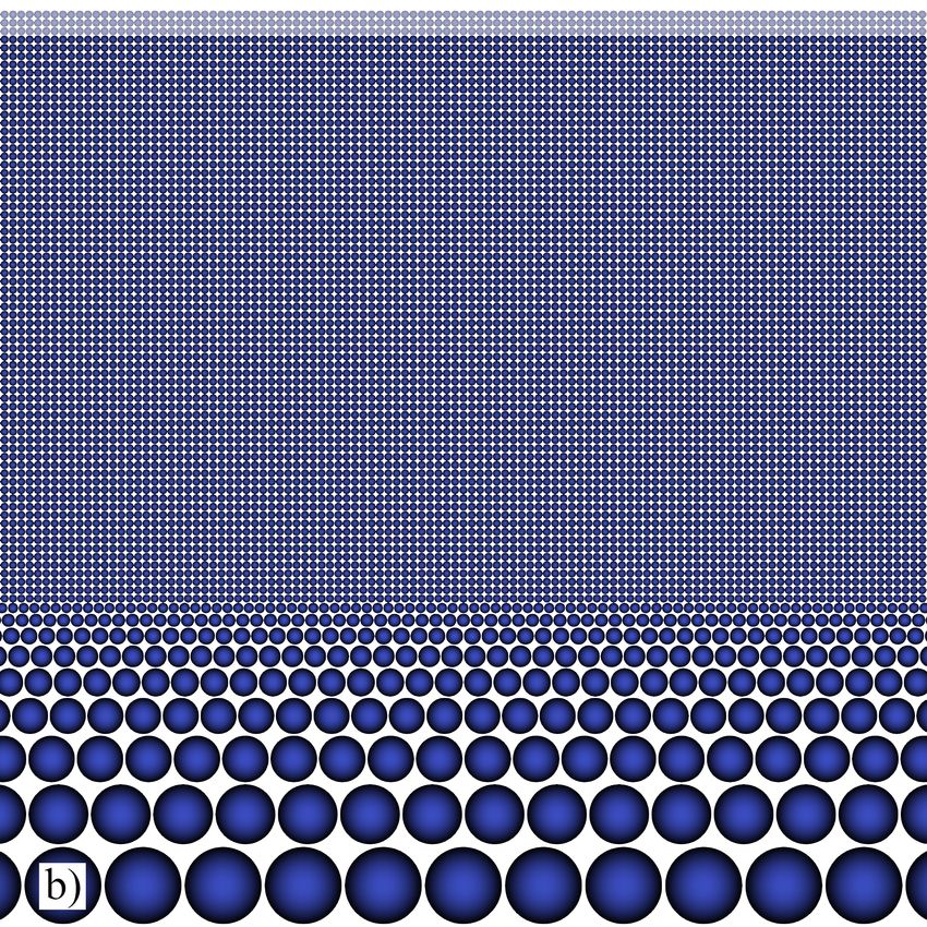
above being given by a geometric sequence with a common ratio, or quotient, of q = 7/9. A graphical
representation of the discretisation is provided in Figure 2, where Figure 2a shows the coarser part referred
to so far. As mentioned in the foregoing paragraph, the refinement does not go beyond a minimum
particle size, and numerous rows of particles of this size are arranged on a Cartesian lattice to discretise the
interaction zone adjacent to the surface, see Figure 2b. The uniform and initially equidistant distribution
of fine particles is employed to avoid potential detrimental effects of different particle sizes during the
numerical solution of molten pool convection. As a trade-off between an appropriate resolution of the
absorption length and a manageable computational effort, the minimum particle diameter is specified as
(7/9)22 µm ≈ 3.97 nm.
In addition, the discretisation is extended by three rows and columns of dummy particles situated
beyond the horizontal and vertical domain boundaries, respectively. Consequently, the kernel function
support of the adjacent interior particles is completed by the dummy particles, with the respective particleComputation 2020, 8, 9 13 of 34
diameter being defined by the one of the nearest interior particle. This provision of dummy particles is
prescribed by the employed smoothing length. The latter is related to the (dimensionless) kernel support
radius rW , which coincides with the number of segments of the radial coordinate in the definition of the
spline kernel function in Equation (39).
Figure 2. Discretisation of computational domain by particles, details of (dummy particles less opaque)
(a) 5 µm × 4.5 µm, showing coarser particles starting from the bottom, and adjacent dummy particles.
(b) 440 nm × 440 nm, fine equidistant initial distribution near the surface and coarser particles below.
As stated by Morris, the number of interacting particles should be augmented for a kernel function
with larger compact support [75]. For the commonly employed cubic spline kernel function, the kernel
support radius is rW = 2 and a typical smoothing length amounts to lsm∗ = 2.4∆x ∗ . As the quintic spline
kernel function exhibits a larger compact support with rW = 3, an extended smoothing length
∗
lsm = 3.75∆x ∗ (60)
is used here, where ∆x ∗ is the initial separation of particles on a Cartesian grid. The smoothing length
specified in Equation (60) corresponds to a neighbourhood of 45 interacting particles in an equidistant
rectangular arrangement with particle spacing ∆x ∗ in d = 2 dimensions.
Note that for interactions between particles of different size, the smoothing length is averaged as
explained in the following. Consider two interacting particles i and j separated by k ∈ N \{0} refinements
given by a geometric sequence with common ratio q < 1, and assume without loss of generality that the
diameter di∗ of particle i is larger than the diameter d∗j = di∗ qk of particle j. The vertical distance between
these two particles can be written as
di∗ k −1 d∗ 1 − qk
z∗j − zi∗ = k∆z∗ji,av = (1 + q ) ∑ q l = i (1 + q ) , (61)
2 l =0
2 1−q
i.e., the vertical separation between these particles is the k-fold average vertical particle distance
di∗ 1 − qk d∗j 1 − q−k
∆z∗ji,av = (1 + q ) = 1 + q −1 . (62)
2k 1−q 2k 1 − q −1
From Equation (60), it is evident that the strength of interaction between particles i and j is
non-vanishing only for k ≤ 3. In particular, the average vertical particle spacing in Equation (62) reducesComputation 2020, 8, 9 14 of 34
to the arithmetic mean of the particle diameters in the case k = 1. The above consideration leads to the
averaged smoothing length used for the interaction between particles i and j
∗ l∗ k −1
lsm,i 1 − qk
∗
lsm,ij = (1 + q ) = sm,i (1 + q) ∑ ql = lsm,ji
∗
, (63)
2k 1−q 2k l =0
∗
where the smoothing length lsm,i for particle i is given by Equation (60) with the particle separation being
equal to the particle diameter, i.e., (∆x ∗ )i = di∗ .
4.2. Thermal model
The energy Equation (17) is solved using the methodology presented earlier by the authors and their
co-authors [35]. In particular, the energy Equation (17) in mixed enthalpy–temperature formulation is
implicitly integrated in time. Consequently, the discretisation of the dimensionless energy Equation (17) in
time for an interior or top edge particle i is written as
hi∗,n+1 − hi∗,n
∗,n+1
= L ∗
1, T + Q̇i∗,n+1 , (64)
∆t∗ i j
where the approximate Laplacian from Equation (48) and the power of the laser heat source per unit mass
Q̇i∗,n+1 are employed in dimensionless form.
In the discrete Laplacian Li∗ (1, Tj∗,n+1 ), the temperature Ti∗,n+1 inside the summation is rewritten as
a function of the specific enthalpy hi∗,n+1 according to Equation (24). Subsequently, Equation (64) can be
rearranged to result in an expression for the specific enthalpy at the new time step [35]
!
∗ ∗,n+1 + f n+1 Ph + f n+1 Ph ∗,n+1 ∗
Ni m j Tj l/v ∂W rij ,lsm,ij
hi∗,n Q̇i∗,n+1
s/l
+ ∆t∗ − 2 ∑ j =1 ρ ∗ m,i v,i
j rij∗,n+1 ∂rij∗,n+1
hi∗,n+1 = . (65)
Ni m j
∗ ∂W rij∗,n+1 ,lsm,ij
∗
∗ 1
1 − 2∆t ∑ j=1 ρ∗ ∗,n+1
j rij ∂rij∗,n+1
Replacing also Tj∗,n+1 in Equation (65) with the equivalent terms from Equation (24), a linear system
of equations is obtained for the enthalpy field at the new time step, which is constituted by the individual
equations for all interior and top edge particles i given as [35]
∂W rij∗,n+1 , lsm,ij Ni m∗ h∗,n+1 ∂W r ∗,n+1 , l ∗
∗
Ni m∗j 1 j j ij sm,ij
1 − 2∆t∗ ∑ h∗,n+1 + 2∆t∗ ∑
∗ ∗,n+1 ∗,n+1 i ρ∗ ∗,n+1
ρ
j=1 j ijr ∂r ij j=1 j rij ∂rij∗,n+1
Ni m∗ f n+1 − f n+1 Phs/l + f n+1 − f n+1 Phl/v ∂W r ∗,n+1 , l ∗
j m,i m,j v,i v,j ij sm,ij
+ 2∆t∗ ∑ ∗ ∗,n+1 ∗,n+1
(66)
j =1 j
ρ r ij ∂r ij
∗ ,n + 1 ∗ 2
2πxi∗,n+1 (t − tp )
( " # )
∗,n ∗ La − +α∗ zi∗,n+1 −zsurf
∗
= hi + ∆t (1 − R) √ cos +1 e 2σ ∗ 2
.
σ∗ 2π Λ∗
Concerning the iterative solution of this linear system of equations, a few aspects of interest are given
in the following. To begin with, the third term on the left hand side of Equation (66) is considered not
to contribute to the system matrix, i.e., the molten and vaporised mass fractions are not conceived as a
function of the unknown enthalpy in the present iteration. Instead, this term is calculated based on the
determination of the molten and vaporised mass fractions from the previous enthalpy iterate.Computation 2020, 8, 9 15 of 34
The formulation in Equation (66) gives rise to a linear system of equations characterised in the
following. The system matrix is symmetric, given particles of equal volume (or equal mass in a uniform
density approach), its main diagonal elements are positive and the matrix is strictly diagonally dominant.
These three properties imply that the matrix is positive definite [76]. The conjugate gradient (CG) method
introduced by Hestenes and Stiefel [77] is commonly used to iteratively solve a linear system with a
symmetric and positive definite matrix.
In the present work, a preconditioned variant of the CG algorithm [78] in conjunction with a Jacobi
preconditioner is employed for the iterative solution of the linear system arising from the discretised
dimensionless heat transfer Equation (64). However, only a single CG step is performed, then the quantities
in Equations (26)–(28) are updated according to the new enthalpy iterate and this iterative procedure
is restarted.
4.3. Thermofluiddynamic Model
As indicated in the introductory paragraph of this section, the subsection at hand provides a detailed
account of the ISPH scheme employed to solve the system of dimensionless Equations (17)–(20) in a manner
analogous to the algorithm given in Equations (50)–(58) for the numerical treatment of Equations (4), (6),
(11) and (12). Due to the intricacy of this approach, the subsection is further subdivided for the sake of
clarity. The numerical details of the individual steps, notably the respective discrete differential operators
employed, of the ISPH algorithm are presented in Section 4.3.1. Aspects to be considered for the numerical
solution of the pressure Poisson equation (PPE), which plays a pivotal role in the projection-based ISPH
method, are covered in Section 4.3.2.
4.3.1. Discrete ISPH Scheme
While the substrate is locally molten as a result of the thermalisation of the interference irradiation
provided by the laser pulse, the melt flow is calculated using the ISPH algorithm explained below.
The particle positions and velocities are evolved for the completely fluid particles inside the molten pool,
whereas the dynamic pressure values are also determined for the surrounding edge particles. In accordance
with the sole solution of the energy Equation (17) presented in Section 4.2, the transition from the old
time step t∗,n to the new time step t∗,n+1 = t∗,n + ∆t∗ is considered for the numerical treatment of
Equations (17)–(20) shown here.
At first, the fluid particles are advected to intermediate positions based on the old velocity
xi∗ = xi∗,n + vi∗,n ∆t∗ . (67)
Considering the acceleration due to viscous and body forces, an intermediate velocity field
T ∗,n − Tl∗
!
vi∗ = vi∗,n + PrLi∗ 1, vj∗,n + PrRa i ez ∆t∗ (68)
1 − Tl∗
is predicted, which is not divergence-free. Subsequently, the PPE for enforcing zero velocity divergence
∗,n+1
1
Li∗ 1, pdyn,j = ∗ Di− ∗ v∗j (69)
∆t
is solved at the fluid particles inside and the edge particles surrounding the molten pool. The intermediate
velocity is then corrected using the gradient of the determined dynamic pressure field to obtain a
divergence-free velocity field
vi∗,n+1 = vi∗ − ∆t∗ Gi+ ∗ pdyn,j
∗,n+1
. (70)Computation 2020, 8, 9 16 of 34
After that, the particle positions are updated using both old and new velocity fields
∆t∗
xi∗,n+1 = xi∗,n + vi∗,n + vi∗,n+1 . (71)
2
The specific enthalpy at the new time step is calculated
hi∗,n+1 = hi∗,n + ∆t∗ Li∗ 1, Tj∗,n+1 + Q̇i∗,n+1 (72)
as discussed above in Section 4.2. To avoid a too orderly particle motion along the streamlines, the particle
positions are slightly shifted [69]
2
Ni
ri∗,av 1 Ni xij∗,n+1
xei∗,n+1 = xi∗,n+1 ∗
+ Cα Ri , Ri = ∑ ∗,n+1
nij , ri∗,av = ∑ rij∗,n+1 , nij = , (73)
j =1 rij Ni j =1 rij∗,n+1
with a constant C ∈ [0.01, 0.1], the shifting magnitude α∗ = max j vj∗,n+1 ∆t∗ and the shifting vector
Ri depending on the average particle spacing ri∗,av and the unit vectors nij . A truncated Taylor series
expansion is then employed to adjust the velocity values to the final particle positions (The discrete
h iT
gradient operator in Equation (74) is characterised by Gi− ∗ vj∗,n+1 = Gi− ∗ v∗x,j,n+1 Gi− ∗ v∗z,j,n+1 .)
vei∗,n+1 = vi∗,n+1 + Gi− ∗ vj∗,n+1 xei∗,n+1 − xi∗,n+1 . (74)
In addition, an analogous adjustment is performed for the specific enthalpy values
∗,n+1
T
hei = hi∗,n+1 + Gi− ∗ h∗j ,n+1 xei∗,n+1 − xi∗,n+1 . (75)
Finally, the adjusted specific enthalpy values are considered for the determination of the molten and
vaporised mass fractions and the particle temperatures Ti∗,n+1 according to Equations (26)–(28).
It is observed that the procedure described above uses two different sets of positions for the particle
approximations during each time step. The discrete differential operators employed in the velocity
prediction, solution of the PPE and velocity correction steps in Equations (68)–(70) rely on the advected
particle positions given in Equation (67). On the other hand, the discrete summations in the specific
enthalpy update, position correction, velocity and specific enthalpy adjustment steps in Equations (72)–(75)
are based on the updated particle positions calculated in Equation (71).
In addition, after the specific enthalpy and temperature update in Equation
(72), the temperature
gradient is determined using the symmetric gradient operator Gi− ∗ Tj∗,n+1 , the horizontal component
being required for the Marangoni boundary condition given by Equation (21) in the next time step.
Furthermore, the ISPH scheme exposed above is subject to restrictions on the dimensionless time step
size. Rewriting Equation (59) in dimensionless form, the conditions to be respected are given as
s r !
l∗ ∗
lsm ∗2
lsm Oh ∗3
lsm
∆t∗ = min 0.25 ∗sm , 0.25 min , 0.125 min ∗2
, 0.125 min lsm , 0.25 , (76)
vmax i f i∗ i Pr i Pr 2π
p
where the Ohnesorge number Oh = ν γL/ρ emerges in the dimensionless surface tension condition.Computation 2020, 8, 9 17 of 34
4.3.2. Solution of PPE
Applying the dimensionless form of the discrete Laplacian and symmetric divergence operator in
Equations (47) and (48), respectively, the zero velocity divergence PPE (69) to be solved is written out as
∗,n+1 ∗,n+1
Ni m∗j pdyn,i − pdyn,j ∂W xi∗ − x∗j , lsm
∗ ∗ ∗ ∗ ∗ ∗ ∗ ∗ ∗
1 Ni m j v j − vi · xi − x j ∂W xi − x j , lsm
2∑ = ∗ ∑ ∗ . (77)
j =1
ρ∗j xi∗ − x∗j ∂ xi∗ − x∗j ∆t j=1 ρ j xi∗ − x∗j ∂ xi∗ − x∗j
The presence of Equation (77), which all fluid particles inside and edge particles bounding the molten
∗,n+1
pool are to satisfy, constitutes a linear system of equations Apdyn = b for the dynamic pressure values.
It should be evident from the explanations given below that the concept of a system matrix A,
although it is not assembled in the numerical code, is meaningful for the solution of the PPE. The dynamic
pressure field to be determined by solving Equation (77) is subject to a homogeneous Neumann boundary
condition, the dimensionless form of the first condition in Equation (14), at the molten pool edges, as
mentioned in Section 2.1. For this type of boundary condition, the technique adopted in this work requires
that the dynamic pressure values at the edge particles are assigned to the respective dummy particles
situated beyond the molten pool edges in the outward normal direction.
The idea is to write the linear system consisting of an equation of the type given in Equation (77) for
∗,n+1 ∗,n+1
each fluid and edge particle i in the form Apdyn = b with a square matrix A, where pdyn is the solution
vector comprising the dynamic pressures of all fluid and edge particles i. Contemplating on the left hand
side of Equation (77) for fluid and edge particles, the structure of the system matrix can be understood
from the following observations. To begin with, as the derivative of the kernel function vanishes at the
origin, the self-interaction of a fluid or edge particle i is neglected.
The notation {iD } is introduced for the set of dummy particles associated with an edge particle i.
In particular, the interactions of an edge particle i with the dummy particles j ∈ {iD } are disregarded
as the dynamic pressure values cancel out. Apart from the interaction with a (different) edge particle j,
each contribution due to the interaction of a fluid or edge particle i with any dummy particle j0 ∈ { jD } by
∗,n+1
means of the value pdyn,j is allocated to the associated edge particle j with equal dynamic pressure. These
considerations lead to the non-zero entries of the matrix A listed in Table 1. In detail, the off-diagonal
elements aij in the second row of Table 1 are valid for both fluid and edge particles i.
Table 1. Non-zero elements in matrix A of linear equation system corresponding to the pressure Poisson
equation (PPE).
Role of Particle
Particle
Fluid Particle Edge Particle
Ni m∗
j 1
∂W rij∗ , lsm
∗ Ni m∗j 1 ∂W rij∗ , lsm
∗
i aii = 2 ∑ ∗ ∗ aii = 2 ∑
ρ r
j=1 j ij
∂rij∗ ρ∗ r ∗
j=1,j6=i j ij
∂rij∗
j 6 =i ∈ { iD }
j/
m∗j 1 ∂W rij∗ , lsm
∗
m∗j 1 ∂W rij∗ , lsm
∗
m∗j0 1 ∂W rij∗ 0 , lsm
∗
j aij = −2 ∗ ∗ ∗ aij = −2 ∗ ∗ ∗ −2 ∑
ρ j rij ∂rij ρ j rij ∂rij ρ∗ r ∗
j0∈{ jD } j0 ij0
∂rij∗ 0
The following properties of the system matrix A can be inferred from its elements presented in Table 1
and further reflexions. In general, the matrix is comparatively sparse since the number of interactions Ni
of neighbouring particles with particle i is much less than the total number of particles representing the
molten pool and its edges. Nevertheless, the situation that each fluid particle can in principle interactComputation 2020, 8, 9 18 of 34
with any other fluid or edge particle throughout the simulation leads to the fact that the matrix is not
banded. It is evident from Table 1 that the main diagonal entries aii of the matrix A are negative, whereas
its off-diagonal elements aij are positive.
The matrix A is weakly diagonally dominant, as ∀i : | aii | = ∑ j6=i aij . More precisely, the sum of
the elements in each row of A is zero. Therefore, the vector x0 = (1, 1, . . . , 1)T is in the kernel of A.
Consequently, the matrix A is not of full rank, i.e., A is singular, according to the rank-nullity theorem.
This problematic feature of A arises for confined flows in the absence of a Dirichlet boundary condition on
the pressure [47,79].
Now consider a fluid particle i situated sufficiently close to an edge so that there is at
least one
dummy particle j0 beyond edge particle j interacting with particle i, i.e., ∃ j0 ∈ { jD } : W rij∗ 0 , lsm
∗ > 0, then
m∗j 1 ∂W rij∗ ,lsm
∗ m∗j0 ∂W rij∗ 0 ,lsm
∗
aij = −2 ρ ∗ r ∗ ∂rij∗
− 2 ∑ j0∈{ jD } ρ∗ r1∗ ∂rij∗ 0
. On the contrary, there is no additional interaction
j ij j0 ij0
allocated to the one with
fluid particle i in the row giving rise to Equation (77) for edge particle j, i.e.,
∗ ∗
m∗ 1 ∂W r ji ,lsm
a ji = −2 ρ∗i ∗ ∂r ∗ji
. Consequently, as aij 6= a ji , the matrix A is non-symmetric.
i r ji
As the system matrix A is not regular as mentioned above, it should be regularised to solve the linear
system of equations. This is performed through a slight reinforcement of the diagonal entries and by
subtracting from the right hand side of the equation system the mean of its entries [47].
In this work, the linear system with a resulting non-symmetric and regular system matrix is solved
iteratively using the BiCGStab algorithm [80]. However, a numerical instability of BiCGStab denoted as
pivot breakdown [81] is often encountered during the solution of the PPE. For this reason, a stabilisation of
the algorithm is implemented, which detects a pivot near-breakdown situation and consequently restarts
the BiCGStab iteration.
5. Simulation Results
In the following, the model presented above is applied to investigate DLIP of metallic substrates
using a single nanosecond pulse. For the sake of clarity, the present section is divided into two
subsections. First, the parameters of the DLIP process are indicated in Section 5.1 along with the material
properties considered for both stainless steel and aluminium substrates as well as the actual values of the
dimensionless numbers. Subsequently, the details of the numerical investigation and the results of DLIP
simulations by means of (I)SPH are presented in Section 5.2.
5.1. Model Parameters
As already indicated above, the interference of two coherent laser beams giving rise to a sinusoidal
intensity distribution is studied in this work. The considered parameters of the DLIP process, particularly
with regard to the laser heat source, are given in Table 2. Note that the periodicity Λ is given as a function
of the laser wavelength λ and the angle of intersection θ between the interfering beams according to
Equation (2). Due to the specification of the thermal diffusion length as the characteristic length scale,
the Fourier number defined in Equation (22) and given in Table 2 depends only on the pulse duration and
the considered physical time, irrespective of the substrate.You can also read