Income, Liquidity, and the Consumption Response to the 2020 Economic Stimulus Payments
←
→
Page content transcription
If your browser does not render page correctly, please read the page content below
Income, Liquidity, and the Consumption Response to the 2020
                Economic Stimulus Payments*

                 Scott R. Baker† R.A. Farrokhnia‡ Steffen Meyer§
                       Michaela Pagel¶ Constantine Yannelis||
                                             January 11, 2021

                                                    Abstract
           The 2020 CARES Act directed large cash payments to households. We analyze house-
       holds’ spending responses using high-frequency transaction data from a Fintech non-profit,
       exploring heterogeneity by income levels, recent income declines, and liquidity as well as
       linked survey responses about economic expectations. Households respond rapidly to the re-
       ceipt of stimulus payments, with spending increasing by $0.25-$0.40 per dollar of stimulus
       during the first weeks. Households with lower incomes, greater income drops, and lower lev-
       els of liquidity display stronger responses highlighting the importance of targeting. Liquidity
       plays the most important role, with no significant spending response for households with large
       checking account balances. Households that expect employment losses and benefit cuts dis-
       play weaker responses to the stimulus. Relative to the effects of previous economic stimulus
       programs in 2001 and 2008, we see faster effects, smaller increases in durables spending, larger
       increases in spending on food, and substantial increases in payments like rents, mortgages, and
       credit cards reflecting a short-term debt overhang. We formally show that these differences can
       make direct payments less effective in stimulating aggregate consumption.

       JEL Classification: D14, E21, G51
       Keywords: Household Finance, CARES, Consumption, COVID-19, Stimulus, MPC, Transaction Linked

       with Survey Data

   * The   authors wish to thank Sylvain Catherine, Arpit Gupta, Jonathan Parker, and Joe Vavra for helpful discus-
sion and comments as well as seminar participants at the MoFiR Banking Workshop, CEPR New Consumption Data
Conference, Virtual AFFECT seminar, Toulouse School of Economics, Columbia Graduate School of Business, Uni-
versity of Chicago Booth School of Business, and the Federal Reserve Bank of Philadelphia. Constantine Yannelis is
grateful to the Fama Miller Center for generous financial support. R.A. Farrokhnia is grateful to Advanced Projects
and Applied Research in Fintech at Columbia Business School for support. We would like to thank Suwen Ge, Spy-
ros Kypraios, Rebecca Liu, and Sharada Sridhar for excellent research assistance. We are grateful to SaverLife for
providing data access and conducting our user survey.
    †
       Northwestern University, Kellogg, NBER; s-baker@kellogg.northwestern.edu
    ‡
       Columbia Business School, Columbia Engineering School; farrokhnia@gsb.columbia.edu
    §
       University of Southern Denmark (SDU) and Danish Finance Institute (DFI); stme@sam.sdu.dk
    ¶
       Columbia Business School, NBER, and CEPR; mpagel@columbia.edu
    ||
       University of Chicago Booth School of Business, NBER; constantine.yannelis@chicagobooth.edu

                                                        1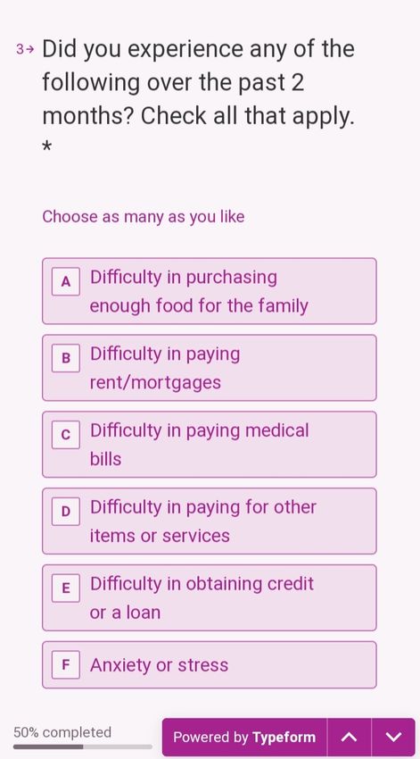
1    Introduction
In three recent instances, the US government made direct cash payments to households in response
to economic downturns. These payments are generally meant to alleviate the effects of a recession
and stimulate the economy through a multiplier effect, i.e., by increasing households’ consumption
which then translates in to more production and employment. The effectiveness of these payments
relies on households’ marginal propensities to consume, or MPCs, out of these stimulus payments
which, in turn, may depend on household’s expectations (Barro, 1989).
    In this paper, we estimate households’ MPC in response to the 2020 CARES Act stimulus pay-
ments using data from a non-profit Fintech firm, SaverLife. We explore how these MPCs vary with
household financial characteristics, such as income, income declines, and cash on hand. We also
describe how household MPCs vary across categories of consumption and how these categorical
responses differ from those seen in previous recessions. Furthermore, this paper links transaction
data to user survey data in order to study how expectations impact household responses to stimulus
payments. Understanding these MPCs is key to targeting policies to households where effects will
be largest, as well as distinguishing between different models of household consumption behavior.
    MPCs are important to both policy and economic theory as they determine fiscal multipliers
in a wide class of models. More specifically, heterogeneity in MPCs impacts which households
are most responsive to stimulus payments. In turn, targeting can have large impacts on the effec-
tiveness of stimulus payments on consumption and the aggregate economy. This paper shows that
liquidity is a key determinant of MPC heterogeneity during the 2020 contraction, with highly liq-
uid households showing no response to stimulus payments. Even among households with higher
levels of income, low levels of liquidity are associated with high MPCs.
    We explore responses to stimulus payments and individual heterogeneity in MPCs by using
high frequency transaction data from SaverLife, a non-profit financial technology firm. Similar to
many other Fintech firms, idividuals can link their accounts to the service to track their finances.
We have access to de-identified bank account transactions and balances data from August 2016
to August 2020 for these users. The fact that we observe inflows and outflows from individual
accounts as well as balances in this dataset allows us to explore heterogeneity in levels of income,
changes in income, and liquidity. The sample consists primarily of lower- and middle-income

                                                 2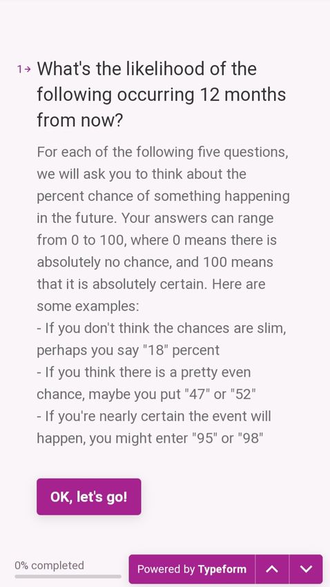
households, and we are able to link the bank account transactions data to survey data about eco-
nomic expectations.
   We use this detailed data to look at the CARES Act stimulus payments distributed in April and
May 2020. The first stimulus payments were made in mid April via direct deposit from the IRS,
and we can observe the user-specific stimulus amounts as well as spending daily before and after
stimulus payments are made. We see sharp and immediate responses to the stimulus payments;
within ten days, users spend over 20 cents of every dollar received in stimulus payments. The
largest increases in spending are on food, non-durables, and payments like rent, mortgages, and
student loans.
   Looking at heterogeneity across financial characteristics, we find that lower income and less
liquidity are associated with larger MPCs while recent drops in income seem to have only small ef-
fects. Individuals with less than $100 in their accounts spend over 40% of their stimulus payments
within the first month, while we observe a statistically insignificant response of only 11 cents for
individuals with more than $4,000 in their accounts.
   These heterogeneity results are important in terms of targeting stimulus policies towards groups
most impacted by them. The theory behind stimulus payments links MPCs directly to the ultimate
fiscal multiplier effect, i.e., the effectiveness of the payments in stimulating aggregate consump-
tion. The results of this study suggest that targeting stimulus payments to households with low
levels of liquidity in a type of recession where large sectors of the economy are shut down will
have the largest effects on MPCs, and hence on fiscal multipliers.
   We further explore how beliefs about personal and aggregate outcomes impact the response to
stimulus payments, utilizing a survey of our users which we can then link to the transaction data.
Theoretical work has long noted that expectations can play an important role in the efficacy of
stimulus (Barro, 1974, 1989; Seater, 1993; Galí, 2019). In particular, households may respond to
debt-financed spending increases by cutting spending today if they anticipate future tax hikes or
other changes in income (Cochrane, 2009), referred to as Ricardian equivalence.
   Discussions about Ricardian equivalence have driven vigorous debates about the efficacy of
fiscal stimulus (Barsky, Mankiw and Zeldes, 1986). In our survey, users are asked about their
expectations regarding unemployment, salary cuts, tax increases, benefit cuts, stock market perfor-
mance, and the duration of the pandemic. We received 1,011 unique responses and find that our

                                                 3
users are relatively pessimistic about the length of the pandemic and their own future income and
employment opportunities.1 While we do not find evidence that anticipated tax increases impact
MPCs, we do find that expectations about employment and government benefit cuts play an im-
portant role in determining MPCs. Households that anticipate unemployment or benefit cuts save
a significantly larger fraction of their stimulus checks.
    We then show in a macroeconomic model with multiple sectors that non-targeted fiscal stim-
ulus payments in environments like the 2020 COVID-19 epidemic may be less effective than the
payments in response to the 2001 and 2008 economic downturns. Reflecting the current situation,
we map out a three sector model in which one sector employing lower wage agents is shut down
while a second low-wage essential sector remains operational alongside a higher-wage sector that
can largely work from home.
    Due to the shut down of one low wage sector, those poorer and higher MPC agents are largely
excluded from benefiting from additional spending induced by stimulus payments, thereby reduc-
ing the fiscal multiplier effect. We also see that agents in the lower wage sectors tend to accumulate
more debt by borrowing from the higher wage sector. Agents end up using the stimulus payments
to repay debt to high wage individuals who have the lowest MPCs out of income. In short, work-
ers will spend their stimulus payment on mortgages and loan repayments as well as non-durable
essentials which implies that the cash flows immediately to agents with lower MPCs. This tends
to make fiscal stimulus less effective overall. This model thus confirms our empirical results.
    There is an extensive literature on households’ responses to tax rebates and previous stim-
ulus payments. Using spending data from the Consumer Expenditure Survey, Johnson, Parker
and Souleles (2006) and Parker, Souleles, Johnson and McClelland (2013) look at the tax rebates
granted in 2001 and the economic stimulus payments in 2008. The authors document positive
effects on spending in both non-durable and durable goods. Broda and Parker (2014) use high-
frequency scanner data and find large positive effects on spending. Besides looking at aggregate
effects, studies have also found heterogeneous effects across agents. Agarwal, Liu and Souleles
    1
      SaverLife conducted our survey from mid-May to the end of July. This survey also elicited self-reported informa-
tion on the receipt and use of the stimulus checks. In terms of the fiscal stimulus use, our survey results line up nicely
with the empirics. 60% of individuals report that they will not use any portion of the check for durables consumption
and 50% of the users are using at least part of the check amount for food spending. A large majority of users also
reported using at least a portion of the stimulus check for payment of current or past due bills. Finally, 15% of users
are reporting to save most of the check amount and 45% report to save none of the check amount.

                                                            4
(2007) work with credit card accounts and find that customers initially saved the tax rebates in
2001, but then increased spending later on. In their setting, customers with low liquidity were
most responsive. Misra and Surico (2014) use a quantile framework to look at the 2001 tax rebates
and the 2008 economic stimulus payments on the distribution of changes in consumption.
       In Section 4.1, we discuss some of the differences between our estimates and the previous lit-
erature that analyze past stimulus programs. The existing studies exploit the differences in timing
of the arrival of the payment to infer causal effects. Our results are generally comparable. How-
ever, the three main differences are: 1) during the 2020 stimulus, households spend much of their
stimulus checks in a shorter period of time, 2) they spend more on food and non-durables than
on durable consumption like furniture, electronics, or cars, and 3) they repay credit cards, rent,
mortgages, and other overdue bills. Additionally, our study is the first to empirically explore, by
linking transaction and survey data, how expectations affect MPCs out of stimulus payments, long
a focus of the theory literature.
       Kaplan and Violante (2014) focus on the 2001 tax rebates and use a structural model to docu-
ment that responsiveness to rebates is driven by liquid wealth. Households with sizable quantities
of illiquid assets but low liquidity are an important driver of the magnitude of the response. To our
knowledge, our study is the first to look at stimulus payments using high-frequency transaction
data, as such data did not exist in 2008.2 The use of transaction data allows us to explore very-
short term responses across categories, minimize measurement error, and explore individual daily
heterogeneity in income declines and available cash on hand.
       In this paper, we focus on a very different type of contraction relative to those faced dur-
ing previous stimulus programs: one stemming from an infectious disease outbreak that caused
widespread business and government shutdowns. In comparison to the 2001 and 2008 economic
downturns, the downturn due to COVID-19 was inflicted on households at a much faster pace,
causing large job losses much more quickly. In addition, the pandemic has the potential to have
large initial effects on income and liquidity, but potentially comparatively less on future income
and wealth.
   2
    A number of papers use transaction-level data to look at spending responses to other income, such as Baker
(2018), Kuchler and Pagel (2020), Olafsson and Pagel (2018), Baker and Yannelis (2017), Baugh, Ben-David, Park
and Parker (2018), and Kueng (2018). Broda and Parker (2014) explore some higher frequency weekly responses
using Nielsen Homescan data.

                                                      5
While previous studies have pointed out that stimulus payments have positive but heteroge-
neous effects on spending, analyzing the 2020 stimulus program will help us learn more about
effects on spending in different economic circumstances. In particular, this crisis was so fast mov-
ing that households had little ability to increase precautionary savings. Additionally, many sectors
of the economy were shut down due to state and local orders, which can impact the effectiveness of
fiscal stimulus, as discussed above. Some policymakers argued that shutdowns make conventional
fiscal stimulus obsolete.3
       Our results are also important for the ongoing discussion of Representative Agent Neo-Keynesian
(RANK) and Heterogeneous Agent Neo-Keynesian (HANK) models. RANK and HANK models
often offer starkly different predictions, and the observed MPC heterogeneity highlights the im-
portance of the HANK framework. In a recent attempt to study pandemics in a HANK framework,
Kaplan, Moll and Violante (2020a) show that for income declines up to 70%, consumption de-
clines by 10%, and GDP per capita by 6% in a lockdown scenario coupled with economic policy
responses. In another recent working paper, Bayer, Born, Luetticke and Müller (2020) calibrate
a HANK model to study the impact of the quarantine shock on the US economy in the case of a
successful suppression of the pandemic. In their model, the stimulus payment help stabilize con-
sumption and results in an output decline of less than 3.5%. Additionally, Hagedorn, Manovskii
and Mitman (2019) study multipliers in a HANK framework, whose size can depend on market
completeness and the targeting of the stimulus.
       This paper also joins a fast-growing literature on the effects of the COVID-19 pandemic on the
economy, and policy responses. Several papers develop macroeconomic frameworks of epidemics,
e.g. Jones, Philippon and Venkateswaran (2020), Barro, Ursua and Weng (2020), Eichenbaum, Re-
belo and Trabandt (2020), and Kaplan, Moll and Violante (2020b). Gormsen and Koijen (2020) use
stock prices and dividend futures to back out growth expectations. Coibion, Gorodnichenko and
Weber (2020) study short-term employment effects and Baker, Bloom, Davis and Terry (2020a)
analyze risk expectations. Granja, Makridis, Yannelis and Zwick (2020) study the targeting and
impact of the Paycheck Protection Program (PPP) on employment. Barrios and Hochberg (2020)
and Allcott, Boxell, Conway, Gentzkow, Thaler and Yang (2020) show that political affiliations im-
   3
     For example, Joshua Rauh the former chair of the President’s Council of Economic advisers noted that: “A
contraction cannot be addressed via conventional fiscal stimulus since no increase in consumer demand will cause
restaurants closed on government orders to re-open.”

                                                       6
pact the social distancing response to the pandemic, and Coven and Gupta (2020) study disparities
in COVID-19 infections and responses.
   Our related paper, Baker, Farrokhnia, Meyer, Pagel and Yannelis (2020b), studies household
consumption during the onset of the pandemic in the United States using a smaller sample drawn
from the same data source. Carvalho, Garcia, Hansen, Ortiz, Rodrigo, Mora and Ruiz (2020),
Andersen, Hansen, Johannesen and Sheridan (2020), Bounie, Camara and Galbraith (2020), Chen,
Qian and Wen (2020) perform similar analyses as the one in this paper using transaction-level data
from the Spain, Denmark, France, and China. Dunn, Hood and Driessen (2020) uses transaction-
level data from the US provided by merchants rather than individual-level data and find similar
results to Baker, Farrokhnia, Meyer, Pagel and Yannelis (2020b). We join this emerging and
rapidly-growing literature by providing early evidence on how households responded to the cri-
sis and on the details of the impacts of federal stimulus policy. The results suggesting that MPCs
are much higher for low liquidity households are important in designing future rounds of stimulus,
as the effects of the epidemic will persist over the next months.
   We also join a literature on how expectations affect household’s economic behavior. Macroe-
conomic models since the 1980s have noted that government budget deficits may in the short-
term affect household’s expectations about future taxes, and implicitly transfers (Barro, 1989). A
newer and growing body of recent work also shows that expectations about individual and aggre-
gate outcomes impact behavior, studying households (Giglio, Maggiori, Stroebel and Utkus, 2019;
Kuchler and Zafar, 2019; Armona, Fuster and Zafar, 2019; D’Acunto, Hoang and Weber, 2020;
Manski, 2004) and firms (Landier and Thesmar, 2020; Landier, Ma and Thesmar, 2017; Bouchaud,
Krueger, Landier and Thesmar, 2019; Gennaioli, Ma and Shleifer, 2016). During the debate about
the efficacy of the 2008 stimulus, the role that expectations would play in the program’s efficacy
and stimulating consumption was discussed at length, however, there is little empirical work ex-
ploring how expectations affect the MPCs out of stimulus payments.
   The remainder of this paper is organized as follows. Section 2 provides background informa-
tion regarding the 2020 stimulus and our empirical strategy. Section 3 describes the main transac-
tion data used in the paper as well as the linked survey data. Section 4 presents the main results and
Section 5 discusses heterogeneity by income, income drops, and liquidity. Section 6 explores how
expectations interact with stimulus payments to affect consumption responses. Section 7 presents

                                                  7
a simple model to explain how fiscal multiplier effects may differ from prior stimulus programs.
Section 8 concludes and suggests directions for future research.
2 Institutional Background and Empirical Strategy
2.1 2020 Household Stimulus
COVID-19, a novel coronavirus, was first identified in Wuhan, China and subsequently spread
worldwide in early 2020. By some estimates, the new virus had a mortality rate which is ten
times higher than the seasonal flu and has at least twice the rate of infection. The first case in the
United States was identified in late January in Washington state and spread within the country in
February. By mid-March, the virus was spreading rapidly, with significant clusters in New York,
San Francisco, and Seattle. Federal, state, and local governments responded to the COVID-19
pandemic in a number of ways: by issuing travel restrictions, shelter-in-place orders, and closures
of many non-essential businesses.
The federal government soon passed legislation aimed at ameliorating economic damage stem-
ming from the spreading virus and shelter-in-place policies. The CARES Act was passed on March
25, 2020 as a response to the economic damage of the new virus. The Act deployed nearly $2 tril-
lion across a range of programs for households and businesses. This study focuses on the portion
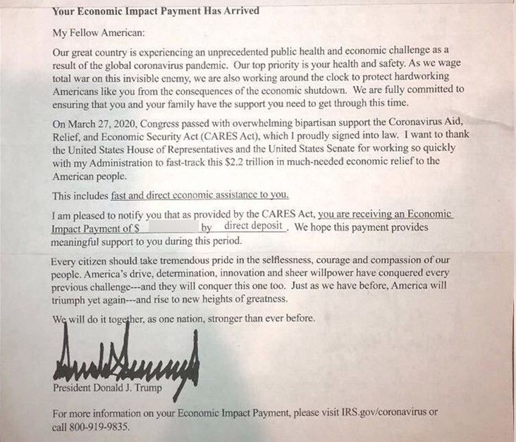
of the Act that directed cash transfers to the vast majority of American households. These one-time
payments consist of $1,200 per adult and an additional $500 per child under the age of 17. For
an overview of amounts by household, see Appendix Figure A.1. These amounts are substantially
larger than the 2001 and 2008 stimulus programs. In 2020, a married couple with two children
would be sent $3,400, a significant amount, particularly for liquidity-constrained households.
Most American households qualified for these payments. All independent adults who have a
social security number, filed their tax returns, and earn below certain income thresholds qualified
for the direct payments. Payments begin phasing out at $75,000 per individual, $112,500 for heads
of households (single parents with children), and $150,000 for married couples. No payments were
made to individuals earning more than $99,000 or married couples earning more than $198,000.4
4
Due to data limitations, in identifying stimulus payments, we are unable to identify these partial payments from
these higher-income households. However, these individuals are a very small fraction of total households, both overall
8
Payments are made by direct deposit whenever available, or by paper check when direct deposit
information was unavailable. Funds are disbursed by the IRS, and the first payments by direct
deposit were made on April 9th. The IRS expected that direct deposits would largely be completed
by April 15th. In practice, the timing varied across banks and financial institutions, with some
making payments available earlier than others, and direct deposits being spread out across more
than one week. Amounts and accounts for direct deposits were determined using 2019 tax returns,
or 2018 tax returns if the former were unavailable.
    For individuals without direct deposit information, paper checks were scheduled to be mailed
starting on April 24th. Approximately 70-80% of taxpayers use direct deposit to receive their tax
refunds, though given changes in banking information or addresses, many individuals were unable
to receive their payments through direct deposit even when they had received prior tax refunds via
direct deposit. In the case of paper checks, the order of payments across households is not random.
The IRS directed to send individuals with the lowest adjusted gross income checks first in late
April, and additional paper checks were sent throughout May. Appendix A provides further details
regarding the timing of payments and the stimulus.

2.2    Empirical Strategy

Our empirical strategy exploits our high-frequency data and the timing of stimulus payments to
capture spending responses. We first show estimates of βk from the following specification:

                                                    23
                                                          βk 1[t = k]it + εit
                                                    X
                                 cit = αi + αt +                                                 (1)
                                                   k=−7

    cit denotes spending by individual i aggregated to the daily level t. αi are individual fixed
effects, while αt are date fixed effects. Individual fixed effects αi absorb time invariant user-
specific factors, such as some individuals having greater average income or wealth. The date fixed
effects αt absorb time-varying shocks that affect all users, such as the overall state of the economy
and economic sentiment. 1[t = k]it is an indicator of the time period k days after receipt of the
stimulus payment for individual i at time t.
    In some specifications, we interact individual fixed effects with day of the week or day of the
and particularly among our sample which is skewed towards lower income households.

                                                      9
month fixed effects to capture individual-level time-varying spending patterns over the week and
month. For example, some individuals may spend more on weekends, or on their paydays. We
run regressions at an individual-day level to examine more precisely the high frequency changes
in behavior brought about by the receipts of the stimulus payments. Standard errors are clustered
at the individual level. The coefficient βk captures the excess spending on a given day before and
after stimulus payments are made. In our graphs, the solid lines show point estimates of βk , while
the dashed lines show 95% confidence intervals.
       We identify daily MPCs using the following specification:

                                                      23
                                                            γk Pi × 1[t = k]it + εit
                                                      X
                                 cit = αi + αt +                                                                      (2)
                                                     k=−7

       where Pi are stimulus payments for individual i. To identify cumulative MPCs since the pay-
ment, we scale indicators of a time period being after a stimulus payment by the amount of the
payment over the number of days since the payment. That is, our estimate of a cumulative MPC ζ
comes from the following specification:

                                                              P ostit × Pi
                                    cit = αi + αt + ζ                            + εit                                (3)
                                                                  Dit

       where Pi is the stimulus payment an individual i is paid, Dit is the total number of days over
which we estimate the MPC, and P ostit is an indicator of the time period t being after individual
i receives a stimulus payment. The coefficient ζ thus captures the aggregate effect of the stimulus
in the time period in question, by scaling the average effect per day by the number of days since
receipt. The resulting coefficients can be interpreted as the fraction of stimulus money spent during
that period: a coefficient of 0.05 corresponds to the user spending 5% of their stimulus check
during their observed post-stimulus period.5
   5
     As an example to illustrate this, imagine that a $1 transfer leads to $1 dollar of additional spending in the day
immediately after receipt. Thus if we estimated the effect over one day, we would scale by 1 and ζ = 1. If we estimate
the effect over 10 days, the average effect each day is 0.1, which would be the coefficient on a regression of P ostit ×Pi
and we scale by 10 so again ζ = 1. If we estimate the effect over 100 days, the average effect per day is 0.01, again
we would scale by 100 and so on.

                                                           10
3 Data
3.1 Transaction Data
In this paper, we utilize de-identified transaction-level data from SaverLife, a non-profit fin-tech
helping working families meet financial goals. As with a number of other personal financial apps,
SaverLife allows users to link their main bank accounts to their service. Users can link their check-
ing, savings, as well as their credit card accounts. The sample is skewed towards lower income
individuals, given that the non-profit fin-tech targets assisting households that have difficulty sav-
ing and meeting budgetary commitments. SaverLife offers users the ability to aggregate financial
data and observe trends and statistics about their own spending.
Figure 1 shows two screenshots of the online interface in the app. The first is a screenshot
of the linked main account while the second is a screenshot of the savings and financial advice
resources that the website provides. This data is described in more detail in Baker, Farrokhnia,
Meyer, Pagel and Yannelis (2020b).
Overall, we have been granted access to de-identified bank account transactions and balances
data from August 2016 to August 2020. We observe 90,844 users in total who live across the
United States. In addition, for a large number of users, we are able to link financial transactions to
self-reported demographic and spatial information such as age, education, ZIP code, family size,
and the number of children they have.
We also observe a category that classifies each transaction. Spending transactions are cate-
gorized into a large number of categories and subcategories. For the purposes of this paper, we
mostly analyze and report spending responses into the following aggregated categories: food,
household goods and personal care, durables like auto-related spending, furniture, and electronics,
non-durables and services, and payments including check spending, loans, mortgages, and rent.
Across all specifications, we exclude transactions that represent transfers between accounts like
transfers to savings or investment accounts.
Looking only at the sample of users who have updated their accounts reliably up until May
2020, we have complete data for 38,379 users to analyze in this paper. We require these users to
have at least 2 transactions in December 2019, at least 5 transactions per month in each month of
2020, and more than 20 transactions adding up to at least $1,000 in total per user. We require 5
11transactions in account usage as a completeness-of-record check for bank-account data following
(Ganong and Noel, 2019).
In Table 1, we report descriptive statistics for users’ spending in a number of selected categories
as well as their incomes at the monthly level. We note that income is relatively low for many
SaverLife users, with an average level of observed income being approximately $36,000 per year.
Note that this observed income is what arrives in a user’s bank account and is therefore post-tax
and post-withholding. In addition, we show the distribution of balances across users’ accounts
during the week before most stimulus checks arrived (the first week of April). Consistent with the
low levels of income, we see that most users maintain a fairly low balance in their linked financial
account, with the median balance being only $98.
We identify stimulus payments using payment amounts stipulated by the CARES Act, identi-
fying all payments at the specific amounts (eg. $1,200, $1,700, $2,400) paid after April 9th in the
categories ’Refund’, ‘Deposit’, ‘Government Income’, and ‘Credit.’ Figure 2 shows the identified
number of payments of this type, relaxing the time restrictions in 2020. While there are a small
number of payments in these categories at the exact stimulus amounts prior to the beginning of
payments, there is a clear massive increase in frequency after April 9th. This suggests that there
are relatively few false positives, and that the observed payments are due to the stimulus program
and not other payments of the same amount.
As of August, approximately 60% of users have received a stimulus payment into their linked
account. The remainder of the sample may have not linked the account that they received the
stimulus check in, be still waiting for a stimulus check, or may be ineligible for one.6 Some banks
and credit unions had issues processing stimulus deposits and these deposits were still pending for
a number of Americans. In addition, users may not have had direct deposit information on file with
the IRS and would then need to wait for a check to be mailed. Finally, users may be ineligible for
stimulus checks due to their status as a dependent, because they did not file their taxes in previous
years, or because they made more than the eligible income thresholds for receipt. Of those who
6
We note that the completeness-of-record checks we employ following (Ganong and Noel, 2019) are relatively
weak. However, keeping a fraction of inactive users in the sample does not affect our results as we can restrict
our analysis to users for which we observe the stimulus payments obtaining the same results. When we look at the
spending behavior of non-stimulus-check recipients around the time when they likely would have received a check,
we do not see a spending response (see Figure A.5) suggesting that these users did not link either their main tax or
spending accounts.
12receive payments, two-thirds received them by April 15, with 40% of all payments occurring on
April 15. 92% of those who received payments in our sample did so in April.
While most American households were due to receive a stimulus check, the amount varied
according to the number of tax filers and numbers of children. Figure A.1 gives an accounting
of amounts due to a range of household types. While we cannot observe the exact household
composition for each user, we are able to observe a self-reported measure of household size. Our
measure matches up reasonably well with the received stimulus payments.
Appendix A provides further details regarding payments in our sample. Payments line up
closely with self-reported household size. Because of our strategy for picking out stimulus checks,
being within the ‘phase-out’ region of income would mean that we would falsely classify an in-
dividual as having not received a stimulus check, since his or her check would be for a non-even
number. This would likely attenuate our empirical estimates slightly. We conduct a placebo exer-
cise in the appendix, and look at spending around April for households that do not receive a check
(see Figure A.5). We do not see any sharp breaks in spending beyond day of the week effects,
suggesting that the impact of mis-categorization is small.
3.2 Survey Data
SaverLife conducted a survey between mid-May to the end of July to elicit self-reported informa-
tion on the receipt and use of the stimulus checks, expectations about personal financial situations,
and the duration of the pandemic. Participants were sent emails and text messages by SaverLife,
and offered $3 to $10 for participation. If individuals did not respond initially, they were sendt
email and text reminders. Users could take the survey on a computer or mobile device, and they
were allowed to skip questions. The survey was sent to 6,060 individuals, who were longer-term
active users of the platform and identified as being potentially responsive to surveys in the past. We
received 1,011 unique responses, indicating a response rate of around 16.7%. The survey questions
are loosely based off of the Federal Reserve Bank of New York Survey of Consumer Expectations.
The survey focused on the following areas:
• Expectations regarding income, the economy and benefits.
• Expectations regarding the length of the pandemic.
13• Self-reported difficulties in paying bills and anxiety.
• Credit.
• Stimulus check spending.
• Political affiliation.
In the online appendix, we report raw survey responses and questions. Figure B.1 shows the
survey instrument on a smartphone, and lists all questions in the survey and Figures B.2 to B.4
show the raw averages of the survey responses. In Figure B.2, we can see that at the time 70% of
the users replied that they received a stimulus check while 15% of the users were still waiting. This
lines up closely with the 66% of users we identify as receiving checks in the data. Additionally,
our user population was subject to a number of financial hardships and subject to difficulties in
payment bills, rents, and mortgages. 30% of users reported they had difficulty obtaining credit and
70% received new credit primarily through a new credit card. Our users are relatively pessimistic
about the lasting effects of the pandemic.
In Figure B.3, we can see that our empirical results in terms of the fiscal stimulus use line up
with the survey data. 60% of individuals report to not use the check amount for durables consump-
tion and 50% of the users are using part of the check amount for food spending. Additionally, only
15% of users said they will not use the check to pay past bills or will use it for future bills. Finally,
15% of users report saving most of the check amount and 45% report to save none of the check
amount.
In Figure B.4, we can see our survey results for expectations other than the duration of the
crisis. Individuals have mixed expectations about the prospects of future stimulus payments and
taxes as well as the stock market. A substantial fraction of users believes they will have lower
7
salaries in the future or become unemployed.
7
Appendix figure B.5 further shows correlations between survey responses as a validation exercise. Households
more pessimistic about stock market performance are more likely to believe that they will become unemployed or see
salary cuts. Households that anticipate tax increases also anticipate benefit cuts, consistent with beliefs about greater
fiscal pressures. Beliefs about unemployment and salary cuts are also highly correlated.
144 Effects of Stimulus Payments
Looking at the raw levels of spending for users receiving stimulus payments, Figure 3 shows mean
daily spending before and after the receipt of a stimulus payment without any other controls or
comparison group. In this figure, we only show spending data for users who receive a stimulus
check in our sample period. Prior to receiving a check, the typical individual in the sample who
receives a stimulus check is spending around $90 per day.8 Mean daily spending rises to about
$250 for the week days after the receipt of the stimulus payment.
To identify the direct impacts of the stimulus check payments, we effectively compare users
receiving stimulus payments to themselves before and after the event as well as to those that did
not receive one on that day. Figure 4 shows estimates of βk from the equation: cit = αi + αt +
k=−7 βk 1[t = k]it + εit . ‘Time to Payment’ is equal to zero for a user on the day of receiving the
P23
stimulus check. Here, we see that users who receive stimulus checks tend to not behave differently
than those that do not in the days before they receive the checks. Upon receiving the stimulus
check, users dramatically increase spending relative to users who do not receive the checks.
There is a sharp and immediate increase in spending following the receipt of a stimulus deposit;
users show large increases in spending in the first days following the stimulus check receipt and
keep spending significantly more than those who have not received checks for the entirety of the
post-check period that we observe. The relative difference in spending declines during weekends,
mostly driven by the fact that observed levels of spending tend to be depressed during these days
for reasons described above.
In Figure 5, we break down users’ spending responses by categories of spending. We map our
categories to roughly correspond to those reported in the Consumer Expenditure Survey: food,
household goods and personal care, durables like auto-related spending, furniture, and electronics,
non-durables and services, and payments including check spending, loans, mortgages, and rent.
Across all categories, we find statistically significant increases in spending following the re-
ceipt of a stimulus check. These responses are widely distributed across categories, with cumula-
tive spending on food, household, non-durables, and payments each increasing by approximately
8
There are substantial intra-week patterns in spending, with Mondays typically seeing the highest levels of posted
transactions and spending as transactions that occurred during the weekend sometimes process only on the Monday
that follows.
15$75-$150 in the week following receipt of a check. Durables spending sees a significant increase,
but it is much smaller in economic terms with only a $20 relative increase in spending during the
first three days.
Table 2 presents similar information, presenting coefficients from the regression cit = αi +
αt + 23k=−7 βk 1[t = k]it × Pi + εit . That is, we examine the excess spending among users who
P
received stimulus payments on each day following the receipt of their stimulus checks, scaled by
the size of their payment. A value of 0.03 can be interpreted as the user spending, on day t, 3% of
their stimulus check (eg. $36 out of a $1,200 stimulus check) more than a user who did not receive
a check. In our sample, the average stimulus check size was $2,166 (median of $1,700).
Columns 1-3 test how total user spending responds with three different sets of fixed effects.
Column 1 presents results using individual and day of the month fixed effects. Column 2 also
includes individual-by-day-of-month fixed effects, and Column 3 includes individual, calendar
date, and individual-by-day-of-week fixed effects. We find similar effects across all specifications,
with spending among those who received a stimulus check tending to increase substantially in the
first week after stimulus receipt.
Spending on days during this period is economically and statistically significantly higher for
those receiving stimulus checks and there are no days with significant reversals – days with stim-
ulus check recipients having lower spending than those who did not. Overall, for each dollar of
stimulus received, households in our sample spent approximately $0.35 more in the month follow-
ing the stimulus.
The remainder of the columns in Table 2 decompose the effect that we see in overall spend-
ing according to the category of spending. We find significant increases in spending in all of
these categories, with the largest increases coming from non-durables and payments. We find
muted effects of the stimulus payments on durables spending. In previous recessions, spending
on durables (mainly auto-related spending) was a large component of the household response to
stimulus checks. At least in the short-term, we find significantly different results, with durables
spending contributing negligibly to the overall household response. We discuss some of these
differences relative to past stimulus programs in Section 4.1.
Because our sample is not representative of the nation as a whole, we also perform a similar
analysis while re-weighting our sample on several dimensions using Current Population Survey
16(CPS) weights. We show results of this approach in Table 3, we compare our estimates from
our unweighted regressions to those using user weights defined on age, sex, state, and income
bins. Column (4) thus runs our primary MPC calculation using these user weights, finding an
MPC of approximately 0.266 rather than 0.369 in column (3). In general, when weighting our
sample to match the national distribution of households more closely, we see qualitatively similar
results approximately 30% lower in magnitudes when weighting along these dimensions. Given
our sample being younger and having lower incomes and assets than the nation as a whole, it is
unsurprising that down-weighting these types of users produces a somewhat lower MPC.
4.1 Comparison to Previous Economic Stimulus Programs
Johnson, Parker and Souleles (2006) and Parker, Souleles, Johnson and McClelland (2013) exam-
ine the response of households to economic stimulus programs during the previous two recessions
(2001 and 2008). These programs were similar in nature to the stimulus program in 2020 but were
smaller in magnitude ($300-600 rather than $1,200 checks).
In these previous stimulus programs, households also tended to respond strongly to the receipt
of their checks. For instance, in 2008, Parker, Souleles, Johnson and McClelland (2013) estimated
that households spent approximately 12-30% of their stimulus payments on non-durables and ser-
vices and a total of 50-90% of their checks on total additional spending (including durables) in the
six months following receipt. In 2001, approximately 20-40% of stimulus checks were spent on
non-durables and services in the six months following receipt.
In one paper examining the high-frequency responses (Broda and Parker, 2014), the authors are
able to use Nielsen Homescan data to examine weekly spending responses to the 2008 stimulus
payments. They find that a household’s spending on covered goods increased by approximately ten
percent in the week that it received a payment. While these authors were not able to examine the
timing of all types of spending due to data limitations, we demonstrate that households respond
extremely quickly to receiving stimulus checks across multiple categories of spending. Rather
than taking weeks or months to spend appreciable portions of their stimulus checks, we show that
households react extremely rapidly, with household spending increasing by approximately one
third of the stimulus check within the first 10 days.
Another notable difference from the stimulus programs is that we find substantially smaller
17impacts on durables spending and confirm this in our survey of users. Previous research has found
strong responses of durables spending to large tax rebates and stimulus programs, especially on
automobiles (about 90% of the estimated impact on durables spending in the 2008 stimulus pro-
gram was driven by auto spending). In contrast, despite a sizable response in non-durables and
service spending, we see little immediate impact on durables. In part, this discrepancy with past
recessions may be driven by the fact that automobile use and spending is highly depressed, with
many cities and states being under shelter-in-place orders and car use being restricted. Similarly,
as these orders hinder home purchases, professional appliance installment and spending on home
furnishings may be lower as well.
Finally, across both 2001 and 2008, Parker, Souleles, Johnson and McClelland (2013) note that
lower income households tend to respond more, and that households with either larger declines in
net worth or households with lower levels of assets also tend to respond more strongly to stimulus
checks. These results are largely consistent with the patterns we observe in 2020. We find that
households with low levels of income and lower levels of wealth tend to respond much more
strongly. In addition, our measure of available liquidity from actual account balances arguably
suffers from much less measurement error than the measures used in previous research on stimulus
checks, giving additional confidence in our estimates.
5 Income, Liquidity, and Drops in Income
The 2020 CARES Act stimulus payments were sent to taxpayers with minimal regard for current
income, wealth, and employment status. While there was an income threshold above which no
stimulus would be received, this threshold was fairly high relative to average individual income
and most Americans were eligible for payments. During debates about the size and scope of the
stimulus, a common question was whether Americans with higher incomes, unaffected jobs, and
higher levels of wealth needed additional financial support. With data on both the income and bank
balances of SaverLife users, we are able to test whether the consumption and spending responses
differed markedly between users who belonged to these different groups.
In Figures 6-8, we show the cumulative estimated MPCs from regressions of spending on an
indicator of a time period being after a stimulus payment is received. Each figure contains the
18results of multiple regressions, with users broken down into subsamples according to a number
of financial characteristics that we can observe. That is, the graphs represent the sum of daily
coefficients seen in a regression as in Table 2, by group. In these figures, we divide the samples of
users by their level of income, the drop in income we observed over the course of 2020, and their
levels of liquidity prior to the receipt of stimulus payments.
Figure 6 splits users by their average income in January and February 2020 (prior to the major
impacts of the pandemic). We see clear evidence that users with lower levels of income tended to
respond much more strongly to the receipt of a stimulus payment than those with higher levels of
income. Users who had earned under $1,000 per month saw an MPC about twice as large as users
who earned $5,000 a month or more.
We also split our sample of users according to their accounts’ balances at the beginning of
April, before any stimulus payments were made. We separate users into multiple groups according
to account balances, from under $10 to over $4,000. Figure 7 displays dramatic differences across
these groups of users. Users with the highest balances in their bank accounts tend not to have
MPCs on the order of 0.1 while those who had under $100 have MPCs of 0.4 or above.
In Figure 8, we examine whether a similar pattern can be seen among users who have had
declines in income following the COVID outbreak. For each user, we measure the change in
income received in March 2020 relative to how much was received, on average, in January and
February 2020. We split users into those who had a decline in monthly income and those who
saw no decline in income (or had an increase). Here we see a significant difference in MPCs,
but of lower magnitude than the previous splits. Households that saw income declines had an
MPC of just over 0.4 while those with no decline in income registered MPCs of about 0.33. This
smaller difference may be driven by the fact that the federal government had also made generous
unemployment insurance available to nearly all workers, mitigating the potential loss of income
from job loss for many lower income households.
Tables 4 - 6 display some of these results in regression form. In general, we find that users
with lower incomes, larger drops in income, and lower pre-stimulus balances tend to respond
more strongly than other users. Again, across all subsamples of our users based on financial
characteristics, we see that low liquidity tends to be the strongest predictor of a high MPC and
high liquidity tends to be the strongest predictor of low MPCs.
196 Expectations and Stimulus Responses
In this section, we explore how household beliefs impact the response to stimulus payments.
Household beliefs may impact MPCs in a number of ways. First, if households anticipate income
declines in the future, they may save more to smooth consumption. Second, if households be-
lieve that taxes or government benefits may change as a result of current fiscal policy or economic
conditions, they will also change consumption decisions. For example, households anticipating
benefit cuts may increase current savings levels. Finally, beliefs about future macroeconomic con-
ditions may also impact household decision-making. On the one hand, if individuals believe that
macroeconomic conditions will improve, they may believe that their own incomes or benefits may
increase, and increase consumption today. On the other hand, individuals may also expect higher
asset returns and invest more out of current resources.
We surveyed over 1,000 users in our sample and asked them about their beliefs regarding
personal unemployment, income, government benefits and taxes, as well as expectations about
the stock market and the duration of the pandemic. We discuss the survey, which was conducted
via mobile device or email, in more detail in section 3.2. We interact these surveyed beliefs with
stimulus receipt and explore how beliefs impact MPCs.
Figure 9 shows MPCs for subgroups, based on user beliefs regarding personal unemployment,
salary cuts, tax increases, government benefit cuts, stock market increases and the duration of the
pandemic. The figure shows cumulative MPCs estimated from coefficients from regressions of
spending on an indicator of a time period being after a stimulus payment, scaled by the amount
of the payment over the number of days since the payment (ζ from cit = αi + αt + ζ P ostDitit×Pi +
εit ). Each bars show individuals above and below the median of the sample in terms of their
expectations.
The top row shows splits by employment outcomes. The left panel splits the sample by in-
dividual beliefs about whether they will become unemployed over the next year. The right panel
splits the sample by individual beliefs regarding whether they will face a salary cut over the next
year. Individuals who believe that they will be more likely to face unemployment or salary cuts see
slightly smaller MPCs, consistent with higher savings in this group. The effect is much larger for
individuals more likely to believe that they will be unemployed, relative to individuals who believe
20that they will face salary cuts.
The middle panel shows splits by outcomes related to government spending– taxes and benefits,
which relates to the classic theory of Ricardian equivalence. The left panel splits the sample by
individual beliefs about tax increases, while the right panel splits the sample by individual beliefs
about government benefit cuts. We see smaller MPCs for individuals who expect tax increases or
government benefit cuts, but the effect sizes are much larger for government benefit cuts. This may
be consistent with the fact that our sample disproportionately includes lower-income individuals
who pay little in taxes, and receive significant government transfers.
The bottom panel splits the sample by expectations regarding whether the stock market will rise
in the next year and whether the duration of the pandemic will last more than two years. Perhaps
surprisingly, we find much smaller MPCs for individuals who expect the stock market to rise. One
potential mechanism is that individuals who believe that the stock market will rise choose to invest
rather than spend. We see little difference for individuals who think that the crisis will be over
within two years, relative to those who think that it will last longer.
Table 7 quantifies this graphical evidence, interacting expectations with stimulus receipt. More
precisely, the table shows MPC estimates and interactions (ζ and ζ 0 ) from the specification:
P ostit × Pi P ostit × Pi × Beliefi P ostit × Beliefi
cit = αi + αt + ζ + ζ0 +ω + εit (4)
Dit Dit Dit
where as before Pi is the stimulus payment an individual i is paid, and Dit is the total number
of days over which we estimate the MPC and P ostit is an indicator of the time period t being after
individual i receives a stimulus payment. Beliefi is the probability that an individual believes that
an event will occur. The coefficient ζ can be interpreted as the aggregate effect of the stimulus in
the time period in question for individuals who do not believe that the mentioned event will occur.
The sum of the coefficients ζ and ζ 0 can be interpreted as the aggregate effect of the stimulus in
the time period in question for individuals who believe that the mentioned event will occur.
Table 7 indicates that beliefs that individuals will be unemployed, government benefits will
be cut, the pandemic will last longer and stock markets will rise are significantly associated with
smaller MPCs. Beliefs about salary cuts or tax increases do not see a statistically significant
21association with MPCs, but the coefficients are negative and this relationship may reflect a lack
of power or the fact that the individuals in our sample pay little in taxes. Overall, our estimates
indicate that beliefs and expectations about personal and aggregate events play an important role
in shaping household responses to stimulus payments.
7 Modeling the Effectiveness of Fiscal Stimulus Payments
In Figure 10, we note the impact of the stimulus check on financial payments. In particular, we
examine the impact on total financial payments as well as payments on several subsets of payments
such as credit card payments as well as rent and mortgage payments. Rent payments are not always
able to be accurately identified due to the number of users who utilize checks or online transfer
tools like Chase QuickPay, Zelle, or Venmo to pay their rent. Such payments will still be accurately
captured by the ‘Total Financial Payments’ category.
We find that financial payments surge substantially upon receipt of the 2020 stimulus payments.
Marginal spending on total financial payments totals about one third of total MPC out of the stimu-
lus payments. We argue that our empirical findings imply that the fiscal stimulus payments may be
less effective in stimulating aggregate consumption in the 2020 environment relative to previous
downturns.
We now present a simple model that outlines two reasons, consistent with our empirical find-
ings, that the fiscal stimulus in 2020 may be less effective in actually stimulating the economy than
the 2001 or 2008 payments. The basic reason for this lack of effectiveness is that sectors of the
economy employing workers with the lowest levels of liquidity are shut down, leading to lower
fiscal multipliers.
Suppose that we have three types of sectors and workers employed by those sectors. First, we
have a sector that we call groceries and necessities. Here, we refer to large firms that sell groceries
and basic household supplies that are both essential and non-durable (moderate depreciation). For
instance, large supermarkets or stores such as Target, Walmart, and CVS. At the same time, the
grocery and necessity sector is moderately labor intensive. This sector is not shut down in response
to an epidemic.
In turn, we have a second sector, called restaurants and hospitality, that produces non-durable
22consumption which depreciates immediately and is more labor intensive than the first sector. Being
less essential to households, the second sector is shut down in response to the crisis.
Finally, we have a third sector of the economy. This sector is broader, and encompasses
durables production as well as many white-collar services like banking and tech. This sector
can avoid being locked down through employing safety measures in production or by working re-
motely. This sector pays higher wages than in sectors 1 and 2. Consequently, the corporations in
sectors 1 and 2 are owned by the workers in sector 3. We assume that workers in sector 1 and 2
borrow (for example, rent, mortgages, or financial lending) from workers in sector 3.
The effectiveness of fiscal stimulus rests on the idea that stimulus checks induce extra spending
by recipients. For example, workers in sector 3 spend in sector 2 and generate income for workers
in that sector that is then spent again. Thus, if the MPC out of a stimulus payment is 0.8, then out
of a $100 payment, $80 is consumed, generating $80 of income for another worker. That worker
then again consumes $64 which generates income for another worker, and so on. In the classic
Keynesian framework the equation for the fiscal multiplier is given by 1/(1 − M P C). The more
cash arrives with agents that have high MPCs, the higher the fiscal multiplier.
In our framework, there are two reasons why fiscal stimulus is less effective in this environment
relative to the 2001 and 2008 recessions. First, in a lockdown induced by an epidemic, neither
group of workers can spend in sector 2. At the same time, workers in sector 2 are the poorest
and have the highest MPCs. Second, workers in sectors 1 and 2 (who are poorer) use the stimulus
payment to pay down debt held by sector 3 workers. Therefore, the excess spending from the
stimulus flows to workers that have a lower MPC.
More formally, we have a three-period model inspired by Guerrieri, Lorenzoni, Straub and
Werning (2020) and consider an economy with three sectors. All sector s agents’ preferences are
represented by the utility function:
3
X
β t U (cst ) (5)
t=0
where cst is consumption and U (c) = c1−σ /(1 − σ) is a standard power utility function. Each
agent is endowed with n̄st > 0 units of labor which are supplied inelastically but they can only
work in their own sector. Competitive firms in each sector s produce the final good from labor
23You can also read