Long-run Effects of Lottery Wealth on Psychological Well-being Erik Lindqvist, Robert Östling and David Cesarini - IFN Working Paper No. 1220, 2018
←
→
Page content transcription
If your browser does not render page correctly, please read the page content below
IFN Working Paper No. 1220, 2018

Long-run Effects of Lottery Wealth on
Psychological Well-being

Erik Lindqvist, Robert Östling and David Cesarini

                                   Research Institute of Industrial Economics
                                                              P.O. Box 55665
                                             SE-102 15 Stockholm, Sweden
                                                                    info@ifn.se
                                                                     www.ifn.se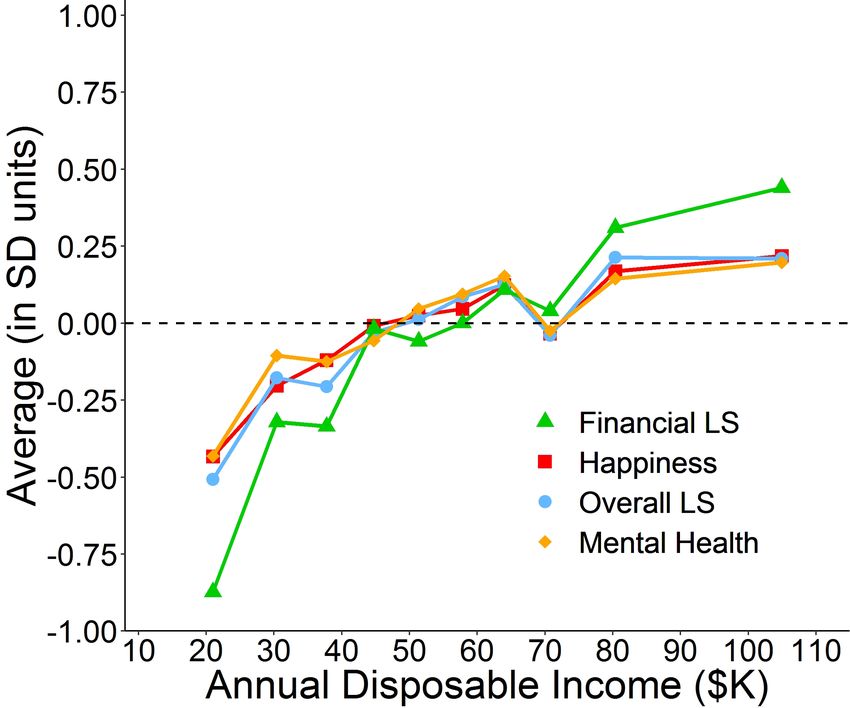
Long-run Effects of Lottery Wealth on Psychological
                                           Well-being

                  Erik Lindqvist, Robert Östling, and David Cesarini*

                                           May 28, 2018

                                               Abstract

          We surveyed a large sample of Swedish lottery players about their psychologi-

      cal well-being and analyzed the data following pre-registered procedures. Relative

      to matched controls, large-prize winners experience sustained increases in overall life

      satisfaction that persist for over a decade and show no evidence of dissipating with

      time. The estimated treatment effects on happiness and mental health are significantly

      smaller, suggesting that wealth has greater long-run effects on evaluative measures of

      well-being than on affective ones. Follow-up analyses of domain-specific aspects of life

      satisfaction clearly implicate financial life satisfaction as an important mediator for the

      long-run increase in overall life satisfaction.

   * Lindqvist: Department of Economics, Stockholm School of Economics, Box 6501, SE-113 83 Stockholm
Sweden, and Research Institute of Industrial Economics (IFN) (e-mail: erik.lindqvist@hhs.se). Östling:
Institute for International Economic Studies, Stockholm University, SE-106 91 Stockholm, Sweden (e-mail:
robert.ostling@iies.su.se). Cesarini: Department of Economics, New York University, 19 W. 4th Street,
6FL, New York 10012, NBER, and IFN (e-mail: david.cesarini@nyu.edu). We thank Agneta Berge, Ed
Kong, Chanwook Lee, Tuan Nguyen and Becky Royer for excellent research assistance. We thank seminar
participants at Columbia, Essex, IFN, HECER, LSE, Michigan, NIPE (Braga), SOFI, Uppsala, Vienna and
Princeton for comments. Daniel Benjamin, Fredrik Bergdahl, Martin Berlin, Samantha Cherney, David
Laibson, Erik Mohlin, Abhijeet Singh and Lise Vesterlund provided especially helpful feedback at various
stages of the project. The study was supported by the Swedish Research Council (B0213903) and the Hedelius
Wallander Foundation (P2011:0032:1). The collection and analysis of the survey data was approved by the
Regional Ethical Review Board in Stockholm on April 7, 2016 (2016/524-31/5).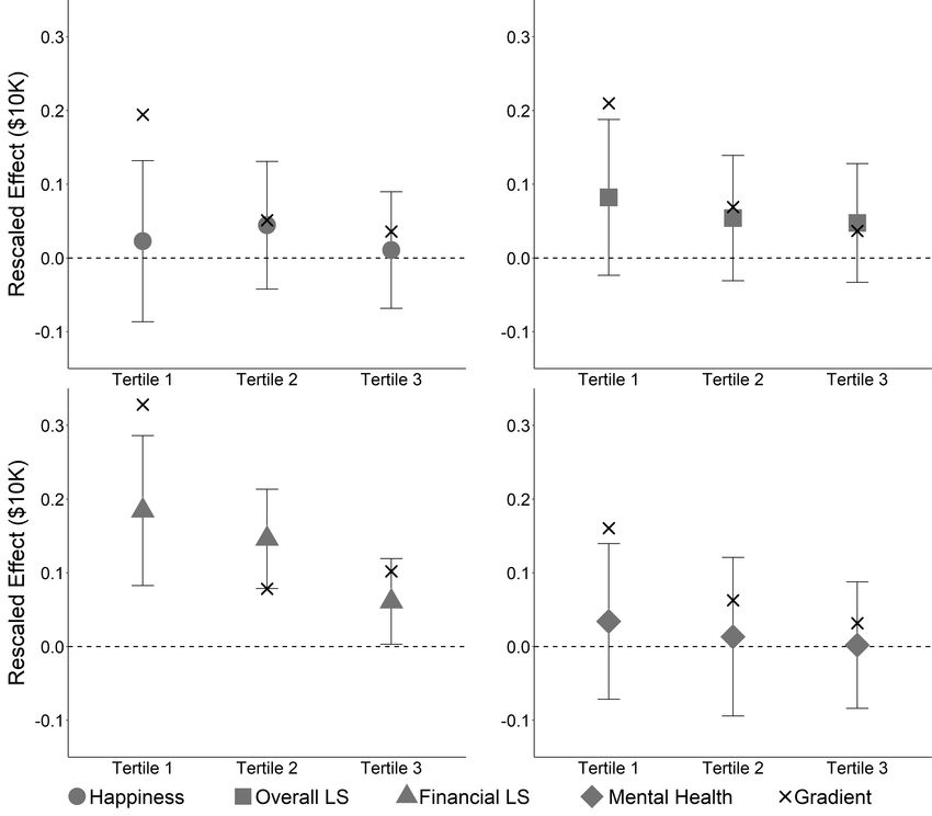
1     Introduction

Observational studies consistently find that happiness, life satisfaction and other facets of
well-being are positively correlated with wealth and income (Diener et al. 1999, Diener &
Biswas-Diener 2002, Biswas-Diener 2008, Sacks, Stevenson & Wolfers 2012, Deaton 2008).
However, the extent to which these associations arise due to causal pathways from wealth to
well-being remains poorly understood (e.g., Frey & Stutzer 2002, Clark, Frijters & Shields
2008, Dolan, Peasgood & White 2008). Considerable uncertainty therefore remains about
the magnitude and persistence of any income or wealth effects on subjective well-being. A
large literature on hedonic adaptation argues that people adjust their aspirations upwards
when their economic conditions improve (e.g., Brickman & Campbell 1971, Frederick &
Lowenstein 1999), implying the long-term effect of positive economic shocks may be small
(Frey & Stutzer 2002, Clark, Frijters & Shields 2008).
    A better understanding of how wealth and income impact long-run well-being is impor-
tant for both societal and individual priorities. At the individual level, people may exaggerate
the importance of financial conditions for well-being (e.g., Kahneman et al. 2006). Estimates
of the effect of wealth may therefore help people who value subjective well-being make more
accurate tradeoffs between pecuniary and non-pecuniary aspects of life (e.g., Layard 2006).
At the societal level, subjective well-being data are increasingly being used in welfare anal-
yses, a topic of ongoing discussion (e.g., Frey & Stutzer 2002, Fleurbaey 2009, Benjamin
et al. 2014). In such settings, estimates of wealth effects may prove valuable, e.g. in cost-
benefit analyses that rely on subjective well-being data to elicit willingness-to-pay for non-
market goods (surveyed in Dolan & Fujiwara 2016).
    To credibly estimate the causal effects of wealth it is necessary to isolate a source of
variation in wealth that is plausibly unrelated to other determinants of well-being. Stud-
ies in developed countries have exploited variation in wealth or income induced by lotteries
(Brickman, Coates & Janoff-Bulman 1978, Lindahl 2005, Gardner & Oswald 2007, Kuhn
et al. 2011, Apouey & Clark 2015), tax rebates (Lachowska 2017), or within-person changes

                                               1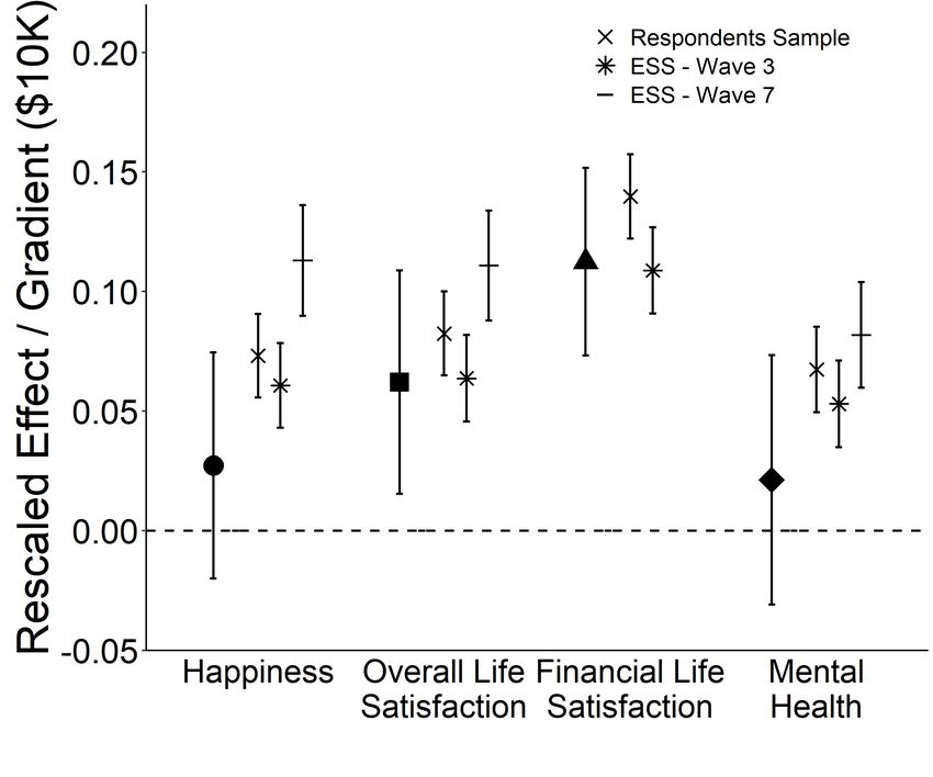
over time (e.g., Frijters, Haisken-DeNew & Shields 2004, Frijters et al. 2006). These stud-
ies overwhelmingly conclude effects are positive, but the effect sizes vary substantially in
magnitude.1 Moreover, with the exception of Lindahl (2005), these studies do not consider
long-term effects.
       In this paper, we study long-run effects of wealth on well-being by leveraging the ran-
domized assignment of lottery prizes in a sample of Swedish lottery players. We surveyed
lottery players about their well-being 5 to 22 years after the lottery event. Our study has
several methodological strengths. First, our data allow us classify players into groups within
which we know the prize amount won is randomly assigned. Our estimates are based entirely
on comparisons of players who are in the same group but were awarded prizes of different
magnitudes. Second, because of the large sample size (3,362 players) and substantial prize
pool ($277 million), our estimates have high precision relative to other work. Third, all main
results are based on pre-registered analyses described in a publicly archived Analysis Plan
(Östling, Lindqvist & Cesarini 2016).
       We find that the long-run effects of wealth vary depending on the exact dimension of
well-being.2 There is clear evidence that wealth improves people’s evaluations of their lives
as a whole. According to our estimate, an after-tax prize of $100,000 improves life satisfac-
tion by 0.037 standard-deviation (SD) units. We find no evidence that the effect varies by
years-since-win, suggesting a limited role for hedonic adaptation over the time horizon we
analyze. Our results suggest improved financial circumstances is the key mechanism behind
the increase in life satisfaction. In contrast, the estimated effects on our measures with a
   1
     Most studies in low- and middle income countries also find positive effects of wealth or income on well-
being. For example, unconditional cash grants have been shown to improve short-run subjective well-being
in Kenya (Haushofer & Shapiro 2016) and Malawi (Baird, de Hoop & Özler 2013), though not in Ecuador
(Paxson & Schady 2010). Relatedly, a study of Chinese twins reports that the positive relationship between
income and happiness persists in within-family analyses (Li et al. 2014). Hariri, Bjørnskov & Justesen (2015)
finds that a decrease in real income induced by a currency devaluation in Botswana had large negative effects
on subjective well-being.
   2
     In the psychometric literature, it is common to make a distinction between affective and evaluative
measures of well-being (Diener et al. 1999, Schimmack 2008). Measures derived from responses to questions
about the frequency of various positive or negative feelings are classified as affective whereas questions that
require respondents to report their evaluation of their life (or some aspect of their life) are often referred to
as cognitive or evaluative.

                                                       2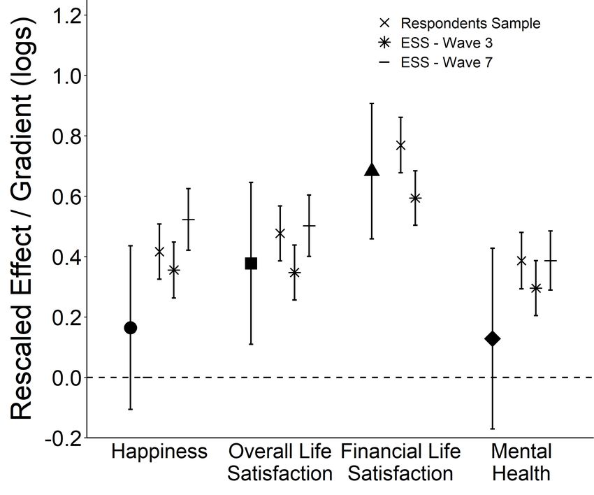
stronger affective component – happiness and an index of mental health – are smaller and
not statistically distinguishable from zero. Despite the strong correlation between happiness
and life satisfaction in our data (0.86), we can statistically reject equal treatment effects of
lottery wealth on these outcomes.
    To help benchmark our results, we rescale our lottery-based estimates and compare them
to gradients with respect to annual income (averaged over multiple years to smooth out
transitory fluctuations). For happiness and mental health, our rescaled estimates are about
one third the magnitude of the corresponding gradients. For life satisfaction, we find that our
rescaled estimate is similar in magnitude to the income gradient. We also compare our main
results to those reported in previous quasi-experimental studies of lottery players’ well-being
and show our study compares favorably both in terms of statistical power and the credibility
of our causal inference.
    Our paper is structured as follows. Section 2 describes our survey of lottery players and
describes the representativeness of our estimation sample. Section 3 describes our identi-
fication strategy and provides evidence in support of our key identifying assumption that
lottery prizes are randomly assigned conditional on factors we observe. Section 4 summarizes
the results from our main analyses and benchmark our estimates against the cross-sectional
gradients and previous lottery studies. Section 5 concludes with a broader discussion of our
findings and their limitations. The Online Appendix contains appendix figures and tables
and additional details about our analyses.

2     Data and Study Design

Our study was conducted in three stages. First, we identified a Survey Population composed
of individuals from a large administrative sample of lottery players. Second, Statistics Swe-
den surveyed these individuals on our behalf. Third, Statistics Sweden supplied us with an
anonymized data set with subjects’ survey responses and administrative variables. For all

                                               3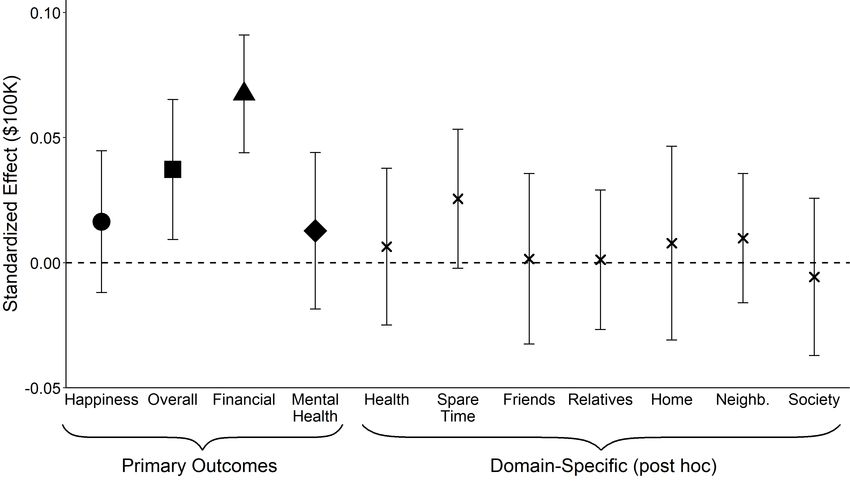
members of the Survey Population, including non-respondents, we have information about a
set of basic demographic characteristics from Swedish registers and lottery-specific variables
needed to implement our empirical strategy.
   The analyses reported in this paper follow the procedures specified in an Analysis Plan
(Östling, Lindqvist & Cesarini 2016) publicly accessible via the URL https://osf.io/
t3qb5/ and archived before the survey data were made available to us. The purpose of
preregistration was to minimize readers’ concerns about data-mining and undisclosed spec-
ification searches and to make transparent the distinction between pre-registered and post
hoc analyses. All aspects of the main analyses were fully specified before the survey data
were delivered to us. Specifically, we pre-specified the criteria for inclusion in the estima-
tion sample; three diagnostic tests for endogenous attrition; our set of primary outcomes;
variable coding (including handling of missing values and outliers); the estimating equation;
heterogeneity and robustness analyses, and how we intended to adjust the p-values for our
primary outcomes for multiple-hypotheses testing.
   In formulating the plan, our goal was not only to reduce the number of investigator de-
grees of freedom in our main analyses, but to eliminate them altogether. We successfully
executed the pre-registered analyses without having to make any additional judgment calls
due to omissions or ambiguities in the Analysis Plan. The Analysis Plan also described
our intention to benchmark our final estimates to household-income gradients and estimates
previously reported in quasi-experimental studies. These comparisons were conducted ac-
cording to the pre-registered procedures. However, we made no attempt to fully specify
every detail of these comparisons before accessing the survey data.

2.1    Survey Population

The Survey Population was drawn from a large administrative sample that has been used in
several previous studies on the impact of wealth on register-based outcomes such as health,
mortality and children’s outcomes (Cesarini et al. 2016), labor supply (Cesarini et al. 2017)

                                              4
and participation in financial markets (Briggs et al. 2015). In determining which members
of the administrative sample to survey, a primary goal was to retain as much as possible of
the lottery-prize variation.
We survey players from three of the four lotteries in the administrative sample: Kombi,
Triss-Monthly and Triss-Lumpsum.3 Kombi is a monthly subscription lottery with approxi-
mately 500,000 subscribers, the proceeds of which are donated to the Swedish Social Demo-
cratic Party. The administrative sample contains information on the number of lottery
tickets and large prizes won for all Kombi participants between 1998 and 2011. Triss is a
highly popular scratch-off lottery run by the Swedish government-owned gaming operator,
Svenska Spel. We have information on two types of Triss prizes which qualify the winner to a
daily TV show where the size of the prize is determined by a new lottery draw. At the show,
Triss-Lumpsum winners (1994 to 2011) win a lump-sum prize between $7,000 and $700,000.
Winners of the Triss-Monthly prize (1997 to 2011) win a monthly income supplement. The
size ($1,400 to $7,000) and duration (10 to 50 years) of the supplement are determined by
separate tickets which are drawn independently. We convert the Triss-Monthly to net-present
value using a discount rate of 2 percent.
To define the Survey Population, we first identified all winners from the Triss lotteries
and all large-prize winners from Kombi (defined as players who won at least 1M SEK). We
then imposed a number of sample restrictions summarized in Table A1. The Analysis Plan
contains a detailed description of, and motivation for, each restriction. By far the most
important restriction is that we only survey individuals aged at most 75 in 2016, the year of
the survey. Applying the full set of sample restrictions left 259 large prizes from Kombi, 3,294
Triss-Lumpsum prizes and 608 Triss-Monthly prizes. We supplied information about these
winners to Statistics Sweden, who dropped prizes won by individuals who were deceased
or lacked an official Swedish address of residence in 2016. In a final step, they added four
3
We elected not to survey participants in the fourth lottery used in our prior studies – the prize-linked
savings accounts (PLS) – because nearly all of the large lottery prizes in this sample were awarded in the 1980s
and 1990s, making it less likely that we would be able to detect treatment effect on an outcome measured
in 2016. An additional consideration was that a substantial fraction of the PLS players are deceased.
5controls for each large-prize winner in Kombi to the Survey Population. The four controls
were randomly selected from the set of non-winning Kombi players whose sex, year of birth
and number of tickets owned exactly matched those of the winner in the month of win.
This leaves our Survey Population of 4,840 observations: 241 Kombi large-prize events and
964 (241Ö4) matched controls, 3,065 Triss-Lumpsum prizes and 570 Triss-Monthly prizes.
Because a small number of individuals appear more than once, these 4,840 observations
correspond to 4,820 unique individuals.4
2.2 Survey Protocol
In early fall of 2016, Statistics Sweden mailed a letter of invitation to all members of the
Survey Population (see Figure A1 for summary of the timeline). The letter was accompanied
by the survey, a return envelope, and a 100 SEK gift certificate. To reduce experimenter
demand effects, the letter made no mention of lotteries.5 Subjects who failed to return
the survey after the first mailing were sent three reminders. Triss-Monthly players who had
failed to return a survey after the third reminder were also contacted by telephone and asked
to return the mail-in survey. (For budgetary reasons, we limited the telephone reminders
to non-respondents from Triss-Monthly). Three weeks after the end of the regular data-
collection via mail, Statistics Sweden tried to reach 501 randomly selected non-respondents
by telephone. Subjects who answered the phone were invited to participate in an abbreviated
phone version of the survey.
4
Individuals may appear in the data more than once because they won the lottery on more than one
occasion, because we draw the controls in Kombi with replacement, or because of overlap between the
lottery samples.
5
The final data set delivered to us contains subjects’ survey responses and some basic socioeconomic
variables from administrative registers. Statistics Sweden required that information about these registers
be available to interested subjects, along with information about the selection of the Survey Population.
To accommodate this requirement, the cover letter referred survey invitees interested in learning more
to a website with information about the registers and details on the selection of the Survey Population.
Unbeknownst to the subjects, each letter’s website URL was unique, and the final data delivered to us
therefore contains information about which subjects accessed the website. Only six subjects did, implying
any resulting biases are likely to be negligible.
62.3 Respondents Sample
Statistics Sweden received mail-in surveys from individuals corresponding to 3,251 of the
4,840 observations of the original Survey Population. Another 111 players (out of 501)
participated in the abbreviated telephone survey, bringing the total response rate to 69%.6
We refer to the survey respondents as our Respondents Sample. Table 1 shows the survey
response rate and the distribution of prizes won for each lottery and our pooled sample.
Here and in all that follows, lottery prizes are net of taxes and measured in units of year-
2011 dollars. Although the majority of prizes are modest, most of our identifying variation
comes from prizes in the range $100,000 – $800,000.7 Even though the Respondents Sample
constitute less than 1% of the pooled lottery sample analyzed in Cesarini et al. (2016), the
oversampling of large-prize winners ensures that about one third of the identifying variation
in lottery wealth in the administrative sample is retained.
Table 2 compares the distribution of pre-lottery baseline characteristics of the individuals
in the Respondents Sample and the Survey Population with a random sample of Swedish
adults. The representative sample has been reweighted to match the sex- and age distribution
in the Respondents Sample. Players are substantially more likely to be born in Sweden (92.4%
versus 83.8%). However, the representative sample was drawn in 2010 and the fraction of
the Swedish population that is foreign-born grew steadily in the lottery years. Therefore, the
observed difference understates the representativeness of players in most lottery years. Play-
ers are similar to the Swedish population in terms of marital status and number of children
residing in their household. They are less likely to have attended college but have higher
labor incomes, on average. In both cases, the differences are modest (25.8% versus 30.1%
and $35,000 versus $32,000, respectively). Overall, the similarity in baseline characteristics is
6
The effective response rate varies between outcomes because not all respondents respond to all questions
in the mail-in survey and because the abbreviated phone survey did not include all questions.
7
One way to quantify the importance of large prizes is to consider the change in treatment variation (the
number of observations times the variance in lottery prizes demeaned at the level of the groups defined in
Section 3) when prizes above some cutoff are dropped. For example, dropping the 415 prizes above $200,000
(column (5) of Table 1) reduces treatment variation by 91%.
7reassuring, though we cannot rule out that players who select into the lottery differ from the
population in unobservables in ways that could impair the generalizability of our findings.
2.4 Primary Outcomes
The Analysis Plan defined four primary outcomes. The first outcome, Happiness, is based on
the respondent’s answer to the question “All things considered, how happy would you say that
you are?” The respondent is asked to select one response alternative among 11 numerically
coded options ranging from 0 (“Extremely unhappy”) to 10 (“Extremely happy”). Our
second outcome, Overall Life Satisfaction (Overall LS, for short), is derived from the answer
to the question “Taking all things together in your life, how satisfied would you say that you
are with your life these days?” The respondent is asked to select an option from an 11-point
scale ranging from 0 (“Extremely dissatisfied”) to 10 (“Extremely satisfied”).
Our third outcome, Mental Health, is constructed from responses to the 12-item version
of the General Health Questionnaire (Golberg & Williams 1988). Originally developed as
a screening instrument for mental health, the GHQ-12 is commonly used to measure an
individual’s level of psychological well-being. Each item requires respondents to indicate, on
a four-point scale, how often during the last two weeks he or she has experienced a specific
positive or negative emotion. The response category chosen on each item is then converted
to an integer between 1 and 4, with higher values indicating greater well-being. The final
variable is defined as the sum of the 12 numerical values, and is hence in the range of 12 to
48, with higher values denoting greater well-being.
Our fourth primary outcome is Financial Life Satisfaction (Financial LS, for short), one
of nine domain-specific aspects of life satisfaction measured in our survey. Each domain
was measured by a single question with a six-point response scale ranging from 1 (“Very
dissatisfied”) to 6 (“Very satisfied”).
Researchers often make a conceptual distinction between evaluative (sometimes referred
to as cognitive) and affective components of subjective well-being (Diener et al. 1999, Schimmack
82008). Happiness is a hybrid of these two dimensions, because our measure is based on a
question with a clear evaluative component (“All things considered...”), yet at the same
time asks about pleasant feelings. By contrast, Overall LS and Financial LS are evaluative:
respondents are required to form an assessment, either of their life as a whole, or of their
overall financial situation. Finally, our measure of Mental Health is affective, as the items
included in the battery all ask about the frequency with which the respondent has recently
experienced a range of pleasant and unpleasant feelings. Despite their differences, Over-
all LS and Happiness are highly correlated both with one another (0.86) and with Mental
Health (0.70 in both cases). Financial LS is modestly positively correlated with each of the
three other primary outcomes, with correlations ranging from 0.39 (Mental Health) to 0.46
(Overall LS ).
3 Analytic Framework
3.1 Estimation and Identification Strategy
Our identification strategy exploits the fact that the lottery prizes in our samples are ran-
domly assigned conditional on player characteristics we observe. We estimate the long-run
causal impact of lottery wealth by ordinary least squares, using the following estimating
equation:
(1) yis = αLi,0 + Zi,−1 γ+Xi β + εi ,
where the time of the lottery event is normalized to t = 0. yis is a measure of well-being
standardized to unit variance for respondent i measured s years after the lottery event.
Because we survey people who participated in lotteries between 1994 and 2011 in 2016, s
varies between 5 and 22. Li,0 is the prize (in $100,000) awarded to individual i at t = 0
and Zi,−1 is a vector of baseline characteristics measured at year-end in the year prior to the
lottery event. Xi is a set of indicator variables for groups of lottery players within which
9the prize money is randomly assigned. We control for the “baseline controls” Zi,−1 solely to
improve statistical precision.
In Kombi, we construct the group identifiers in Xi by assigning each large-prize winner
to the same group as his or her matched controls (occasionally, large prize winners in the
same draw have identical ticket balances, are of the same sex and share a year of birth;
when this happens we assign multiple winners to the same group identifier). In the two Triss
lotteries, two players share a group identifier if and only if they won the same type of prize
(Lumpsum or Monthly) in the same year and under the same prize plan. Because the prize
plan determines the distribution from which prizes of either type are drawn, conditioning on
prize plan guarantees the size of the lottery win is random.
Throughout, we report p-values based on analytical standard errors that have been clus-
tered (Zeger & Liang 1986) at the individual level. In our main analysis of the primary
outcomes, we also report permutation-based p-values constructed by simulating the dis-
tribution of the relevant test statistic under the null hypothesis of zero treatment effects
(Young 2017). In each simulation iteration, we independently permute the prize column in
each group. We next use Equation (1) to generate an estimate of the treatment effect of
wealth. Repeating this process 10,000 times gives us a simulated distribution that we use to
calculate the probability of observing a test statistic as extreme as the one observed under
the null hypothesis. Finally, in our main analyses of the primary outcomes, we also report
p-values that have been adjusted to account for the fact that we examined four primary
outcomes. To calculate these family-wise error rate adjusted p-values, we apply the free
step-down resampling method of Westfall & Young (1993). In the tables, we refer to the
resulting p-values as FWER-adjusted p-values.
In our estimating equation, yis depends linearly on Li,0 even though the true relationship
is likely to be concave. However, from a life-cycle perspective, the concavity is modest as
long as the lottery prize is not very large relative to lifetime income. For example, suppose
well-being is linear in log lifetime income and consider a household with remaining pre-win
10lifetime income of $1.37 million, the approximate median in our sample.8 For a $400,000
prize, the derivative of yis with respect to lifetime income is 1/1.37 for the first dollar won
and 1/(1.37+0.4) for the last dollar, implying a linear specification offers a decent first
approximation to the data.
3.2 Survey Non-Response and Tests of Endogenous Attrition
A potential concern about our identification strategy is that lottery wealth directly influences
survey participation, potentially introducing endogeneity in the Respondents Sample, even
if our identifying assumption holds in the Survey Population. To test for such selection
biases, we conducted three pre-registered diagnostic tests for endogenous selection. All were
conducted and reported exactly as described in the Analysis Plan (pp. 8-13). In test one,
we found no evidence that survey participation is affected by lottery wealth (Table A2). In
test two, we found no evidence of imbalance in baseline covariates measured prior to the
lottery in neither the Survey Population nor the Respondents Sample (Table A3). In test
three, we found that the estimated effects of lottery wealth on net wealth, debt, capital
income and labor income do not change systematically when we restrict attention to the
Respondent Sample by omitting the survey non-respondents from the estimation sample
(Table A4). Overall, the results from these diagnostic tests bolster the credibility of our
causal estimates, to which we now turn.
4 Results
4.1 Primary Outcomes
Figure 1 displays our estimates of the long-run effect of lottery wealth on each of the pri-
mary outcomes (see Table 3 for the underlying data). For all outcomes, we estimate positive
The median annual household disposable income in year t = −1 was $47,000 in our sample. The lifetime
8
income we use in our heApriluristic calculation is simply the product of this income figure and 29, the
median remaining lifespan of lottery players in their year-of-win assuming a lifespan of exactly 80 years.
11effects of lottery wealth. The estimated effects on Overall LS and Financial LS are, respec-
tively, 0.037 SD units and 0.067 SD units per $100,000 won, and remain significant after our
multiple-hypothesis adjustment. For Happiness and Mental Health, the corresponding point
estimates are 0.016 and 0.013, respectively.9 Neither estimate is statistically distinguishable
from zero, but for both outcomes, we can reject treatment effects equal to those found for
Overall LS and Financial LS.10 It is noteworthy that we can rule out equally sized treatment
effects of wealth on Overall LS and Happiness (p < 0.001), despite their very high pairwise
correlation (0.86).
Table A5 reports the results from two pre-specified robustness tests. In the first, we
reweight the sample so that the share of phone-survey respondents in the estimation sample
matches the population share of mail-in survey non-respondents (33%). The reweighted
estimates for the two primary outcomes measured by the telephone survey – Overall LS and
Happiness – are similar to the main results. In the second, we rerun the analyses omitting
players who won prizes above 4M SEK ($580,000). For all outcomes the coefficient estimates
are similar to the baseline results, though with larger standard errors.
To explore potential mechanisms, we conducted post hoc analyses of seven domain-
specific measures of life satisfaction. The results of these analyses are shown in in Figure 1
(see Table A6 for the underlying estimates). For each of the seven outcomes – health, spare
time, friends, relatives, home, neighborhood and society overall – we can rule out treatment
effects as large as those found for Financial LS and, except for a marginally significant ef-
fect on spare time, none of the estimated effects are statistically distinguishable from zero.
Overall, these post hoc analyses suggest that Financial LS mediates much of the observed
9
We note that our estimate of the effect on Mental Health (0.013) is similar to the appropriately rescaled
reduction in consumption of prescribed mental health drugs of 0.023 SD units in our previous work on lottery
winners’ health (Cesarini et al. 2016).
10
In post hoc analyses, we also reran the analyses of Happiness, Overall LS and Financial LS using the
”blow-up and cluster” conditional logit estimator proposed by Mukherjee et al. (2008) which has recently
been shown to work well in a related context (Baetschmann, Staub & Winkelmann 2015). For Happiness and
Overall LS the point estimates are nearly identical, whereas the effect of wealth on Financial LS increases
modestly (from 0.067 to 0.080).
12long-run treatment effect of lottery wealth on Overall LS.11
The claim that the long-run, positive, effect of lottery wealth on Overall LS is mediated by
improved Financial LS may seem hard to reconcile with a common folk wisdom according to
which lottery winners routinely squander their wealth. Yet previous analyses of the Swedish
administrative sample have found little evidence in support of the hypothesis that winners
often consume frivolously following a win. Large-prize winners appear to enjoy sustained
improvement in economic conditions that are robustly detectable for well over a decade after
the windfall (Cesarini et al. 2016). Winners reduce their labor supply and gradually spend
down the windfalls, but the reductions are modest, do not seem to depend on the type of
prize (lump-sum or monthly installments), and spread out quite evenly over the entire time
horizon for which we have post-lottery outcomes (Cesarini et al. 2017). They also invest a
substantial share of the wealth in financial assets, often opting for low-risk bond products
over equities (Briggs et al. 2015).
This evidence is well in line with conclusions from interview-based research on lottery
winners in multiple countries (Kaplan 1987, Furåker & Hedenus 2009, Eckblad & Lippe 1994,
Larsson 2011). For example, one study of American lottery winners concludes matter-of-
factly that “contrary to popular beliefs, winners did not engage in lavish spending sprees”
(Kaplan 1987, p. 168).
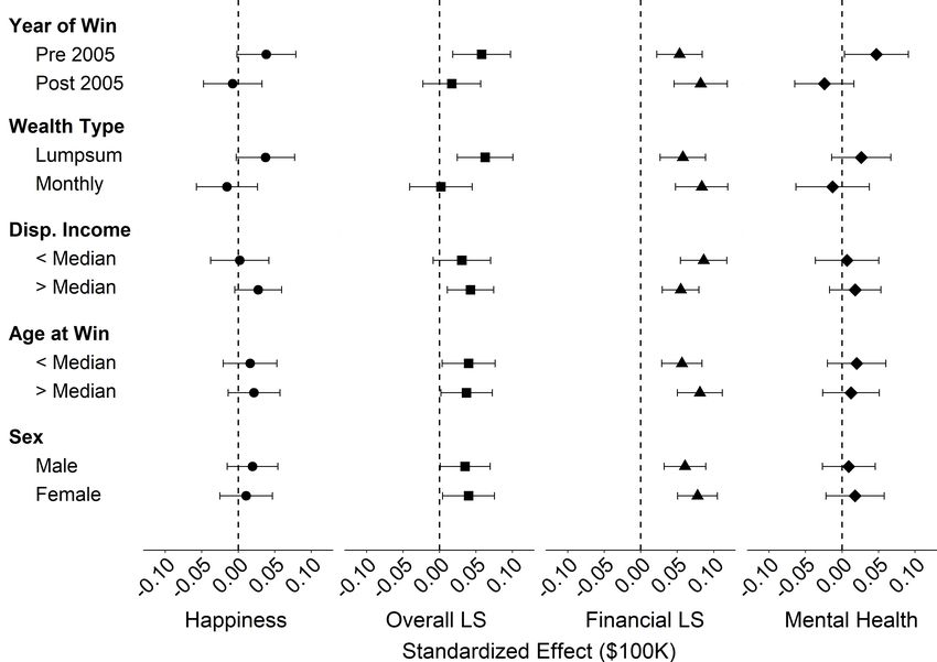
4.2 Heterogeneity
Again following pre-registered procedures, we reran our analyses in subsamples stratified
by sex, age-at-win (below or above median), pre-lottery income (below or above median),
years-since-win (before or after 2005) and type of prize (Triss-Monthly vs Triss-Lumpsum).12
The results are shown in Figure 2 (see Table A7 for underlying data). Overall, the estimated
11
Including Financial LS as an additional control in Equation (1) (similar to a Sobel mediation test)
reduces the estimated effect of lottery wealth on Overall LS by 73%.
12
As explained in our Analysis Plan, we exclude Kombi altogether in the heterogeneity analysis by type
of prize because Triss-Lumpsum and Triss-Monthly winners are drawn from the same underlying population
(people who procure Triss scratch-off lottery tickets). Excluding Kombi makes it less likely that any observed
heterogeneity is due to factors correlated with winning a lumpsum prize.
13treatment effects are similar across subsamples. For example, the long-run effects of lottery
wealth on Financial LS and Overall LS show up quite consistently, with significant treatment
effects (p < 0.05) on Financial LS in all eight subsamples.
We performed 20 tests of homogeneous effects (4 outcomes × 5 dimensions of hetero-
geneity) and we only reject the null hypothesis of equal effects (at nominal p < 0.05) in two
instances: Overall LS by type of prize (Triss-Monthly vs Triss-Lumpsum) and Mental Health
by years-since-win (before or after 2005). This is only one more rejection than expected by
chance under the null hypothesis of homogeneous effects and overall, our analyses therefore
provide no strong evidence of heterogeneous effects. We note that in our analyses by type
of prize, the overall pattern of results is in the opposite direction to what one would expect
if prize money paid as monthly installments helped winners with self-control smooth con-
sumption. Our subsample analyses only yield clear evidence of a positive treatment effects
among players who won lumpsum prizes.13
One notable finding is that the positive effects show little evidence of fading with the
passage of time. Even when we restrict the sample to players surveyed at least 11 years after
the lottery event (“Pre 2005”) the treatment-effect estimates range from 0.038 SD units (p
= 0.062) for Happiness to 0.058 SD units (p = 0.004) for Overall LS. To further explore
how treatment effects vary by years-since-win, we conducted post hoc analyses, the results
of which are summarized in Figure 3 (see Table A8 for underlying estimates). The estimated
treatment effects on Financial LS decay with the passage of time, but for the remaining
three outcomes, the pattern is in the opposite direction. The absence of fade-out suggests
that there is little adaptation to the lottery win over the time window for which we have
data (5-22 years after the lottery event). But this conclusion is subject to the caveat that
year-of-win is not randomly assigned, so it is possible that early and late winners differ along
some dimension that moderates the effect of wealth. Nevertheless, there is little doubt that
13
The comparison between Triss-Lumpsum and Triss-Monthly is potentially confounded by non-linear
effects of wealth. Since Triss-Monthly players win larger prizes, on average, non-linear effects of lottery
wealth could produce heterogeneous effects across the Triss samples even if prizes with identical net present
values have identical effects.
14adaptation to the windfall is incomplete well over a decade after the lottery event.
4.3 Household-Income Gradients
Since lump-sum lottery prizes represent one-time increases in lifetime wealth, there is no
unassailable method for comparing our causal estimates to the cross-sectional income corre-
lations that have been the focus in much of the literature. However, the evidence that many
players choose to spread out the gains fairly evenly and over long time horizons suggests that
players often treat the windfall as a long-run supplement to annual income flows from other
sources (Cesarini et al. 2016, Cesarini et al. 2017, Briggs et al. 2015). Following our Analysis
Plan, we therefore convert each lottery prize to the annual payout it could sustain if it were
annuitized over a 20-year period at an actuarially fair price, and rerun our main analyses
with this alternative scaling. For example, a $100,000 prize corresponds to an increase in
net annual income of $5,996.
We compare our annuity-rescaled treatment effects for each primary outcome to gradients
estimated using a measure of household permanent income (average disposable income over
the period 2004-2014), controlling for sex, a fourth-order polynomial in age and sex-by-
age interactions. Because income is endogenous to the lottery outcome (Cesarini et al.
2017), we estimate the gradients only for individuals in the Respondents Sample who won
prizes below $20K. The average prize won in this sample ($8,491) is small enough that any
endogeneity is likely to be negligibly small. In preliminary analyses, we verified that the cross-
sectional relationship between permanent annual income and our primary outcomes replicate
standard patterns from the literature. Figure A2 shows that in our sample, the cross-
sectional relationship between permanent annual income and each of our primary outcomes
is positive and concave (Deaton 2008, Stevenson & Wolfers 2013). We also compare our
rescaled treatment effects to gradients for Swedish respondents in two waves of the European
Social Survey.14
14
See Section 2 in the Online Appendix for details on the ESS gradients.
15We compare our lottery estimates to the cross-sectional gradients in three different anal-
yses, the first two of which are shown graphically in Figure 4 (see Table A9 and A10 for the
underlying data from all three analyses). The upper panel of Figure 4 shows the rescaled
estimates and gradients when well-being is assumed to be linear in household income. The
rescaled estimates for Happiness and Mental Health are about one third as large as the
gradients, whereas the rescaled estimates for Overall LS and Financial LS are similar in
magnitude to the gradients. For both Happiness and Mental Health, we reject the null
hypothesis that the causal effect is equal to the gradient.
It is common in the literature to assume well-being is linear in log income. To better
compare our results to previous work, we therefore further rescale our lottery-based estimates
to make them comparable to log-income gradients.15 The lower panel of Figure 4 shows
the log-income gradients fall within the normal range previously reported in rich countries
(Stevenson & Wolfers 2013), and that the relationship between gradients and our lottery-
based estimates is similar to the linear case. The causal effect of log income on Overall LS
implied by our estimate (0.377) is thus similar to the log income gradient, while the implied
effect for Happiness is substantially lower (0.165).
Finally, in Figure 5, we repeat the original linear analysis, but in subsamples stratified by
permanent-income tertile. Here, the gradients are estimated using a piece-wise linear spline
regression with two knots, one at each of the cutoff points that define the permanent-income
tertiles. In the bottom income tertile, our treatment-effect estimates are bounded away from
the income gradients (all p < 0.045), as shown in Figure 5. At medium and high incomes,
the gradients are similar in magnitude to the causal estimates.
15
To accommodate the linear-log functional form assumption, we calculated the natural logarithm of the
sum of permanent income (based on pre-lottery income data only) and the annuitized prize. Our final
estimates are from an instrumental variable analysis that uses lottery prizes to instrument for the log of the
sum of permanent income and the annuitized prize. (We also tried alternative methods to accommodate the
functional-form assumption with very similar results.)
164.4 Previous Lottery Studies
We identified five previous quasi-experimental studies of lottery players’ well-being. Table 4
provides summary information about how our study compares to these studies along some
key dimensions: outcome variables analyzed, lottery data used, effect sizes reported and
identification strategy. To facilitate comparisons, the effect-size estimates have been rescaled
for comparability with our main results in Table 3 (effects of $100,000 on an outcome with
unit variance). Section 3 in the Online Appendix provides further details on the calculations
underlying the data in Table 4. Here, we emphasize that cross-study comparisons based
on data in the table are subject to two important interpretational caveats. First, even
though most studies used survey measures similar (in several cases, identical) to ours, only
one (Lindahl 2005) analyzed a long-run measure of lottery players’ well-being. Second, the
rescaled estimates are calculated under the simplifying assumption that the effect is linear
in prize amount.
The first study listed (Brickman, Coates & Janoff-Bulman 1978) famously compared the
happiness of 22 major lottery winners of the Illinois State Lottery to that of 22 controls
domiciled in the same regions as the winners. The study found no statistically significant
differences between winners and controls in terms of happiness (past, present or expected
future). After re-scaling, we obtained a treatment-effect estimate of 0.014 with a standard
error of 0.025. These rescaled estimates are therefore quite similar to what we report for
Happiness, both in magnitude (0.014 vs 0.016) and precision (0.025 vs 0.014). However, the
prizes won by the 22 lottery players are very large compared to lottery winners in subsequent
studies, including ours, with an average prize of $1.18M (range $123K to $2.46M). The
rescaled estimates we report for Brickman, Coates & Janoff-Bulman (1978) are therefore
likely to be the most sensitive to plausible violations of the linearity assumption.
The next two studies listed reported large and positive effects of wealth on mental health,
one using data from Sweden (Lindahl 2005) and the second using British data (Gardner &
Oswald 2007). Apouey & Clark (2015) updated and extended the analysis of Gardner &
17Oswald (2007) in several ways, including controlling for individual fixed effects in the analyses
and adding data from survey waves that have subsequently become available. The follow-
up study reported positive and statistically significant effects on life satisfaction and mental
health measured two years after the lottery (but not on outcomes measured sooner). The next
row shows information from a study of Dutch Postcode Lottery winners (Kuhn et al. 2011),
finding a negative but statistically insignificant effect of lottery wins on happiness. The
four studies that appeared after Brickman, Coates & Janoff-Bulman (1978) had rescaled
estimates with standard errors at least 7 times larger than ours. Therefore, conditional on
finding a statistically significant effect, the effects reported were very large compared to ours.
If the true effect-parameters of these studies are not dramatically different from the effects
we can rule out with high statistical confidence, these studies were under-powered.16
Of course, it may be inappropriate to use our estimates to inform calculations of the likely
power of these other studies. For example, short-run effects of wealth may be substantially
larger than long-run effects. The pattern of results is not easy to reconcile with this theory,
however, since Kuhn et al. (2011) report a negative effect on happiness six months after the
lottery and Apouey & Clark (2015) report larger treatment effects on outcomes measured
two years after the lottery than on outcomes measured in the post-lottery year. This theory
also fails to account for the results in the study that, like us, analyzed a long-run measure of
well-being (Lindahl 2005). A second possibility suggested by the prize data in Table 4 is that
the studies relied to a greater extent on identifying variation generated by small and modestly
sized prizes. When we drop the largest prizes from our data, the estimated treatment effects
increase for two out of four outcomes (Table A5). However, the implied non-linearity for
these two outcomes is not nearly large enough for this factor alone to rationalize the stark
16
To illustrate, suppose the true treatment effect on Mental Health in the previous studies was 0.044 SD
units, the upper limit of the 95% confidence interval of our estimate. Then the statistical power of the
three previous studies reporting statistically significant effects on mental health (Lindahl 2005, Gardner &
Oswald 2007, Apouey & Clark 2015) ranged from 5.02% to 6.55% (at α = 0.05). Conditional on finding a
statistically significant effect, design calculations (Gelman & Carlin 2014) show that studies with such power
will incorrectly sign the effect (“type S error”) between 15% to 45% of the time, and overestimate (absolute
value of) the effect size (“type M error”) by a factor of at least five.
18differences in effect sizes across studies.
The final column of Table 4 summarizes each study’s identification strategy, yet another
potential source of between-study heterogeneity in effect-size estimates. Brickman, Coates
& Janoff-Bulman (1978) compared winners to controls from approximately the same area
as the winners (recruited via phone books). Of the four remaining studies, only one (Kuhn
et al. 2011) compares the outcomes of players from the same lottery, controlling for factors
(e.g. lottery tickets) conditional on which the prizes in the lottery were randomly assigned.
5 Concluding Discussion
Our study leverages the randomized assignment of lottery prizes to generate estimates of
the long-run effects of wealth on four facets of psychological well-being. Our estimates have
strong internal validity and were obtained through pre-registered analyses. Overall, our
study advances understanding of the broader question of why wealth and well-being often
go hand in hand by providing credible and precise estimates of the long-run causal impacts
of large changes in wealth in a sample of Swedish lottery players.
We find that lottery wealth causes sustained increases in Overall LS. Since we did not
survey any players within five years of the lottery, our research design is not suitable for
studying short-run adaptation, but our results do reject the strong hypothesis of complete
adaptation. The effect shows no evidence of fading over the time horizon for which we
have data and is robustly discernible over a decade after the lottery event. Our follow-up
analyses suggest that the most important mechanism explaining the increase in Overall LS
is increased satisfaction with personal finances. A sustained increase in Financial LS is not
easy to reconcile with a common folk wisdom that lottery winners squander their wealth
through wreckless spending. However, consistent with the previous qualitative evidence
(Kaplan 1987, Eckblad & Lippe 1994, Hedenus 2011), we find little evidence of such behavior
in our data (Cesarini et al. 2017). The long-run increases in Overall LS we document thus
19appear to reflect improvements in households’ long-run financial circumstances.
The estimated effects on our well-being measures with a stronger affective component –
Happiness and Mental Health – are smaller and not significantly different from zero. At high
levels of income, some studies have reported that only evaluative measures of well-being
increase with income (Kahneman & Deaton 2010). We find that at all levels of income,
lottery wealth appears to impact affective and evaluative measures of well-being differently.
This result further underscores the potential value of maintaining the conceptual distinctions
between different facets of well-being.
We find that our annuity-rescaled treatment-effects on Overall LS and Financial LS are
similar in magnitude to household-income gradients whereas the effects on Happiness and
Mental Health are about one third as large as the estimated gradients for these outcomes.
The rescaled estimates are at best reasonable approximations given the inherent uncertainty
about the parameters used in the annuity-adjustment. But with this caveat in mind, the
results suggest cross-sectional gradients overstate the causal effects of household income
on affective but not evaluative measures of well-being. Another possibility is that different
sources of income could have substantially different causal effects. To the extent that the key
feature of lottery wealth that distinguishes it from household income is that it is unearned,
our estimates may be most relevant for ongoing efforts to assess the likely costs and benefits
of policy proposals that involve large, unconditional income transfers, such as basic income
programs (Marinescu 2018).
We conclude by emphasizing three of our study’s limitations that may inspire future re-
search. A first is that in the spirited debate about the “Easterlin hypothesis” (e.g., Easterlin
1974, Easterlin 1995, Clark, Frijters & Shields 2008, Sacks, Stevenson & Wolfers 2012, Steven-
son & Wolfers 2013) a key question is whether absolute or relative economic conditions are
more important determinants of well-being. Since a lottery prize causes both relative and
absolute wealth to increase, it is not clear that our results are relevant for resolving the
controversy. Second, even though the demographic characteristics of individuals in our Re-
20spondents Sample are overall similar to a representative sample of Swedish adults, lottery
players may differ along unobserved dimensions in ways that limit the generalizability of our
findings, especially in settings outside Sweden or very narrowly defined subsamples. Finally,
previous research has found that financial distress (e.g., Berlin & Kaunitz 2015, Dobbie &
Song 2015) and negative wealth shocks (e.g., McInerney, Mellor & Nicholas 2013) can have
substantial adverse effects on well-being. Since all lottery prizes induce positive shocks to
wealth, our data do not allow us to explore the intriguing possibility that the effects of
negative and positive wealth shocks are asymmetric.
21References
Apouey, Benedicte, and Andrew E. Clark. 2015. “Winning Big but Feeling No Bet-
ter? The Effect of Lottery Prizes on Physical and Mental Health.” Health Economics,
24(5): 516–538.
Baetschmann, G, K E Staub, and R Winkelmann. 2015. “Consistent Estimation of
the Fixed Effects Ordered Logit Model.” Journal of the Royal Statistical Society A,
178(3): 685–703.
Baird, Sarah, Jacobus de Hoop, and Berk Özler. 2013. “Income Shocks and Adolescent
Mental Health.” Journal of Human Resources, 48(2): 370–403.
Benjamin, D. J., O. Heffetz, M. S. Kimball, and N. Szembrot. 2014. “Beyond
Happiness and Satisfaction: Toward Well-being Indices Based on Stated Preference.”
American Economic Review, 104: 2698–2735.
Berlin, Martin, and Niklas Kaunitz. 2015. “Beyond Income: The Importance for
Life Satisfaction of Having Access to a Cash Margin.” Journal of Happiness Studies,
16(6): 1557–1573.
Biswas-Diener, Robert M. 2008. “Material Wealth and Subjective Well-Being.” In The
Science of Subjective Well-Being. , ed. Michael Eid and Randy J. Larsen, Chapter 15,
307–322. New York:The Guilford Press.
Brickman, P., and D.T. Campbell. 1971. “Hedonic Relativism and Planning the Good
Society.” In Adaptation-level Theory. , ed. M.H. Appley, 287–305. New York: Academic
Press.
Brickman, Philip, Dan Coates, and Ronnie Janoff-Bulman. 1978. “Lottery Win-
ners and Accident Victims: Is Happiness Relative?” Journal of Personality and Social
Psychology, 36(8): 917–927.
22Briggs, Joseph, David Cesarini, Erik Lindqvist, and Robert Östling. 2015. “Wind-
fall Gains and Stock Market Participation.” NBER Working Paper No. 21673.
Cesarini, David, Erik Lindqvist, Matthew Notowidigdo, and Robert Östling.
2017. “The Effect of Wealth on Individual and Household Labor Supply: Evidence
from Swedish Lotteries.” American Economic Review, 107(2): 3917–3946.
Cesarini, David, Erik Lindqvist, Robert Östling, and Björn Wallace. 2016.
“Wealth, Health, and Child Development: Evidence from Administrative Data on
Swedish Lottery Players.” Quarterly Journal of Economics, 131(2): 687–738.
Clark, Andrew E, Paul Frijters, and Michael A Shields. 2008. “Relative Income,
Happiness, and Utility: An Explanation for the Easterlin Paradox and Other Puzzles.”
Journal of Economic Literature, 46(1): 95–144.
Deaton, Angus. 2008. “Income, Health, and Well-Being Around the World: Evidence from
the Gallup World Poll.” Journal of Economic Perspectives, 22(2): 53–72.
Diener, Ed, and Robert Biswas-Diener. 2002. “Will Money Increase Subjective Well-
Being?” Social Indicators Research, 57(2): 119–169.
Diener, Ed, Eunkook M. Suh, Richard E. Lucas, and Heidi L. Smith. 1999. “Sub-
jective Well-Being: Three Decades of Progress.” Psychological Bulletin, 125(2): 276–302.
Dobbie, Will, and Jae Song. 2015. “Debt Relief and Debtor Outcomes: Measuring the Ef-
fects of Consumer Bankruptcy Protection.” American Economic Review, 105(3): 1272–
1311.
Dolan, Paul, and Daniel Fujiwara. 2016. “Happiness-Based Policy Analysis.” In The
Oxford Handbook of Well-Being and Public Policy. , ed. Matthew Adler and Marc
Fleurbaey. Oxford.
23Dolan, Paul, Tessa Peasgood, and Mathew White. 2008. “Do We Really Know What
Makes Us Happy? A Review of the Economic Literature on the Factors Associated with
Subjective Well-being.” Journal of Economic Psychology, 29(1): 94–122.
Easterlin, Richard. 1974. “Does Economic Growth Improve the Human Lot? Some Em-
pirical Evidence.” In Nations and Households in Economic Growth: Essays in Honor
of Moses Abramovitz. , ed. Paul A. David and Melvin W. Reder, 89–125. New York:
Academic Press.
Easterlin, Richard A. 1995. “Will Raising the Incomes of All Increase the Happiness of
All?” Journal of Economic Behavior & Organization, 27(1): 35–47.
Eckblad, Gudrun, and Anna Lippe. 1994. “Norwegian Lottery Winners: Cautious Re-
alists.” Journal of Gambling Studies, 10(4): 305–322.
ESS. 2006. “ESS Round 3: European Social Survey Round 3 Data. Data file edition 3.6.”
NSD - Norwegian Centre for Research Data, Norway - Data Archive and distributor of
ESS data for ESS ERIC.
ESS. 2014. “ESS Round 7: European Social Survey Round 7 Data. Data file edition 2.1.”
NSD - Norwegian Centre for Research Data, Norway - Data Archive and distributor of
ESS data for ESS ERIC.
Fleurbaey, Marc. 2009. “Beyond GDP: The Quest for a Measure of Social Welfare.” Jour-
nal of Economic Literature, 47(4): 1029–1075.
Frederick, Shane, and George Lowenstein. 1999. “Hedonic Adaptation.” In Well-being:
The Foundations of Hedonic Psychology. , ed. D. Kahneman, E. Diener and N. Schwartz,
302–329. New York: Russell Sage.
Frey, Bruno, and Alois Stutzer. 2002. “What Can Economists Learn from Happiness
Research?” Journal of Economic Literature, 40(2): 402–435.
24Frijters, Paul, Ingo Geishecker, John Haisken-DeNew, and Michael Shields. 2006.
“Can the Large Swings in Russian Life Satisfaction Be Explained by Ups and Downs
in Real Incomes?” Scandinavian Journal of Economics, 108(3): 433–458.
Frijters, Paul, John P. Haisken-DeNew, and Michael A. Shields. 2004. “Money Does
Matter! Evidence from Increasing Real Income and Life Satisfaction in East Germany
Following Reunification.” American Economic Review, 94(3): 730–740.
Furåker, Bengt, and Anna Hedenus. 2009. “Gambling Windfall Decisions: Lottery Win-
ners and Employment Behavior.” UNLV Gaming Research & Review Journal, 13(2): 1–
15.
Gardner, Jonathan, and Andrew J. Oswald. 2007. “Money and Mental Wellbeing:
A Longitudinal Study of Medium-sized Lottery Wins.” Journal of Health Economics,
26(1): 49–60.
Gelman, Andrew, and John Carlin. 2014. “Beyond Power Calculations: Assessing
Type S (Sign) and Type M (Magnitude) Errors.” Perspectives on Psychological Sci-
ence, 9(6): 641–651.
Golberg, David P., and Paul Williams. 1988. A User’s Guide to the General Health
Questionnaire. NFER-NELSON.
Hariri, Jacob, Christian Bjørnskov, and Mogens Justesen. 2015. “Economic Shocks
and Subjective Well-Being: Evidence from a Quasi-Experiment.” World Bank Economic
Review, 30(1): 55–77.
Haushofer, Johannes, and Jeremy Shapiro. 2016. “The Short-term Impact of Uncon-
ditional Cash Transfers to the Poor: Experimental Evidence from Kenya.” Quarterly
Journal of Economics, 131(4): 1973–2042.
25You can also read