Increasing Dairy Sustainability with Integrated Crop-Livestock Farming - MDPI
←
→
Page content transcription
If your browser does not render page correctly, please read the page content below
sustainability

Article
Increasing Dairy Sustainability with Integrated
Crop–Livestock Farming
Susanne Wiesner 1,2,3, * , Alison J. Duff 2 , Ankur R. Desai 3 and Kevin Panke-Buisse 2
 1    Oak Ridge Institute for Science and Education, Oak Ridge, TN 37830, USA
 2    U.S. Dairy Forage Research Center, USDA Agricultural Research Service, Madison, 53706, Prairie du Sac,
      WI 53578, USA; alison.duff@usda.gov (A.J.D.); kevin.panke-buisse@usda.gov (K.P.-B.)
 3    Department of Atmospheric and Oceanic Sciences, University of Wisconsin, Madison, WI 53706, USA;
      desai@aos.wisc.edu
 *    Correspondence: swiesner2@wisc.edu

 Received: 31 December 2019; Accepted: 17 January 2020; Published: 21 January 2020

 Abstract: Dairy farms are predominantly carbon sources, due to high livestock emissions from
 enteric fermentation and manure. Integrated crop–livestock systems (ICLSs) have the potential to
 offset these greenhouse gas (GHG) emissions, as recycling products within the farm boundaries is
 prioritized. Here, we quantify seasonal and annual greenhouse gas budgets of an ICLS dairy farm
 in Wisconsin USA using satellite remote sensing to estimate vegetation net primary productivity
 (NPP) and Intergovernmental Panel on Climate Change (IPCC) guidelines to calculate farm emissions.
 Remotely sensed annual vegetation NPP correlated well with farm harvest NPP (R2 = 0.9). As a
 whole, the farm was a large carbon sink, owing to natural vegetation carbon sinks and harvest
 products staying within the farm boundaries. Dairy cows accounted for 80% of all emissions as
 their feed intake dominated farm feed supply. Manure emissions (15%) were low because manure
 spreading was frequent throughout the year. In combination with soil conservation practices, ICLS
 farming provides a sustainable means of producing nutritionally valuable food while contributing to
 sequestration of atmospheric CO2 . Here, we introduce a simple and cost-efficient way to quantify
 whole-farm GHG budgets, which can be used by farmers to understand their carbon footprint, and
 therefore may encourage management strategies to improve agricultural sustainability.

 Keywords: dairy farm; carbon budget; remote sensing; net primary productivity; greenhouse
 gas emissions

1. Introduction
      Agricultural landscapes cover ~37% of the terrestrial surface on Earth. In the U.S. alone, nearly
45% of the terrestrial land surface is used for agricultural production—of which corn, soybeans and
wheat crops make up ~35%, 36% and 18% of the land area, respectively [1]. Global agricultural
management has decreased soil organic carbon pools by 25%–78% over the last 200 years, depending
on the soil type [2–4]. Recent trends towards more extensive and more concentrated livestock facilities,
specifically dairy farms [5–8], have come at an environmental cost [9].
      Larger herd sizes are more efficient in terms of milk production [5], but they present challenges
for achieving mass nutrient balances and offsetting emissions [10], as larger herds are concentrated
on a smaller land base. The shift to larger herd sizes is also correlated with landscape simplification,
owing to an increasing reliance on fewer high-yield annuals in the dairy diet. Declines in landscape
and cropping diversity are further linked to decreases in ecosystem services [11–13], as well as lower
resilience to weather extremes, such as droughts or flooding. Despite observed decreases in global
agricultural land coverage [14], the sector is one of the largest contributors to nutrient runoff into

Sustainability 2020, 12, 765; doi:10.3390/su12030765                        www.mdpi.com/journal/sustainability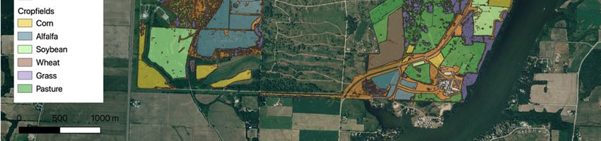
Sustainability 2020, 12, 765                                                                       2 of 21

aquatic systems [15–19], a major source for greenhouse gas release to the atmosphere [20,21] and a
large factor in soil degradation [12]. Livestock production, specifically dairy, has been identified as a
leading contributor to greenhouse gas emissions [22,23].
     Integrated crop–livestock systems (ICLSs) comprise a variety of practices that can reduce
greenhouse gas (GHG) emissions and water pollution [24] and enhance C-, N-, and P-cycling [25–27],
through appropriate fertilizer and manure applications. Practices may include grazing livestock on
crops and crop residues, planting forage cover crops, and trading animal waste and crop products
among farms [11,28]. ICLSs have greater potential to mimic the structure and function of natural
ecosystems [29–31], with less reliance on external inputs.
     In addition to decreasing GHG emissions of livestock, efforts to improve agroecosystem
sustainability may create new opportunities for income derived from on-farm production of ecosystem
services. However, estimating GHG budgets of farms can be challenging and is often accompanied
by large uncertainties, especially if no detailed knowledge about farm management practices are
available [32]. Life cycle assessments (LCA) using a variety of farm-scale models have been used to
understand greenhouse gas sources and to compare and contrast different dairy production systems of
varying extents (herd size and crop production acreage) [23]. However, these models range from simple
to highly complex interactions, may be highly regionally specific, and are often subject to extensive
calibration and validation [23]. Furthermore, the variability in landscape productivity is often ignored,
because it is particularly difficult to quantify in more complex terrain and landscapes [33]. Satellite
remote sensing techniques provide a cost-efficient way to significantly decrease data collection efforts
while simultaneously providing more information on vegetation productivity and emission variability
over time and space [34].
     To test this approach, here, we quantify ecosystem services provided by an ICLS in Wisconsin,
to understand how farm management affects environmental sustainability at different spatial and
temporal scales. For our first objective we evaluate the validity of quantifying the farm carbon sink
potential of the land base of a dairy farm in Wisconsin using satellite remote sensing techniques, by
comparing these with harvest totals for 2018. The novelty of this work compared to published work is
that this approach included the spatial and temporal estimation of ecosystem respiration, and gross
and net primary production (NPP) of carbon of the farm land cover—croplands and forest, shrub and
grassland vegetation—using remote sensing data. For our second objective, we evaluate the seasonal
and annual GHG offset potential of an ICLS farm in Wisconsin, by combining NPP estimates with
observations of emissions from enteric fermentation, and manure and field applications using the Tier
2 guidelines from the Intergovernmental Panel on Climate Change (IPCC).

2. Materials and Methods

2.1. Study Site
      The U.S. Dairy Forage Research Center (USDFRC) farm is located in Sauk County, Wisconsin,
USA. The climate is described as warm summer continental (Dfb, Köppen Climate Classification), with
a mean annual temperature of 8 ◦ C, receiving ~880 mm of precipitation per year. The majority of the
soils are characterized as being moderately well drained to excessively drained, with medium textured
soils over shallow quartzite rock outcroppings.
      The USDFRC farm (~890 ha), which operates jointly with the University of Wisconsin–Madison
College of Agricultural and Life Sciences, is located approximately 48 km northwest of Madison on
gently sloping acres bordering the Wisconsin River. The farm is a large-sized dairy for Wisconsin, with
approximately 400 dairy cows, in addition to heifers (1–24 months of age) and dry cows (~350). Crops
grown on the farm include corn for grain and silage, alfalfa for silage, soybeans and winter wheat
(Figure 1). The farm has several acres of open pasture used to graze heifers for approximately 6 months
each year. Livestock housing includes both tie-stall and free-stall barns. Cows are milked three times a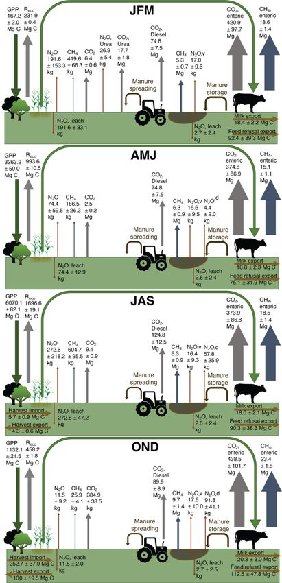
Sustainability 2020, 12, 765                                                                                             3 of 21

day. Cows in free-stall barns are fed from a total mixed ration (TMR) wagon. Average milk production
is approximately 13,150 kg (12,764 L) of milk per cow per year at 3.72% butterfat and 3.01% protein.
Sustainability 2020, 12, x FOR PEER REVIEW                                                     3 of 21

      Figure 1.
      Figure 1. Map
                Map of
                    of the
                       the Dairy
                           Dairy Forage
                                 Forage Research
                                        Research Center
                                                 Center and
                                                        and crop
                                                            crop field
                                                                 field compositions for 2018
                                                                       compositions for 2018 at
                                                                                             at Prairie
                                                                                                Prairie du
                                                                                                        du
      Sac, Sauk County,  WI.
      Sac, Sauk County, WI.

2.2. Meteorological Data
2.2. Meteorological Data
       A
       A weather
          weatherstation
                       stationinstalled   in January
                                   installed          2018 recorded
                                               in January             air temperature
                                                             2018 recorded                (using Onset,
                                                                                 air temperature           Inc. temperature
                                                                                                        (using    Onset, Inc.
sensor
temperature sensor S-TMB-M006 and relative humidity sensor S-THB-M006, attached to a Station,
         S-TMB-M006          and    relative  humidity   sensor   S-THB-M006,       attached    to  a  HOBO      U30     HOBO
Onset,   Inc., Bourne,
U30 Station,       Onset, MA,Inc., USA)    andMA,
                                     Bourne,     photosynthetic    active radiationactive
                                                     USA) and photosynthetic            (PAR) radiation
                                                                                                using a quantum
                                                                                                              (PAR) usingsensora
(HOBOnet       PAR    Sensor,     Onset,   Inc.  Bourne,   MA,    USA)   through    October
quantum sensor (HOBOnet PAR Sensor, Onset, Inc. Bourne, MA, USA) through October 2018. For     2018.    For    the remainder
of
thethe  year, we of
     remainder      obtained
                        the year, data
                                     wefrom    a weather
                                         obtained          station
                                                    data from       located in
                                                                 a weather       Necedah,
                                                                              station  locatedWisconsin,
                                                                                                 in Necedah,  approximately
                                                                                                                   Wisconsin,
100  km north of100
approximately         Prairie   du Sac.
                          km north     of Necedah
                                           Prairie duair temperature
                                                       Sac. Necedah air  and   PAR data were
                                                                            temperature           linearly
                                                                                             and PAR     dataregressed     with
                                                                                                                were linearly
data   collected   on   site  and   then  missing   data  for November      and  December
regressed with data collected on site and then missing data for November and December were gap-were    gap-filled    using  the
                                             DFRC = 0.7877            0.7877+× 19.54;    R =+0.9,   p < R0.05                 =
respective                                                   × DFRC                        2
filled usinglinear     regressionlinear
                the respective        (PARregression    (PAR    PAR=Necedah      PARNecedah     19.54;     2     & Tpair,DFRC
                                                                                                             = 0.9,    < 0.05 &
Tair,DFRC×=T0.8246
0.8246                 × T+0.8953;
              air,Necedah               R2 = 0.97,
                           air,Necedah +0.8953;   R2p=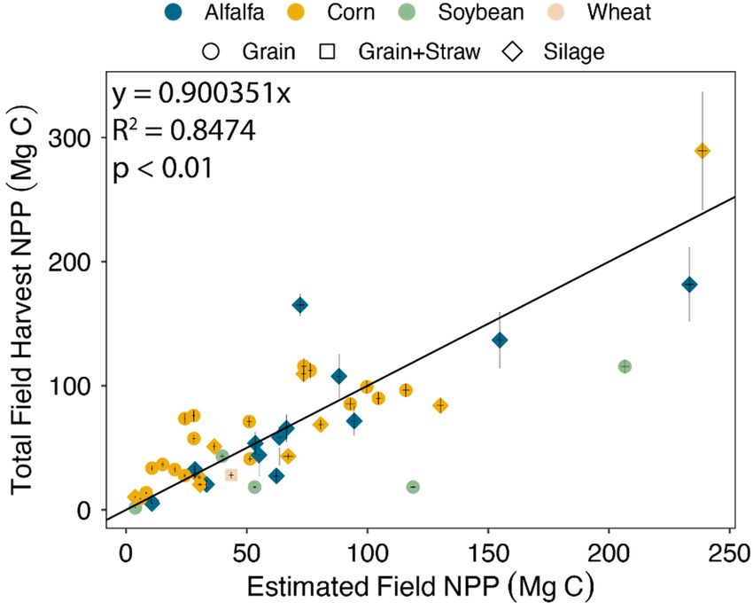
Sustainability 2020, 12, 765                                                                                   4 of 21

biomass as either all aboveground biomass was harvested for silage or residues were bailed and used
for silage or bedding on site.

      Table 1. Harvest data of dry matter (DM; %), harvest index (HI; %), proportion of root to aboveground
      biomass (in %), total aboveground biomass (kg), percent C, and estimated harvest, residual and root C,
      as well as their sum (whole plant C; kg C) for the crops of alfalfa, corn (dry, silage and high moisture
      corn (HMC)), winter wheat and soybeans, grown at Prairie du Sac dairy farm in 2018.

         Crop type              Alfalfa       Corn Silage      Dry Corn      HMC         Wheat       Soybeans
           DM (%)                  35             35              70           70          87            86
           HI (%)                  90             85              53           90          90            42
        Root from
                               120 (±30%)     21 (±30%)       21 (±30%)    21 (±30%)    90 (±30%)    19 (±30%)
     Aboveground (%)
    Total Aboveground
                               1,052,680.3    1,046,346.4      633,829.3    647,793.5   736,068.4     40403.2
       Biomass (kg)
            C (%)                  45             45              45           45          45            45
       Harvest C (kg)          468,969.1       466,147.3       282,371.0    288,592.0   139,116.9     17,999.6
       Residual C (kg)           4737.1         4708.6          2852.2       2915.1     192113.9       181.8
                               378,964.9       94,171.2        57,044.6     58,301.4    62,933.9       4181.7
         Root C (kg)
                                (±30%)         (±30%)          (±30%)       (±30%)      (±30%)        (±30%)
                               852,671.1       565,027.1       342,267.8    349,808.5   394,164.7     22,363.2
     Whole Plant C (kg)
                               (±16.4%)        (±5.2%)          (±5.2%)      (±5.2%)     (±8.6%)      (±4.8%)

2.4. Remote Sensing Gross Primary Productivity
     We obtained satellite data from Landsat 8 and the Moderate Resolution Imaging Spectroradiometer
(MODIS) for 2018 to estimate gross ecosystem productivity (GPP; g C m−2 ) using the satellite-based
Vegetation Photosynthesis model (VPM) developed by Xiao et al. [40]. Downscaled MODIS data
(from 250 by 250 m to Landsat 8 resolution of 30 m by 30 m) were used to gap-fill missing monthly
Landsat scenes (e.g., missing due to cloud obstruction or sensor failures). Because MODIS data have a
higher temporal resolution (1–8 days) the probability for cloud obstruction of particular scenes is lower
compared to Landsat 8 (16 days). The model simulates GPP using the enhanced vegetation index
(EVI), the land surface water index (LSWI) and land surface temperature (LST), as well as ground
observations of PAR. Landsat 8 EVI scenes (temporal resolution of 16 days) were directly downloaded
from USGS Earth Resources Observation and Science (EROS) Center Science Processing Architecture
(ESPA). EVI from Landsat and MODIS is estimated as follows:

                                                              (NIR − Red)
                                        EVI = 2.5 ×                                                               (1)
                                                       (NIR + 6 × Red − 7.5 × B + 1)

where NIR is the near-infrared band 5 (Landsat 8) and 2 (MODIS), Red the red band 4 (Landsat 8)
and 1 (MODIS), and B the blue band 2 on Landsat 8 and band 3 on MODIS. All Landsat scenes were
filtered using the quality assurance (QA) band (“pixel_qa”). MODIS EVI was estimated from raw
surface reflectance data, downloaded from ORNL DAAC using the MODIS/VIIRS subsets tool, which
were first filtered using the QC bands. Landsat LSWI, to describe liquid water contents in vegetation
canopies [41], was estimated from Landsat surface reflectance metadata, downloaded from USGS
EROS center, using the ToLSWI function of the rLandsat8 package in R. The function estimates LSWI as
follows:
                                               (NIR − SWIR1)
                                      LSWI =                                                       (2)
                                               (NIR + SWIR1)
where SWIR1 is the shortwave infrared band 6. For MODIS LSWI and EVI were estimated using the
lswi and evi functions in the water package in R, where SWIR is band 6 on MODIS satellites.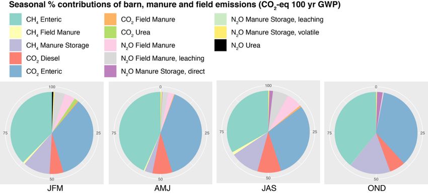
Sustainability 2020, 12, 765                                                                           5 of 21

    Landsat LST was estimated by first converting spectral radiance to brightness temperature
using the thermal constants provided in the raw Landsat metadata scenes and the function
ToAtSatelliteBrightnessTemperaure in the rLandsat8 package. Brightness temperature (BT) was then
converted to LST following the approach of Sobrino et al. [42]:

                                                            BT
                                       LST = h                           i                              (3)
                                                   1+λ×     BT
                                                             P   × ln(ε)

where P = h × cs = 14388 (um K−1 ), with h as the Planck constant (6.626 10–34 J s−1 ), s the Boltzmann
constant (1.38 10–23 J K−1 ) and c the velocity of light (2.998 10–8 m s−1 ). The parameter λ describes the
effective wavelength for the thermal bands, which is 10.6 for band 10 of Landsat 8. The parameter ε is
emissivity of the land surface, calculated using the Normalized Difference Vegetation Index (NDVI) to
describe the proportion of vegetation (PV) calculated as follows:
                                              "                            #2
                                            (NDVI − NDVImin )
                                      PV =                                                                (4)
                                           (NDVImax − NDVImin )

where NDVImin was assumed to be 0.2 and NDVImax 0.86 [42]. NDVI was estimated using the ToNDVI
function of the rLandsat8 package, which uses bands 4 (RED) and 5 (NIR) to calculate NDVI as
NDVI = (NIR − Red) / (NIR + Red). Emissivity (ε) was calculated as ε = εv ∗ PV + εs (1 − PV ) + 0.005,
where εv is vegetation emissivity (0.973) and εs soil emissivity (0.991) and 0.005 represents surface
roughness, here assumed to be constant [43]. MODIS LST (temporal resolution of 8 days) was
downloaded from ORNL DAAC using the MODIS/VIIRS subsets tool.
      The VPM model estimates GPP using PAR (as the sum for the 16 days surrounding Landsat or 8
days for MODIS scenes; see acquisition dates in Supplementary Information Table S1), the light use
efficiency for the different vegetation types (εg in g C mol−1 PAR), as well as EVI, LSWI and LST as
follows:
                                     GPPVPM = ε g × FPARchl × PAR                                  (5)

where FPARchl is the fraction of PAR absorbed by chlorophyll calculated as FPARchl = a × EVI, where
a = 1 following Xiao et al. [40,44] and Dong et al. [45]. The light use efficiency εg is derived from the
relationship of maximum quantum yield (ε0 ; g C mol−1 PAR; Supplementary Materials Table S2), taken
from literature values [46], scalars of temperature (Tscalar ) and water stressors to the vegetation (Wscalar
and Pscalar ) as follows:
                                     ε g = ε0 × Tscalar × Wscalar × Pscalar                              (6)

where Tscalar (0 > Tscalar < 1) is estimated as:

                                                  (T − Tmin )(T − Tmax )
                                Tscalar =                                    2                          (7)
                                            (T − Tmin )(T − Tmax ) − T − Topt

with Tmin , Tmax and Topt as the minimum, maximum and optimum temperatures for photosynthetic
activity, here set to be −1, 48 and 30 ◦ C for Wisconsin, respectively, according to [47] and T is LST from
Landsat or MODIS converted from K to ◦ C. When air temperature falls below Tmin , Tscalar is set to
0 [40]. Wscalar (0 > Wscalar < 1) is estimated as follows:

                                                          (1 + LSWI )
                                            Wscalar =                                                     (8)
                                                        (1 + LSWImax )

where LSWImax is the maximum LSWI within the growing season, set to 0.78 for 2018 in this study. The
scalar Pscalar is estimated as:
                                             (1 + LSWI )
                                   Pscalar =             .                                        (9)
                                                  2
Sustainability 2020, 12, 765 6 of 21
Each crop field and vegetation type (forest, shrub and grass) was assigned a ε0 (Supplementary
Materials Table S2) to generate a raster of maximum quantum yield.
Final GPP raster time series from Landsat were first gap-filled via the approxNA function from
the raster R package and then using GPP MODIS raster time series. The approxNA function estimates
missing pixel values through linear interpolation among time series of pixels from consecutive layers
(i.e., 16 day Landsat or MODIS GPP raster timeseries). For NA pixels in Landsat scenes, which could
not be filled using the approxNA function, we gap-filled data using a linear regression between Landsat
and downscaled MODIS pixels. Because MODIS GPP raster time series were 8 day products, we
first summed up 2 consecutive GPP raster products to match Landsat 16 day GPP raster timeseries
products. After that, MODIS pixel data were resampled from a cell resolution of 250 m by 250 m to
match the cell resolution of Landsat GPP rasters (30 m by 30 m) and to align cell centers among the
different products using bilinear interpolation. Bilinear interpolation uses the weighted average of
four nearest cells of the input raster to determine the cell value for the resampled output raster. We
then linearly regressed pixels of each Landsat GPP product with the respective MODIS product by
setting the intercept to 0 and thus obtaining a distinct slope (m) for each scene (Landsat GPP pixelx,y =
m × MODIS GPP pixelx,y , where x and y denote latitudinal and longitudinal coordinates). Landsat 8
raster pixels were then gap-filled using the respective linear regression for each timepoint.
2.5. Remote Sensing of Ecosystem Respiration
Spatial ecosystem respiration (Reco ) for the farm was estimated using a remote sensing model
developed by Gao et al. [48]. The model estimates Reco from GPP and crop biomass decomposition,
which depends closely on temperature. Reco (Equation 10) was calculated using a constant fraction
of GPP that is assumed to be spend on respiration (here a = 0.25, following Warring [49] and
Peichl et al. [50]; resembling a factor of NPP:GPP of 0.4–0.7), and a reference respiration rate (Rref ),
which was set to 2.86 g C m−2 for a reference temperature of 10 ◦ C (Tref ), estimated from eddy covariance
and soil respiration data (data not shown). Ecosystem respiration was then calculated as follows:
E0 × T 1 − 1
Reco = a × GPP + Rre f × e re f −T0 T−T0 (10)
where E0 is the temperature sensitivity of activation energy of respiration (263.59 K, converted to ◦ C),
estimated using the R package ReddyProc [51] and eddy covariance data of net ecosystem exchange of
CO2 which were available from the site from October 2018 through June 2019. The parameter T0 is the
minimum temperature for respiration (◦ C), which was set to −46.02 ◦ C, following Gao et al. [48] and
T is Landsat/MODIS Land Surface Temperature (◦ C). Similar to GPP calculations, we gapfilled Reco
timeseries via the approxNA function and then used resampled MODIS Reco raster time series to gapfill
Landsat NA pixels using a linear regression between Landsat and MODIS pixels.
2.6. Emission Inventories
2.6.1. Cattle Emissions
We obtained monthly herd inventory data from the dairy farm for 2018. Cattle were primarily
fed crops grown on site with the addition of protein mixes, lactation minerals, beet pulp molasses,
canola meal, calf starters, Geobond, and Reashure, depending on the cattle group. Dairy cows were fed
alfalfa silage (29.95%), corn silage (29.8%) high moisture corn (23.2%), roasted soybeans (7.4% of diet),
canola meal (8.3%), and lactation minerals (2.4%). Dry cows were fed corn silage (42.4%), grass hay
(20%), wheat straw (9.2%), canola meal (8.4), roasted soybeans (6.3%), HMC (4.5%), minerals (~2%)
and protein mixes (~2%). Heifers were fed a diet consisting of alfalfa silage (47%), corn silage (22.3%),
wheat straw (9.3%), and minerals (~1.5%) and special diets for calves (i.e., calf starter ~6%).
We obtained nutrient values for the diets from laboratory analysis for forage taken throughout the
year of 2018 (Dairyland; Table 2), and for TMR from the literature [52–54] for ingredients where noSustainability 2020, 12, 765 7 of 21
nutrient information was available (i.e., calf starters, canola meal, beet pulp and mineral additions).
Average nutrients by month and cow class were estimated using a weighted average, to account for
different percent contributions to each diet. Monthly manure emissions were then estimated following
Appuhamy et al. [55] by first calculating volatile solid excretion (VS; kg month−1 ) of all cattle on farm.
Volatile solids are biodegradable and nonbiodegradable fractions of organic matter in manure [55].
Monthly VS was calculated as a function of nutritional intake (Table 2):
VS = −1.201 + 0.402 × OMI + 0.036 × NDF − 0.024 × CP (11)
where OMI is organic matter intake (kg month−1 ), calculated as 85% from total monthly dry matter
intake (DM) for each cattle type (Table 2), CP (%) is crude protein and NDF (%) is non-digestible fiber,
both estimated as weighted averages for diets of each cow class.
Table 2. Average monthly nutritional dietary numbers and their standard deviations in parentheses by
cattle type (i.e., dairy, dry and heifers), where NC is the average monthly animal type count at the farm,
for dry matter intake (DM), volatile solid outputs (VS) and dietary nutrient values of crude protein
(CP), non-detergent fiber (NDF), dietary fats expressed as ether extract (EE), and ash (all in %).
Weight DM VS CP NDF EE Ash
Cow Type NC
(kg) (kg day−1 ) (kg Day−1 ) (% DM) (% DM) (% DM) (% DM)
14.9 31.4
Dairy 383 650(65) 22.2(8.6) 7.67 (1.26) 3.8 (0.26) 6.1 (1.00)
(0.92) (5.11)
30.3
Dry 53 680(68) 14.3(2.3) 4.90 (0.39) 9.3 (1.34) 2.0 (0.17) 6.1 (1.42)
(3.41)
16.3 40.1
Heifer 311 400(40) 6.0(2.6) 2.05 (0.19) 3.5 (0.20) 7.1 (0.94)
(2.02) (2.74)
Monthly feed refusal ranged from 5% to 12.5% of DM, similar to IPCC values. Feed refusal was
sold and thus treated as C leaving the farm boundaries. We estimated monthly enteric CH4 emissions
by different cattle groups following IPCC guidelines [38]:
Ym
GEI × 100
ECH4 , enteric = (12)
55.65
where Ym is the CH4 conversion factor (6.5 for dairy cows, 5.8 for dry cows and 3.0 for heifers). The
factor 55.65 is the energy content of methane and GEI is gross energy intake, calculated by multiplying
DM intake with gross energy (GE; Mcal kg−1 ), which was estimated from nutritional values of diets
fed to cattle following Weiss and Tebbe [56]:
GE = 0.045 × CP + 0.094 × EE + (100 − CP − EE − Ash) × 0.042 (13)
where EE is fat content (%) and Ash (%) is the total mineral content of a forage diet, expressed as
weighted average percentages of DM. The residual (100−CP−EE−Ash) was assumed to be mostly
polysaccharides [56]. Values of GE were converted to MJ kg−1 . Cattle CO2 emissions were estimated
from DM and average cow body weights (BW; Table 2):
ECO2 , enteric = −1.4 + 0.42 × DM + 0.045 × BW 0.75 (14)
2.6.2. Manure Emissions
Methane manure emissions (ECH4 ,manure ) were calculated following IPCC guidelines [38], where Bo
was the maximum methane producing capacity for dairy cows set at 0.24 for North America, MS was
the fraction of manure handled by the management system (in %). Due to manure field applications
during spring and fall, MS values were set at 90 (January, February, November, December), 50 (March,
August, September, October) and 10 (April–July). Monthly methane conversion factors (MCF;%)Sustainability 2020, 12, 765 8 of 21
for the liquid manure management system on site were set at 10 (January, February, December), 20
(March-May and November), and 30 (June-October) from IPCC guidelines [38]. Manure CH4 emissions
were estimated using total monthly VS inputs to the manure system as follows:
MS MCF
ECH4 ,manure = Bo × 0.67 × VS × × (15)
100 100
Nitrogen Oxide (N2 O) emissions from animal manure were estimated following IPCC Tier 2
guidelines [38] using DM intake and CP as:
CP
DM × 100
Nintake = . (16)
6.25
N excretion (Nexcretion ) was calculated using default values for nitrogen retention rates (Nret, f raction ;
kg N for 1000 kg animal mass day−1 ) for dairy cows in North America and estimates on N intake:
Nexcretion = Nintake × 1 − Nret, f raction (17)
where Nret, f raction was 0.2 for dairy cows and 0.07 for dry cows and heifers. Direct emissions were
estimated to be 0 during winter months, when average monthly temperature was below 0 ◦ C and a
factor EFN2 O of 0.005 (uncertainty of 0.01) was multiplied by Nexcretion , as direct emissions for spring,
summer and fall months while manure storage was liquid (with natural crust):
MS
EN2 O,manure = Nexcretion × × EFN2 O (18)
100
Finally, indirect emissions from volatilization to NH3 and NOx (EN2 O,vol ) and possible emissions
from N leaching (EN2 O, leach ) from the manure pit were estimated as follows:
44
EN2 O,vol = NC ∗ Nvol, f ract × EFN,vol × (19)
28
44
EN2 O, leach = NC ∗ Nleach, f ract × EFN,leach × (20)
28
where Nvol, f ract was 0.48 (for liquid/slurry manure storage), Nleach, f ract = 0.01, EFN,vol = 0.01 (assumed
to be minimal), and EFN,leach = 0.0075, as suggested by IPCC guidelines [38].
2.6.3. Field Emissions
Emissions from manure and fertilizer applications were estimated using data from the farm
nutrient management plan, which included liquid manure and bedding application by field, as well
as fertilizer applications like urea (on corn fields), diammonium phosphate and potassium chloride
(which were mainly applied on soybean and alfalfa fields). Urea contains approximately 20% carbon,
which was assumed to gas out completely within one week of application [38,57]. The carbon was then
converted to kg CO2 using the conversion factor of 44/12. For N2 O emissions from urea applications we
assumed a conversion factor of 0.00242 kg N2 O per kg of N applied. Urea applications only occurred
during spring months (March) in 2018.
2.6.4. C exports from Milk Production and Diesel Usage
Carbon exports from milk were estimated following Felber et al. [58] assuming that milk contains
20.8 ± 1.9 g C MJ−1 energy corrected milk (ECM; kg), adjusted to 3.14 MJ kg−1 based on Tyrell and
Reid [59]:
CM = (0.327 × milk) + (12.95 × f at) + (7.65 × protein) (21)Sustainability 2020, 12, 765 9 of 21
where milk, fat and protein were in kg, taken from 2 milk test days per month in 2018. Monthly milk
exports were estimated by multiplying daily bulk tank measurements (AgSource Dairy; Verona, WI,
USA) by the number of days in each month.
CO2 emissions from on-farm diesel use (from manure spreading, harvesting operations, etc.)
were estimated following Rotz et al. [60] assuming a conversion factor of 2.637 kg CO2 per liter of
diesel consumed. We did not treat diesel fuel as imported C, as we wanted to quantify its contribution
to the overall GHG budget of the farm and because we did not consider fuel as a stable carbon
storage product.
We converted all barnyard, manure, field and diesel emissions, as well as C exports from harvest
and milk (Supplementary Materials Table S3) to CO2 -eq (100 yr. greenhouse warming potential;
GWP) [61] to quantify if farm NPP for 2018 offset emissions from within the farm boundaries, as well
as to establish the source of emissions with the greatest impact on global warming [62]. Conversion
factors from the respective radiative forcing of an emitted gas reaching the atmosphere were 298 and
25 for N2 O and CH4 emissions, respectively [61].
2.7. Uncertainty Analysis
Uncertainty for remote sensing NPP was estimated by propagating GPP and Reco standard
deviations as follows: r
X 2
sdX = sdX,month (22)
where sdX is the mean annual (and seasonal) standard deviation estimated for X = GPP or Reco for
each crop field and natural vegetation type. We then calculated the annual (and seasonal) percent
error for NPP by averaging errors for GPP and Reco , respectively, using sdX divided by annual (and
seasonal) summed GPP and Reco . We estimated harvest NPP uncertainty by varying root fractions
by ±30%. Our confidence in HI and resulting residual data was high, thus excluded here from
uncertainty measurements.
Cattle diet nutrient intake and volatile solid output uncertainties were estimated using nutrient
variations from laboratory analyses of forage for CP, Ash, EE and NDF. In addition, we varied dry
matter intake by ±10% as the average uncertainty taken from feed refusal data, which was propagated
to VS outputs. These uncertainties were then propagated to CH4 and N2 O manure emissions, as well
as cattle CO2 and CH4 emissions, in addition to including standard deviations for feed dry matter (for
enteric CO2 ) and gross energy (for enteric CH4 ) intakes and body weights for each cattle group. For
direct N2 O emissions we also incorporated suggested uncertainties of ±50% from IPCC reports. For
volatile N2 O emissions from the manure pit we varied the fraction of volatile gas from 15% to 60%
for liquid manure as suggested by IPCC guidelines [38]. For N losses from leaching we varied the
fraction of leaching by ±10% [63]. For each calculation step we estimated the percent variability which
was then propagated to the next calculation step and finally to the parameter of interest (i.e., enteric,
manure and field emissions) for each month.
Uncertainty for C milk exports were estimated from fat, protein and milk energy content variations
taken from two milk test day results per month. Uncertainty was then propagated for each season
by also including the variability in C milk contents per milk energy content from Felber et al. [58].
Uncertainties for diesel emissions were assumed to be low and set at 10%, as purchase records
were available.
3. Results
3.1. Climate
Our study farm is located in a temperate mid-continental climate, with cold winters and warm,
wet summers. In 2018, average monthly air temperatures increased above 0 ◦ C in May, followed
by temperatures above 20 ◦ C from June through September (Supplementary Materials Figure S1).Sustainability 2020, 12, 765 10 of 21
Accumulated photosynthetic active radiation (PAR) for 16 days around the acquisition dates of Landsat
pictures was above 500 mol from March through the beginning of August, declining to 400–300 mol per
16 days from mid-August through the end of September. Annual rainfall amounted to approximately
1300 mm in 2018, which was ~400 mm higher compared to long-term records [64], with May and
August receiving the largest amounts with >200 mm of rain.
3.2. Net Carbon Budget
Prairie du Sac farm was a large carbon sink for 2018, where net primary productivity (NPP)
amounted to 7.25 million kg C (= 26.6 million kg of CO2 ; Figure 2), and total emissions (i.e., CO2 , CH4
and N2 O from manure, soil and cattle) were 6.69 million kg of CO2 -eq (Figure 3 and Supplementary
Materials Figures S2–S4). When expressed in area needed to offset farm emissions for ~750 dairy cattle,
the farm would need to produce either corn, alfalfa, soybeans or wheat on 2.97, 2.46, 2.92 or 3.0 km2 of
land, respectively, and the respective crop products would need to remain within the farm boundaries
Sustainability 2020, 12, x FOR PEER REVIEW 10 of 21
(Table 3). For natural vegetation either forests, shrub and grasslands would have to make up 2.82, 2.98
and 2.79 km2 to offset farm emissions, respectively. A farm with only pasture vegetation would require
up 2.82, 2.98 and 2.79 km2 to offset farm emissions, respectively. A farm with only pasture vegetation
2 km2 (~0.25 ha per 2cow) in size to offset emissions for 2018.
would require 2 km (~0.25 ha per cow) in size to offset emissions for 2018.
Figure 2. Correlation of estimated total annual sums of net primary productivity (NPP) from remote
Figure 2. Correlation of estimated total annual sums of net primary productivity (NPP) from remote
sensing data of cropfields versus harvest NPP. Harvest NPP was calculated from harvest indices and
sensing data of cropfields versus harvest NPP. Harvest NPP was calculated from harvest indices and
root:shoot ratios for alfalfa, corn, soybeans and winter wheat. Each point represents one field at Prairie
root:shoot ratios for alfalfa, corn, soybeans and winter wheat. Each point represents one field at Prairie
du Sac farm. Error bars on the x-axis represent standard deviations of NPP estimated for each cropfield
du Sac farm. Error bars on the x-axis represent standard deviations of NPP estimated for each
and on the y-axis propagated standard deviations for crop NPP, estimated by varying root:shoot ratios.
cropfield and on the y-axis propagated standard deviations for crop NPP, estimated by varying
root:shoot ratios.Sustainability 2020, 12, 765 11 of 21
Sustainability 2020, 12, x FOR PEER REVIEW 11 of 21
Figure 3. Seasonal
Seasonal schematics
schematics for
for C
C fluxes.
fluxes. C
C fluxes
fluxes represent
represent gross
gross primary
primary productivity
productivity (GPP)
(GPP) and
ecosystem respiration (Reco ),CCexports
eco), exportsfrom
frommilk,
milk,harvest
harvest and
and feed
feed refusals,
refusals, as
as well
well as
as greenhouse
greenhouse gas
gas
emissions from diesel (CO22,, Diesel)
Diesel) livestock
livestock (enteric fermentation of CO22,, enteric
enteric and
and CH44,, enteric),
enteric),
manure pit storage (CH44 and direct (N22O,O, d),
d), volatile
volatile (N22O,v)
O,v) and
and leached
leached (N(N22O,
O,leach)
leach) nitrogen
nitrogen oxide
oxide
emissions) and field (N2O, CH44 and
and COCO22emissions
emissionsfrom
from manure
manure and
and fertilizer
fertilizer applications). Seasons
Seasons
are separated by January, February, March (JFM), April, May, June (AMJ), July, August, September
(JAS) and October, November, December (OND).Sustainability 2020, 12, 765 12 of 21
Table 3. Annual Net primary productivity (NPP) by vegetation type, and estimated areas needed and
actual covered area of each vegetation type to offset annual greenhouse gas emissions from Prairie du
Sac dairy farm in 2018. The last column shows the area needed to offset emissions of one dairy cow (in
ha).
Area Needed to
Total NPP NPP Actual Area Area Needed
Vegetation Offset
(kg C) (kg C m2 ) Covered (%) per Cow (ha)
Emissions (km2 )
Alfalfa 1,217,208 0.77 2.46 64 0.33
Corn 1,364,220 0.64 2.97 72 0.40
Forest 923,831 0.67 2.82 49 0.38
Grass 1,867,659 0.68 2.79 99 0.37
Pasture 334,542 0.95 1.99 18 0.27
Shrub 626,255 0.63 2.98 33 0.40
Soybean 601,760 0.65 2.92 32 0.39
Wheat 317,883 0.63 3.01 17 0.40
3.3. Seasonal Greenhouse Gas Budget
Croplands were large C sources for the first three months in 2018, followed by forest, grass
and shrublands, whereas pastures were carbon sinks throughout all seasons (Supplementary
Materials Figure S4). Forest, grass and shrublands were the largest C sinks for April, May and
June months, whereas croplands sequestered more C during the months of July, August and September
(Supplementary Materials Figures S3–S5). Overall, perennial vegetation like pastures and alfalfa had
longer growing season and thus contributed to seasonal C sequestration more compared to annual
counterparts like corn or soybeans (Supplementary Materials Figure S3). Winter wheat fields were
only photosynthetically active from April through the end of July, when the crop started to senesce,
and seeds were ready to be harvested. Corn had sequestered the highest g C m−2 day−1 compared to
other vegetation types during July, when temperatures were highest, followed by alfalfa. Soybean
crops had low photosynthetic activity during early summer but were similar to corn and alfalfa fields
from the end of July through October. Photosynthetic activity and respiration at the farm were low
during winter months (December-February and March) when temperatures were below 0 ◦ C. Alfalfa
and corn were most productive, resulting in the highest biomass C accumulation of all crops harvested
at the site (Table 3). Soybeans and certain dry corn fields had the highest accumulation of residues,
whereas most crop fields had a harvest index (HI) of >0.9, leaving them mostly bare after harvest.
Estimated NPP (kg C) from Landsat/MODIS data fusion correlated well with calculated whole plant
NPP (kg C) from harvest data for each crop field (R2 = 0.85; p < 0.001; Figure 2), with greater variations
for corn fields. The farm, as a whole, was a carbon source (~13.6%; NPP of −0.064 Gigagrams) for the
first three months in 2018 (Figure 3) but sequestered more carbon during the rest of the year.
3.4. Seasonal Non-CO2 Sources and Carbon Imports and Exports
Emissions of N2 O, CH4 and CO2 from field manure applications (191 ± 153 kg direct N2 O
emissions, 192 ± 33 kg leached N2 O emissions, 420 ± 66 kg CH4 emissions, 6357 ± 636 kg CO2
emissions; Figure 3) and urea (2189 ± 438 kg N2 O and 4840 ± 484 kg CO2 ) application contributed
~11.2% to the overall CO2 -eq exports (2 ± 0.3 × 10⁶ kg) in January, February, and March (JFM), whereas
enteric CH4 and CO2 emissions exhibited 51.5% of all CO2 -eq exports (464,960 ± 34,872 kg CH4 and
420,920 ± 97,653.4 kg CO2 ). Manure emissions (132,067 ± 18,621) contributed 8% to the overall CO2 -eq
export, and feed refusal 19.7% (92,424 ± 39,262 kg C). Diesel emissions (74,866 ± 7487 kg CO2 ) and
milk C exports (18,410 ± 2190 kg C) were the smallest sources for CO2 -eq exports with 4.4% and 3.9%,
respectively (Figure 4).Sustainability 2020, 12, x FOR PEER REVIEW 13 of 21
Sustainability 2020, 12,±765
exports (18,410 2190 kg C) were the smallest sources for CO2-eq exports with 4.4% and133.9%,
of 21
respectively (Figure 4).
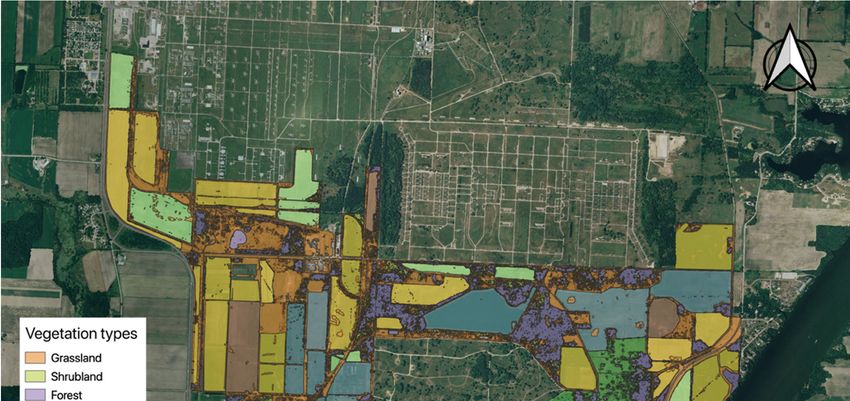
Figure 4. Percent contributions to total emissions of enteric fermentation, manure pit storage and field
Figure 4. Percent contributions to total emissions of enteric fermentation, manure pit storage and field
emissions of CO2 , CH4 and N2 O, expressed as 100 yr. CO2 -eq for each season in 2018. Seasons are
emissions of CO2, CH4 and N2O, expressed as 100 yr. CO2-eq for each season in 2018. Seasons are
separated by January, February, March (JFM), April, May, June (AMJ), July, August, September (JAS)
separated by January, February, March (JFM), April, May, June (AMJ), July, August, September (JAS)
and October, November, December (OND).
and October, November, December (OND).
For late spring and summer months (April, May and June, AMJ; Figures 3 and 4) enteric
For late (376,589
spring and summer
± 28,244 months (April, May and June, AMJ; Figures 3 and 4) enteric
fermentation kg CH 4 and 374,790 ± 86,951 kg CO2 ) contributed the majority
fermentation (376,589 ± 28,244 kg CH
to all farm CO2 -eq exports (1 ± 0.2 × 10⁶ kg) with± 58.8%,
4 and 374,790 86,951 followed
kg CO2) contributed the majority
by feed exports to all
with 21.5%
farm CO±2-eq
(75,046.0 exports
31,879.5 kg (1 0.2 ×10
C),± milk
6 kg) with
exports with 5.4%
58.8%, followed
(18,836.4 by feed
± 2338.4 kgexports
C) and with
diesel21.5% (75,046.0 ±
CO2 emissions
31,879.5 kg C), milk exports with 5.4% (18,836.4 ± 2338.4 kg C) and diesel CO 2 emissions of 5.9%
of 5.9% (74,866 ± 7487 kg CO2 ). Field manure and fertilizer applications (74 ± 60 kg direct N2 O
(74,866 ± 7487
emissions, kg kg
74 ± 13 COleached
2). Field manure and fertilizer applications (74 ± 60 kg direct N2O emissions, 74
N2 O emissions, 166 ± 26 kg CH4 emissions, 2498 ± 250 kg CO2 emissions)
± 13 kg leached N 2O emissions, 166 ± 26 kg CH4 emissions, 2498 ± 250 kg CO2 emissions) contributed
contributed 5.7% to all CO2 -eq exports, followed by manure emissions (2.6%; 26,685 ± 3763 kg CH4 ,
5.7% to all CO2-eq exports, followed by manure emissions (2.6%; 26,685 ± 3763 kg CH4, 1302 ± 583 kg
1302 ± 583 kg direct N2 O emissions, 4959 ± 2817 kg volatile N2 O emissions, 775 ± 713 kg N2 O manure
direct N2O emissions, 4959 ± 2817 kg volatile N2O emissions, 775 ± 713 kg N2O manure storage
storage leaching).
leaching).
In July, August and September (JAS; Figures 3 and 4), harvest imports from outside of the farm
In July, August and September (JAS; Figures 3 and 4), harvest imports from outside of the farm
property slightly counteracted overall C emissions (2 ± 0.3 × 10⁶ kg) by ~1.2%, but for October,
property slightly counteracted overall C emissions (2 ± 0.3 × 10⁶ kg) by ~1.2%, but for October,
November and December, farm imports lowered farm CO2 -eq exports by 50.9%. Nevertheless, farm
November and December, farm imports lowered farm CO2-eq exports by 50.9%. Nevertheless, farm
exports (mostly soybeans) added 0.9% and 20.2% in JAS and OND, respectively, to exports (2 ± 0.3 ×
exports (mostly soybeans) added 0.9% and 20.2% in JAS and OND, respectively, to exports (2 ± 0.3 ×
106 kg CO2 -eq). For JAS enteric emissions (18,490 ± 1387 kg CH4 and 373,923 ± 86,750 kg CO2 ) made
106 kg CO2-eq). For JAS enteric emissions (18,490 ± 1387 kg CH4 and 373,923 ± 86,750 kg CO2) made
up 46.3% of all CO2 -eq leaving the farm boundaries. N2 O and CH4 emissions from the manure pit
up 46.3% of all CO2-eq leaving the farm boundaries. N2O and CH4 emissions from the manure pit
(6295 ± 888 kg CH4 , 58 ± 26 kg direct N2 O, 16 ± 9 kg volatile N2 O and 3 ± 2 emissions from leached
(6295 ± 888 kg CH4, 58 ± 26 kg direct N2O, 16 ± 9 kg volatile N2O and 3 ± 2 emissions from leached
N2 O) and emissions from manure and fertilizer applications (273 ± 218 kg direct N2 O emissions,
N2O) and emissions from manure and fertilizer applications (273 ± 218 kg direct N2O emissions, 273
273 ± 47 kg N2 O leaching, 605 ± 96 kg CH4 and 9090 ± 909 kg CO2 ) contributed 10% and 14.9%,
± 47 kg N2O leaching, 605 ± 96 kg CH4 and 9090 ± 909 kg CO2) contributed 10% and 14.9%,
respectively. Diesel use (124,777 ± 12,478 kg CO2 ) amounted to 6.9% of the overall emissions, whereas
respectively. Diesel use (124,777 ± 12,478 kg CO2) amounted to 6.9% of the overall emissions, whereas
milk exports (18,044 ± 2148 kg C) accounted for 3.7% of the overall CO2 -eq export. Feed exports
milk exports (18,044 ± 2148 kg C) accounted for 3.7% of the overall CO2-eq export. Feed exports
(90,230 ± 38,330 kg C) were 18.3% of all CO2 -eq exports.
(90,230 ± 38,330 kg C) were 18.3% of all CO2-eq exports.
For October, November and December (OND; Figures 3 and 4), emissions from enteric fermentation
For October, November and December (OND; Figures 3 and 4), emissions from enteric
(23,379 ± 1754 kg CH4 and 438,524 ± 101,738 kg CO2 ) made up 54% of CO2 -eq exports, followed by
fermentation (23,379 ± 1754 kg CH4 and 438,524 ± 101,738 kg CO2) made up 54% of CO2-eq exports,
15% for manure pit (9696 ± 1367 kg CH4 , 92 ± 41 direct N2 O emissions, 18 ± 10 kg volatile N2 O and
followed by 15% for manure pit (9696 ± 1367 kg CH4, 92 ± 41 direct N2O emissions, 18 ± 10 kg volatile
2.7 ± 2.5 kg N2 O emissions from N2 O leaching) emissions and 21.9% from feed refusal (112,498 ±
N2O and 2.7 ± 2.5 kg N2O emissions from N2O leaching) emissions and 21.9% from feed refusal
47,789 kg C) exports. Milk C exports (20,347 ± 3008 kg C) contributed 4% and diesel CO2 (89,839 ±
(112,498 ± 47,789 kg C) exports. Milk C exports (20,347 ± 3008 kg C) contributed 4% and diesel CO2
8984 kg CO2 ) emissions 4.8% to all emissions. Field applications of manure and fertilizer (12 ± 9 kg
(89,839 ± 8984 kg CO2) emissions 4.8% to all emissions. Field applications of manure and fertilizer (12
direct N2 O emissions, 12 ± 2 N2 O emissions from leaching, 26 ± 4 kg CH4 , 385 ± 39 kg CO2 ) only
± 9 kg direct N2O emissions, 12 ± 2 N2O emissions from leaching, 26 ± 4 kg CH4, 385 ± 39 kg CO2) only
accounted for 0.6% of all emissions for OND.
accounted for 0.6% of all emissions for OND.Sustainability 2020, 12, 765 14 of 21
4. Discussion
4.1. Remote Sensing as a Tool for GHG Budget Estimation
Farm vegetation productivity is often derived from extensive field campaigns or, in more recent
cases, using eddy covariance measurements [65], which may impose challenges due to time or
funding constraints. Remote sensing techniques can significantly simplify this process at low cost [66].
Following objective one, we show that NPP estimated from remote sensing techniques gave exceptional
correlations with farm harvest data for individual crop fields.
Remotely sensed NPP correlated well with NPP calculated from annual harvest estimates by
field with greater variations for corn crops, likely due to differences in residue management for grain
and silage corn (Figure 2). Larger uncertainties existed for alfalfa harvest GPP, due to the lack of
belowground biomass data and greater variability in literature recorded root:shoot ratios. Overall
remote sensing technologies to estimate NPP can be used to simplify carbon budget accounting for
farms across the globe. Due to the relatively high resolution of Landsat images (30 by 30 m) farmers
can identify areas of low plant productivity, which could help to manage these areas using customized
nutrient management to increase productivity [67]. Alternatively, such areas could be converted to
pasture or grassland, to increase soil health and soil organic carbon (SOC) stocks. These practices could
further contribute to increase farm C sequestration, by improving crop yields, and offsetting GHG
emissions through plant biomass stocks [33].
4.2. Seasonal GHG Budgets and Recommendations for Reducing GHG Emissions on Dairy Farms
Following objective two, we show that the integrated crop–livestock farm in this study was a
large carbon sink on an annual basis. The farm could offset the majority of farm emissions through C
sequestered by farm vegetation. Specifically, natural vegetation like forests, shrub- and grassland offset
a large proportion of GHG emitted by the farm (Supplementary Materials Figure S4). Establishment
and active stewardship of natural vegetation cover, such as the forest cover, may therefore serve
as a potential mitigation strategy for dairy farm emissions [68]. The most vulnerable months for
GHG emissions at Prairie du Sac were winter and early spring months (i.e., JFM and OND) as plant
productivity was almost negligible when temperatures were low. For OND farm C exports made up
76% of C imports from plant productivity. Nevertheless, harvest inputs added ~18% to imported C,
thus decreasing the C emission balance of the farm. Trading harvest products could be an attractive
measure to offset farm emissions through interconnected farming systems, where farms serving as
large carbon sinks due to their extensive vegetation areas could serve as C donors through feed to
smaller farms, which may exceed their GHG budget on a seasonal or annual basis [69]. Similarly,
manure trading could increase farm sustainability [69], as field applications generally decrease GHG
emissions, specifically of CH4 due to less anaerobic conditions (Figure 3), compared to long-term
manure pit storage [70,71].
Our results show that there are a number of opportunities in feed, vegetation planting, and
manure management that can significantly lower GHG emissions on dairy farms while maintaining
production. Because pastures sequestered more carbon than they released back to the atmosphere even
during winter months, their integration into cattle diets, given that feed conversion efficiency remains
similar [71] at Prairie du Sac, could significantly lower the farm’s C emissions throughout the first
three months of the year (by at least 10%), compared to other crops. Furthermore, perennial vegetation
was shown to have lower overall soil GHG emissions compared to annual crops like corn [71], thus
further highlighting the GHG mitigation potential of pastures for dairy farms. Additionally, improving
field fertilizer and manure application strategies such as urea (here on corn fields) in conjunction
with urease inhibiters could significantly decrease N losses and N2 O emission from soils [72]. The
reduction in GHG emissions from ruminants fed with grains is therefore just one part of the picture, as
a more accurate accounting of emissions and milk production must include the C sequestered by feedSustainability 2020, 12, 765 15 of 21
crops [73]. Here, pastures had greater carbon uptake, highlighting the need to include farm practices
in development of GHG budgets [73].
Enteric fermentation (CH4 and CO2 ) made up the majority of GHG emissions at Prairie du Sac
farm, highlighting the importance of herd size and diet in shaping GHG budgets of livestock farms [74].
Dairy cows emitted the majority of CH4 and CO2 through ruminal fermentation, because their rations
were comparatively large with 22 kg DM, versus 14 kg and 6 kg for dry cows and heifers, respectively.
Herd size and composition directly affect GHG budgets, and dairy breeds like Jerseys may significantly
lower GHG emissions compared to Holsteins [75,76].
Even though the size of the farm land base allowed for high plant productivity, more diesel
was used to manage the farm landscape (i.e., manure applications, harvest, etc.), which resulted in
relatively large diesel CO2 emissions of 364 Mg CO2 annually. That number is equivalent to annual
GHG emissions of approximately 250 passenger vehicles (with an average emission rate of ~136 g
CO2 km-1 ) [77]. Reductions of such CO2 emissions could be accomplished through more efficient
manure transport and applications systems, like dragline systems [78,79]. Feed refusal C exports were
relatively large, thus a significant reduction in farm C exports could be accomplished through more
detailed feed intake knowledge of each individual cow and more controlled feed supply [80].
4.3. ICLSs for Managing Dairy GHG Emissions
Among GHG emission reduction practices, ICLSs may be one of the most sustainable approaches.
ICLS farms can serve as sustainable agroecosystems, especially when management practices increase
soil health and resilience to pests or weather extremes. Prairie du Sac ICLS farm was a large carbon
sink in 2018, even when C sequestration of natural vegetation from forests, shrub and grasslands was
excluded, highlighting the importance of on-farm product recycling in offsetting GHG emissions [81].
Grassland and pastures together could offset all farm emissions on site, whereas shrublands, corn,
wheat and soybean fields took up the least amount of carbon, due to their shorter growing season
(Supplementary Materials Figure S4), thus more area would be needed to offset farm emissions. Corn
and soybean production systems may also be unsustainable due to their impact on SOC losses [82], as
their root:shoot ratios are comparatively small [38], adding little to increase soil carbon stocks [69,83,84].
Furthermore, the management of corn fields at the Prairie du Sac dairy farm accumulated limited soil
C because residues left on site were negligible, as the majority of the crop biomass was chopped for
silage or baled for bedding following corn grain harvest. Alfalfa crops returned the highest amount of
C to the system compared to all crops grown on site, as their root systems are more extensive than
wheat, soybeans or corn crops. Perennials like alfalfa and pastures were productive earlier in the
season compared to soybeans and corn, as their persistence of living belowground biomass allowed
for more rapid leaf-out when temperatures were optimal [85]. Winter wheat, usually planted in the
fall of the previous year, also showed earlier photosynthetic productivity (Supplementary Materials
Figure S4). Nevertheless, earlier senescence of winter wheat plants (July) compared to alfalfa, corn and
soybeans decreased their carbon sink potential compared to other crops.
Integrated crop–livestock systems can offset more barn and manure emissions, as harvested
products remain within the farm boundaries [86]. In addition, pastures have a greater potential to
remain carbon sinks throughout all seasons, even when harvested for feed or bedding [73]. Natural
vegetation surrounding crop fields, such as forests, hedgerows or grasslands could offset farm emissions
even of non-integrated dairy farms, given that ~0.3–0.4 ha of such land is allocated per cow. The
largest C sources were attributed to enteric fermentation, especially of dairy cows, due to differences
in the nutritional composition of diets. Field and manure emissions were relatively low, showing
the importance of an adequate land base per animal for manure application as an important part of
ICLSs [9].Sustainability 2020, 12, 765 16 of 21
5. Conclusions
We show that remote sensing NPP provided an easy and cost-efficient way to estimate vegetation
productivity. This analysis can be implemented to estimate GHG budgets and describe milk production
not just in terms of animal efficiency but also in terms of environmental outcomes, thus giving a more
complete picture of the sustainability of livestock farms. ICLS farms have great potential to increase
agricultural sustainability, especially with strategic integration of perennial vegetation, as natural
vegetation like forest, shrub, grass and pasture productivity offset farm emissions and on-farm harvest
product recycling contributed to lower C exports. With a growing demand to feed an increasing
population, intensification of livestock agriculture, specifically dairy, has come at the cost of increasing
greenhouse gas emissions from unsustainable management practices [87,88]. Integrated crop–livestock
systems have the potential to offset farm greenhouse gas emissions, as crop C sequestration through
photosynthetic activity and plant biomass accumulation can offset GHG emissions produced within
the farm boundaries [86].
Even though remotely sensed NPP in this study showed good correlations with annual harvest
NPP, this research could be improved by including greater temporal and spatial resolution of remotely
sensed data (i.e., using hyperspectral drones). Greater resolution would allow for direct monthly
comparisons of vegetation productivity and changes in monthly GHG emissions of the barnyard. In
addition, in this study direct field measurements of cattle and field GHG emissions were not available
for 2018, therefore increasing the uncertainty around estimates, specifically regarding N2 O emissions.
Thus, for future work, field trials of monthly GHG soil emissions, particularly following manure and
fertilizer applications, as well as barn CO2 and CH4 emissions from enteric fermentation, should be
performed to reduce the uncertainty around these estimates.
Supplementary Materials: The following are available online at http://www.mdpi.com/2071-1050/12/3/765/s1,
Figure S1: Meteorological variables for the acquisition dates of Landsat surface reflectance products, Figure S2:
Estimated harvest net primary productivity by biomass component, Figure S3: Seasonal and spatial variations in
net primary productivity of carbon (NPP) for 2018 at DFRC dairy farm, Prairie du Sac, Figure S4: Total sums of
the carbon fluxes of gross primary productivity, ecosystem respiration and their sum net primary productivity
for each season of 2018, Figure S5: Daily sums of gross primary productivity of C of forest, pastures, shrub and
grasslands, as well as croplands, Table S1: Landsat and MODIS data availability for 2018, Table S2: Maximum
quantum yield data and area covered at Prairie du Sac dairy, and Table S3: Average monthly milk production at
the Dairy Forage Research Center dairy farm. Raw data of nutritional values for cattle diets, monthly cattle diet
compositions and field harvest and manure and urea applications are in process of being archived in USDA Ag
Data Commons (https://data.nal.usda.gov repository), DOI forthcoming prior to manuscript acceptance. In the
interim, reviewers may access data at https://github.com/susewuse/DFRC_GHG2018.
Author Contributions: S.W. and A.J.D. acquired data. S.W. calculated the carbon fluxes and emissions and
analyzed the data. A.R.D. helped with the calculation of remote sensing data. K.P.-B. helped with the statistical
analysis. All authors contributed to writing of this manuscript. All authors have read and agreed to the published
version of the manuscript.
Funding: This project was supported in part by an appointment to the Agricultural Research Services (ARS)
Research Participation Program, administered by ORISE through the U.S. Department of Energy Oak Ridge
Institute for Science and Education and the U.S. Department of Agriculture (USDA) Agricultural Research Services.
Any opinions, findings, conclusions, or recommendations expressed in this publication are those of the authors
and do not necessarily reflect the view of the U.S. Department of Agriculture.
Acknowledgments: We would like to thank the U.S. Dairy Forage Research Center and University of Wisconsin
staff for their hard work on the farm and for providing herd and feed inventory as well as harvest data.
Conflicts of Interest: The authors declare no conflict of interest.
References
1. Food and Agriculture Organization of the United Nations. FAOSTAT Statistical Database. FAO: Rome, Italy,
2019. Available online: http://www.fao.org/faostat/en/#data/QC (accessed on 25 July 2019).
2. Zhang, F.; Wang, Z.; Glidden, S.; Wu, Y.P.; Tang, L.; Liu, Q.Y.; Li, C.S.; Frolking, S. Changes in the soil organic
carbon balance on China’s cropland during the last two decades of the 20 th century. Sci. Rep. 2017, 7, 7144.
[CrossRef]You can also read