Stock Market Reactions to COVID-19 Pandemic Outbreak: Quantitative Evidence from ARDL Bounds Tests and Granger Causality Analysis
←
→
Page content transcription
If your browser does not render page correctly, please read the page content below
International Journal of
           Environmental Research
           and Public Health

Article
Stock Market Reactions to COVID-19 Pandemic
Outbreak: Quantitative Evidence from ARDL Bounds
Tests and Granger Causality Analysis
S, tefan Cristian Gherghina * , Daniel S, tefan Armeanu and Camelia Cătălina Joldes,
 Department of Finance, Bucharest University of Economic Studies, 6 Piata Romana, 010374 Bucharest, Romania;
 darmeanu@yahoo.com (D.S, .A.); joldes.catalina@yahoo.com (C.C.J.)
 * Correspondence: stefan.gherghina@fin.ase.ro; Tel.: +40-741-140-737

 Received: 5 August 2020; Accepted: 10 September 2020; Published: 15 September 2020

 Abstract: This paper examines the linkages in financial markets during coronavirus disease 2019
 (COVID-19) pandemic outbreak. For this purpose, daily stock market returns were used over
 the period of December 31, 2019–April 20, 2020 for the following economies: USA, Spain, Italy, France,
 Germany, UK, China, and Romania. The study applied the autoregressive distributed lag (ARDL)
 model to explore whether the Romanian stock market is impacted by the crisis generated by novel
 coronavirus. Granger causality was employed to investigate the causalities among COVID-19 and
 stock market returns, as well as between pandemic measures and several commodities. The outcomes
 of the ARDL approach failed to find evidence towards the impact of Chinese COVID-19 records on
 the Romanian financial market, neither in the short-term, nor in the long-term. On the other hand,
 our quantitative approach reveals a negative effect of the new deaths’ cases from Italy on the 10-year
 Romanian bond yield both in the short-run and long-run. The econometric research provide evidence
 that Romanian 10-year government bond is more sensitive to the news related to COVID-19 than
 the index of the Bucharest Stock Exchange. Granger causality analysis reveals causal associations
 between selected stock market returns and Philadelphia Gold/Silver Index.

 Keywords: COVID-19; stock market; ARDL model; Granger causality

1. Introduction
     With globalization, urban sprawl, and ecological transformations, contagious disease outbursts
turned out to be worldwide risks demanding a joint reply [1]. According to the International Monetary
Fund (IMF), coronavirus disease 2019 (COVID-19) generated an economic crisis different from
the others [2] for the reason that it is much more multifaceted (interconnections between the economy
and the health system), uncertain (the related treatment is established gradually, alongside the measures
concerning how to streamline isolation and the means to start over the economy), and has a worldwide
character. Both supply and demand reductions occur since individuals work and consume lower,
whereas companies diminish their productivity and investment [3]. Hence, Erokhin and Gao [4]
explored 45 developing states and established that food security status of individuals and the strength
of food supply chains are impacted by COVID-19.
     Consequently, governments have taken unprecedented actions, respectively fiscal measures
figuring to around $8 trillion, whereas central banks injected liquidity getting up to over $6 trillion [5].
The IMF has implemented exceptional measures by doubling its emergency loaning volume to
$100 billion and deferring debt outflows for poor nations [6]. Preparing for the economic recovery
raised a number of issues such as the way to maintain fiscal stimulus and unconventional monetary
policy, managing high unemployment, low interest rates, and preserving financial stability [7]. Hence,

Int. J. Environ. Res. Public Health 2020, 17, 6729; doi:10.3390/ijerph17186729   www.mdpi.com/journal/ijerph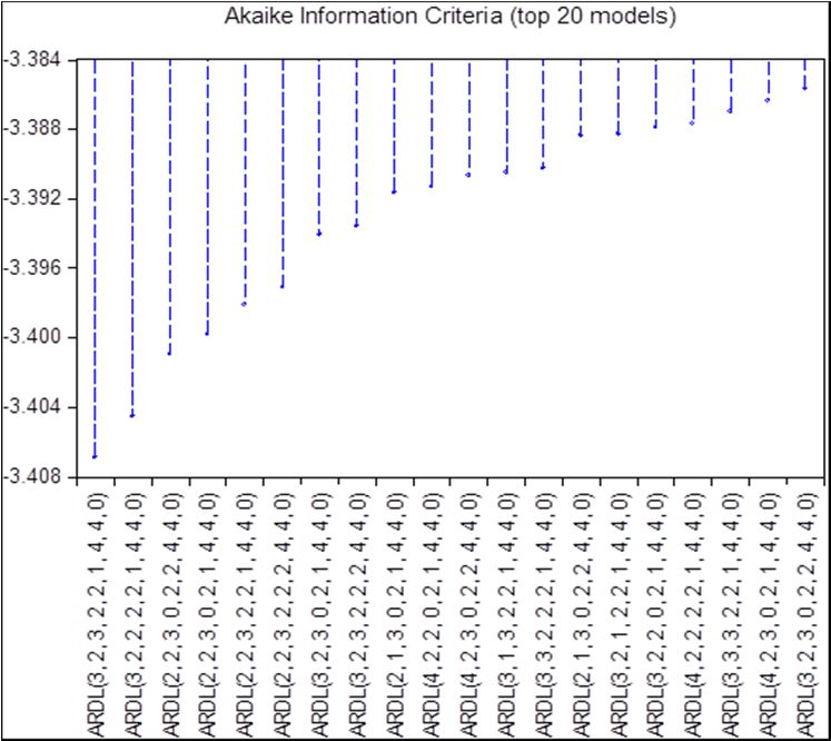
Int. J. Environ. Res. Public Health 2020, 17, 6729                                                     2 of 35

Narayan, et al. [8] exhibited that stimulus packages enhanced stock returns in Canada, UK, and USA,
but travel bans improved stock returns merely in Canada and Germany.
      The crisis caused by novel coronavirus severely limited broad economic activity [9].
Barro, et al. [10] contended that related economic failures are equivalent to those last registered
throughout the global Great Recession of 2008–2009. In a more pessimistic view, World Bank [11]
forecasted that the worldwide health crisis is driving the worst global recession since World War II.
Hence, Fernandes [12] estimated for 30 countries that a decline in gross domestic product of −2.8%
will occur in 2020. As well, Gormsen and Koijen [13] predicted that economic growth will decrease by
3.8% in the United States and by 6.3% in the European Union. Likewise, Estrada, et al. [14] claimed
that the potential growth of China would be reduced by 0.45%, respectively an undesirable impact of
about three times higher than the outcome of Severe Acute Respiratory Syndrome (SARS).
      COVID-19 is an emblematic black swan case, its incidence, expansion, and dissolution, as well
as the complexity, range, and strength of its influence, are all indefinite [15]. Thus, the substantial
insecurity of the outbreak and its related economic damages has entailed markets to become extremely
unstable and changeable [16]. On March 16, 2020, Chicago Board Options Exchange Volatility Index
(VIX) closed at the uppermost level since its inauguration [17]. Gold registered the highest level since
January 2013 [18], but has been particularly variable since mid-February [19]. Nevertheless, the safe
haven standing of gold vanished during corona crisis because its prices shifted in tandem with the stock
markets of the ten largest economies [20,21]. As well, on April 20, 2020, traders tried to avoid physical
possession of oil and massively sold oil futures contracts, sending them into negative region for the first
time in history [22]. Salisu, et al. [23] found that a 1% drop in crude oil price returns rises the likelihood
of registering undesirable stock returns before the pandemic proclamation. Consequently, there was
acknowledged that the coronavirus pandemic has weakened oil demand and there is not enough
storage space for overproduction of oil in the United States (for instance, nearly 85% of global onshore
storage was filled) [24]. Investors liquidated the May futures contracts that matured on Tuesday (April
21, 2020), the price of West Texas Intermediate (WTI) oil registering the value of –37.63 dollars/barrel,
at the end of the day [25].
      Recent studies focused on the impact of coronavirus on various measures such as exchange
rate [26], financial volatility [27,28], stock returns [29–34], corporate bonds [35] or Eurobonds [36], oil
price [37], or economic policy uncertainty [38], alongside employing various methods towards assessing
the diffusion of the virus [39,40] or assessing the source of health security [41,42]. We contribute to this
growing literature by exploring the associations in stock markets throughout COVID-19 pandemic
outbreak. First, we explore whether the Romanian stock market is impacted by the crisis generated
by novel coronavirus. To the best of our knowledge, this is the first study addressing the impact of
COVID-19 from both China and Italy on the Romanian capital market and the 10-year Romanian
bond. Nations in Eastern Europe have circumvented huge virus occurrences than those registered
in other parts of the continent [43] such as Italy, United Kingdom, Spain, or France. Nonetheless,
Romania is one of the most affected country in the region since many of its citizens get back from Italy
and Spain [44]. Many developing nations depending on overseas revenue in form of a mixture of
commodity exports, tourism, and remittances are expected to fail due to liquidity scarcity and lack
of tax revenues [45]. Eissa [46] highlighted disparities in health expenditures per capita, the highest
levels being registered in North America and Western Europe, but the lowest in West, Central, and East
Africa. Although remarkable fiscal-budgetary instruments have been implemented by many European
governments (e.g., 50 per cent of GDP in Italy, 28 per cent in Germany, 19 per cent in France, 12 per
cent in Poland, 11 per cent in Spain, 6.5 per cent in Serbia), Romania ensured a fiscal assistance of just
3.5 per cent of GDP [47]. Secondly, our research investigates the causalities among COVID-19 and
major stock market returns, as well as between pandemic measures and several commodities.
      The rest of this manuscript proceeds as follows. Section 2 reviews prior studies. Section 3 discusses
the sample and quantitative methods. Section 4 focuses on empirical outcomes. Final section presents
the conclusions and the main policy implications.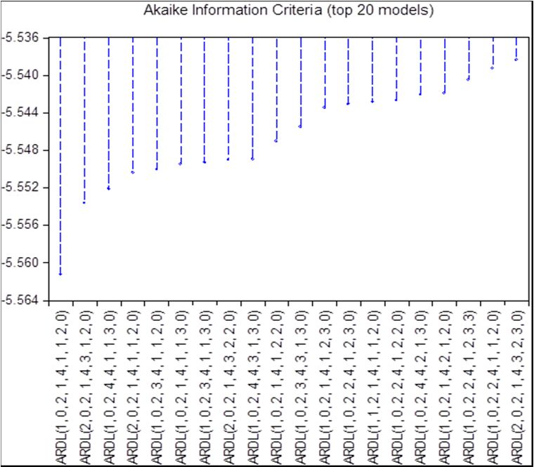
Int. J. Environ. Res. Public Health 2020, 17, 6729                                                  3 of 35

2. Related Literature

2.1. Prior Research Regarding the Economic and Financial Consequences of COVID-19
     The COVID-19 contagion triggered a failure in worldwide stock markets resulting in
an unpredictable setting with critical liquidity levels [48]. Therewith, substantial contagion between
nations was noticed by Hafner [49] attributable to noteworthy serial and spatial autocorrelations.
Giudice, et al. [50] noticed that current pandemic affected housing values, whereas Babuna, et al. [51]
emphasized that insurance industry registered losses.
     Beck, et al. [52] investigated ten emerging markets and found that most of companies were
harmfully influenced by COVID-19, whereas Haroon and Rizvi [53] explored 23 emerging markets
and provided support that reducing (growing) course of coronavirus cases is related with enhancing
(worsening) liquidity in financial markets. In a similar vein, Baig, et al. [54] claimed that community
panic, alongside constraints and quarantine drive the cash shortage and uncertainty of the markets.
Erdem [55] investigated stock market indices of 75 nations and supported that markets are negatively
influenced by the pandemic. Therefore, the coronavirus health calamity switched into a wider economic
and financial disaster [56], marked by decline in business profitability and employment, alongside
an upsurge in debt [57]. To these concerns are added the ongoing challenges like stimulating trade,
fintech, digital transformation, and combating climate change.
     Since the SARS-CoV-2 virus is spreadable and migrations occurs, current pandemic outbreak affect
many nations worldwide, along with their stock markets [58]. Hence, Shehzad, et al. [59] documented
that conditional variance of stock markets from Europe and USA is huge throughout the period of
COVID-19 as related to the Global Financial Crises (GFC) of 2007–2009. Estrada, et al. [60] explored ten
major stock markets worldwide and cautioned that the effects of SARS-CoV-2 crisis may engender
comparable impairment of the Crisis 1929, also being estimated a period between 9 and 12 months
for recovery. Mishra, et al. [61] revealed that all Indian stock market returns were negative during
COVID-19 as compared with contemporary main structural changes such as demonetization and
implementation of goods and services tax. In contrast, Bhuyan, et al. [62] exposed that stock market
returns of the SARS diseased nations displayed substantial rise related to the pre-SARS stage. Baltussen
and Vliet [63] concluded that through the recovery period in the aftermath of Spanish Flu contagion
small caps showed the strongest performance. Likewise, Ding, et al. [64] revealed that stock price
decrease was lesser for companies showing pre-2020 funds, with a minor contact with the virus over
international supply chains and clients places, many corporate social responsibility (CSR) actions, and
fewer entrenched directors. Singh [65] argued that investors are focused on environmental, social, and
governance (ESG) portfolio since it centers on the long-term sustainability of corporations. In addition,
Palma-Ruiz, et al. [66] documented for a sample of 35 IBEX-35 companies that investors are more
oriented towards ESG features. Therefore, Pástor and Vorsatz [67] recommended funds with high
sustainability ratings, suggesting the opinion that sustainability is a requirement instead of opulence.
     The occurrence of SARS-CoV-2 virus influenced the economic setting and marked investor
sentiment, also triggering stock price fluctuations [15]. Yilmazkuday [68] exhibited that an upsurge
in daily total fatalities due to SARS-CoV-2 will lessen the international economic activity assessed
through by the Baltic Exchange Dry Index. Ru, et al. [69] claimed that investors from nations with prior
knowledge of comparable calamities respond more quickly to COVID-19 than the investors deprived
of experience. Hassan, et al. [70] suggested that firms having experience with SARS or H1N1 own
more positive prospects towards their capacity to handle the SARS-CoV-2 epidemic.
     As regards investing strategies over the SARS-CoV-2 crisis, Ortmann, et al. [71] suggested that
investors open more stock and index positions, but do not shift to safe-haven or perilous investments.
Hence, Cheema, Faff and Szulczyk [20], Cheema, Faff and Szulczyk [21] advised that gold and
silver lost momentum in favor of liquid and stable assets such as treasuries and the Swiss franc.
Mensi, et al. [72] proved that gold and oil turned out to be more inefficient throughout the corona crisis
related to the pre-pandemic period. Hence, investors can establish profitable approaches by exploiting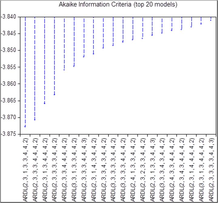
Int. J. Environ. Res. Public Health 2020, 17, 6729                                                    4 of 35

market inefficiencies to acquire abnormal returns [73]. On the contrary, Yan, et al. [74] recommended
the tourism industry, technology sector, leisure industry, and gold as suitable investments. Li, et al. [75]
endorsed health sector in line with Chong, et al. [76] which suggested over SARS to buy medical stocks
and sell tourism stocks. In terms of cryptocurrencies, Chen, et al. [77] argued that augmented concerns
of the coronavirus caused negative Bitcoin returns and large trading volume, whereas Conlon and
McGee [78] advised that it does not perform as a hedge.
      With reference to the influence of the pandemic on the enterprise’s activities, Mazur, et al. [79]
contended that companies reply in various means to the COVID-19 revenue shock because many sectors
were locked throughout the quarantine stage. Hence, Xiong, Wu, Hou and Zhang [9] evidenced that
companies belonging to sectors that are exposed to the pandemic have significantly lower cumulative
abnormal returns, but enterprises with good financial conditions endure less opposing effect of
the disease. Nguyen [80] established that energy segment experienced the utmost abnormal negative
returns amid all sectors. Fallahgoul [81] established that the financial segment is the most doubtful,
whereas health is the most hopeful over the COVID-19 pandemic. He, Sun, Zhang and Li [15] claimed
that manufacturing, information technology, education and health-care Chinese sectors remained
stable to COVID-19. Gu, et al. [82] found that Chinese manufacturing sector was hardly hit by corona
crisis, but construction, information transfer, computer services and software, and health care and
social work were positively influenced by COVID-19.

2.2. Earlier Studies towards the Impact of COVID-19 on Stock Markets
      Financial markets worldwide confronted with the flight-to-safety phenomenon which engendered
a severe deterioration in asset appraisals and amplified volatility around the world [11]. Baker, Bloom,
Davis, Kost, Sammon and Viratyosin [30] stressed that there was no prior illness that determined such
daily stock market jumps. Albulescu [83] emphasized that the fatality rate has a positive and very
significant influence on financial volatility, whereas Albuquerque, Koskinen, Yang and Zhang [31]
found that green stocks are highly valued and register lower volatility and larger trading volumes
than the rest of stocks.
      Markets are a function of government, hence responding reliant on authority reply [84]. Alfaro,
Chari, Greenland and Schott [32] confirmed that a doubling of projected contaminations is linked with
a 4 to 11 percent deterioration of aggregate market value. Alber [85] showed that stock market return is
influenced by COVID-19 cases more than deaths, as well as by aggregate measures more than new ones.
However, attributable to local features, the influence of novel coronavirus may diverge across equity
markets [86]. Onali [33] revealed that variations in the amount of cases and deaths in the USA and
other highly impacted nations by the coronavirus do not influence stock market returns out of USA,
except the number of cases for China. The spread of COVID-19 globally driven an upsurge of yields
on sovereign securities more than proportionally in developing and emerging states [36]. Nozawa
and Qiu [35] noticed that corporate bonds supplied by companies showing a strong link with China
respond more to the quarantine of Wuhan at early 2020. Hence, M.Al-Awadhi, Alsaifi, Al-Awadhi
and Alhammadi [29] concluded that the COVID-19 disease negatively influence stock market returns
of the companies covered in the Hang Seng Index and Shanghai Stock Exchange Composite Index.
Adenomon, Maijamaa and John [34] strengthened that the coronavirus disease negatively influences
the stock returns in Nigeria.
      On the contrary, there was proved that everyday cases of new contagions have a low adverse effect
on the crude oil quotations in the long-term [37]. Albulescu [38] explored whether the COVID-19 and
crude oil influence the economic policy uncertainty of the United States and observed no impact when
considering the global coronavirus data, but a positive effect when assessing the condition outside
China. Sharif, et al. [87] established a unique responsiveness of stock market of USA, related economic
policy uncertainty, and geopolitical risk to the joint shocks of the coronavirus and oil instability. For
the case of Colombia, Cardona-Arenas and Serna-Gómez [26] argued that the depreciation of national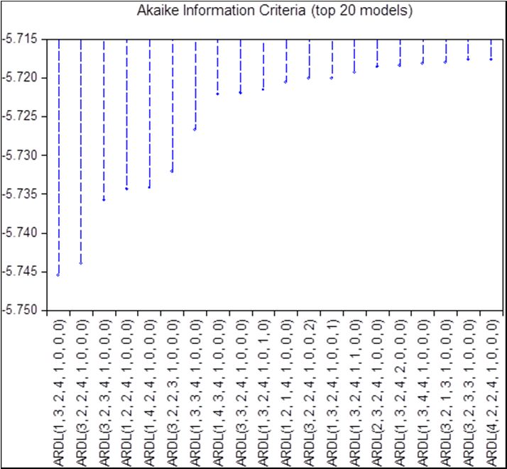
Int. J. Environ. Res. Public Health 2020, 17, 6729                                                              5 of 35

currency against the dollar commenced after the diagnosis of the initial positive coronavirus case
which determined a rise in global oil value.
     Pavlyshenko [39] argued that varied turmoil exerts distinct influence on the similar assets. Hence,
Mamaysky [88] exhibited that VIX is most Granger caused by the news even if the other asset kinds
are also Granger caused by the news.
     Due to reduced level of economic growth and deficiency of capital influxes, emerging markets
show inadequate funds to handle the pandemic and thus are likely to undergo worst [86]. Hence, we
postulate the following research hypotheses:

Hypothesis 1 (H1). The stock market index of the Bucharest Stock Exchange is negatively affected by the number
of new cases and new deaths due to COVID-19 in China and Italy.

Hypothesis 2 (H2). The Romanian 10-year bond yield is negatively affected by the number of new cases and
new deaths due to COVID-19 in China and Italy.

3. Empirical Framework

3.1. Sample and Variables
     Daily stock market returns over the period 31 December 2019–20 April 2020 were collected for
the following economies: United States (USA), Spain (ES), Italy (IT), France (FR), Germany (DE),
United Kingdom (UK), China (CH), and Romania (RO). The selected measures are depicted in Table 1.
Alike Lyócsa, et al. [66], the timespan was selected since over the beginning of the corona disaster,
the value of the market dropped, whereas insecurity in the market amplified severely.

                                                 Table 1. Variable descriptions.

           Variables                                   Description                               Source
                                    Variables towards COVID-19 pandemic outbreak
            NC_CH               The number of new cases due to COVID-19 in China            Our World in Data
           ND_CH                The number of new deaths due to COVID-19 in China           Our World in Data
            NC_IT                The number of new cases due to COVID-19 in Italy           Our World in Data
            ND_IT               The number of new deaths due to COVID-19 in Italy           Our World in Data
                                         Variables concerning stock market returns
                                  The daily percentage change of close price of Dow
            DJIA_R                                                                        Thomson Reuters Eikon
                                           Jones Industrial Average (USA)
                                The daily percentage change of close price of S&P 500
                                  (USA). The S&P 500 is usually viewed as the best
            SPX_R                single gauge of large-cap U.S. equities. The index       Thomson Reuters Eikon
                                consist of 500 leading corporations and covers about
                                        80% of existing market capitalization
                                The daily percentage change of close price of IBEX 35
                                  (Spain). The IBEX 35 index is intended to denote
                                    real-time progress of the most liquid stocks in
          IBEX35_R                    the Spanish Stock Exchange and for use as           Thomson Reuters Eikon
                                     an underlying index for trading in financial
                                derivatives. It is composed of the 35 securities listed
                                                on the Stock Exchange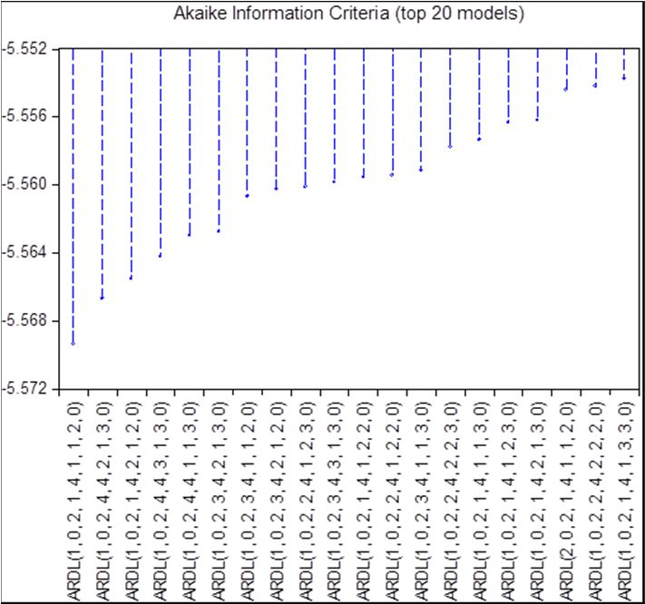
Int. J. Environ. Res. Public Health 2020, 17, 6729                                                             6 of 35

                                                           Table 1. Cont.

           Variables                                     Description                            Source
                                 The daily percentage change of close price of FTSE
                                MIB (Italy). The FTSE MIB is the benchmark index for
           FTMIB_R                  the Borsa Italiana, the Italian National Stock       Thomson Reuters Eikon
                                Exchange and covers the 40 most-traded stock classes
                                                   on the exchange
                                The daily percentage change of close price of CAC 40
                                 (France). The CAC 40 is a benchmark French stock
                                         market index. The index represents
            FCHI_R                                                                       Thomson Reuters Eikon
                                  a capitalization-weighted measure of the 40 most
                                significant stocks among the 100 largest market caps
                                  on the Euronext Paris (formerly the Paris Bourse)
                                The daily percentage change of close price of DAX 30
                                  (Germany). The DAX is a blue-chip stock market
          GDAXI_R                                                                        Thomson Reuters Eikon
                                index comprising the 30 major German corporations
                                      trading on the Frankfurt Stock Exchange
                                 The daily percentage change of close price of FTSE
                                  100 (UK). The Financial Times Stock Exchange 100
            FTSE_R               Index is a share index of the 100 corporations listed   Thomson Reuters Eikon
                                   on the London Stock Exchange with the highest
                                                 market capitalization
                                The daily percentage change of close price of SSE 100
                                  (China). SSE 100 Index consists of 100 stocks with
                                features of most rapid operating income growth rate
           SSE100_R              and highest return on equity within the universe of     Thomson Reuters Eikon
                                    SSE 380 Index, and aims to reflect the overall
                                performance of core stocks in the emerging blue chip
                                        sector that trade in Shanghai market
                                  The daily percentage change of close price of BET
                                (Romania). Bucharest Exchange Trading Index (BET)
            BET_R                                                                        Thomson Reuters Eikon
                                   is a capitalization weighted index, comprised of
                                   the 10 most liquid stocks listed on the BSE tier 1
                                               Variables regarding commodities
                                 Cushing, OK Crude Oil Future Contract 1 (Dollars         Energy Information
         CRUDE_OIL
                                                  per Barrel)                               Administration
                                                                                          Energy Information
              WTI               Cushing, OK WTI Spot Price FOB (Dollars per Barrel)
                                                                                            Administration
                                 Natural Gas Futures Contract 1 (Dollars per Million      Energy Information
      NATURAL_GAS
                                                       Btu)                                 Administration
                                The New York Mercantile Exchange (NYMEX) Light
             LSCO                                                                        Thomson Reuters Eikon
                                            Sweet Crude Oil (WTI)
                                     The daily percentage change of close price of
            XAU_R                                                                        Thomson Reuters Eikon
                                           Philadelphia Gold/Silver Index
                                                Variables regarding currencies
          EUR_CNY                     The daily percentage change of EUR/CNY                 Investing.com
                                 Variables regarding 10-Year Government Bond Spreads
                                The daily percentage change of the Romanian 10-year
          RO_BOND                                                                            Investing.com
                                                     bond yield
                                                     Source: Authors’ own work.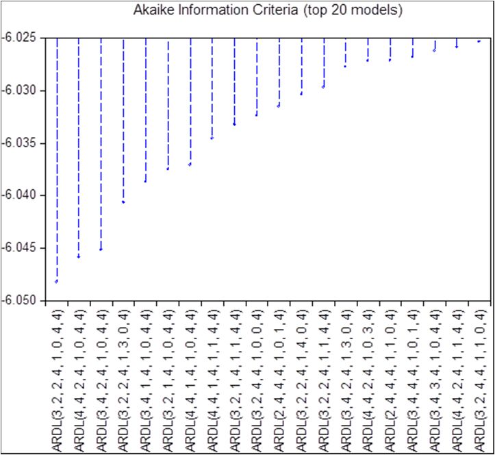
Int. J. Environ. Res. Public Health 2020, 17, 6729                                                  7 of 35

   In addition, we have included a wide range of variables that allow us to achieve our goal, such as
COVID-19 measures, commodities, currencies, and 10-Year government bond spreads.

3.2. Quantitative Methods
     In order to gain insights towards the linkages in stock markets during COVID-19 pandemic
outbreak, we will use the autoregressive distributed lag (ARDL) model similar Albulescu [37,38],
Erokhin and Gao [4], as well as Granger causality test alike Mamaysky [88]. Checking for unit root in
ARDL approach is not fundamental in as much as it can examine for the occurrence of cointegration
among a set of variables of order I(0) or I(1) or a mixture of them. Hence, the leading benefit of ARDL
model consist in its versatility. However, the ARDL methodology impose that no variable should be
integrated of second order or I(2). Therefore, in line with prior research [26,34,59], the augmented
Dickey–Fuller (ADF) test will be applied for unit root testing. The null hypothesis of the ADF test
claims the presence of unit root in the time series.
     The ADF test involves estimating the following equation:
                                                        Xk
                               ∆ωt = α + βt + qωt +              γj ∆ωt−j + εt , t = 1, . . . , T      (1)
                                                           j=1

where t denotes the time trend, T signifies the length of the sample, while k is the length of the lag in
the dependent variable.
     Further, ARDL model examines the long and short-term cointegration, being specified as a sole
equation framed with adaptable choice of lag extents. The general form of an ARDL (p, q) model is as
follows:
               Wt = µ + β0 Zt + β1 Zt−1 + · · · + βq0 Zt−q + δ1 Wt−1 + · · · + δp Wt−p + ut           (2)

     The lag orders p and q are established by means of the Akaike Information criteria and may differ
over the explanatory variables covered in our quantitative framework.
     The Granger causality test can be applied to analyze the causality between variables, as in
Mamaysky [88]. The null hypothesis is that w does not Granger-cause z and that z does not
Granger-cause w. The following bivariate regressions will be estimated:

                           zt = α0 + α1 zt−1 + · · · + αp zt−p + β1 wt−1 + · · · + βp w−p + t         (3)

                          wt = α0 + α1 wt−1 + · · · + αp wt−p + β1 zt−1 + · · · + βp z−p + ut          (4)

4. Econometric Findings

4.1. Summary Statistics, Correlations and Stationarity Examination
      The descriptive statistics of the variables are provided in Table 2. The distributions of all stock
market returns, as well as most of included commodities are negatively skewed. Thus, negative returns
are more prevalent than positive returns, supporting a greater likelihood for very high losses. Kurtosis
shows the thickness of the tail and highlights a high level of risk for selected stock markets, especially
Spain and Italy. In addition, except EUR/CNY and Natural Gas Futures Contract 1, the Jarque–Bera
test provides evidence that selected series are not normally distributed.
      Figure 1 shows the evolution of the number of new cases due to COVID-19, whereas Figure 2
reveals the progress of the number of new death due to COVID-19. There is noticed that USA registers
the highest figures in this regard.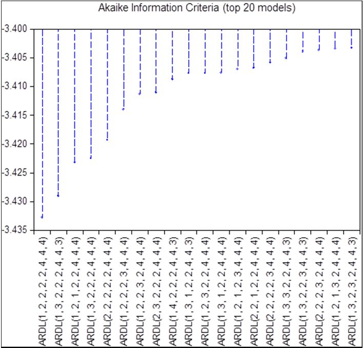
Int. J. Environ. Res. Public Health 2020, 17, 6729                                                                                                                              8 of 35

                                                                           Table 2. Descriptive statistics of the variables.

                                                                                        Standard
                         Variables                   Mean            Median                                  Skewness             Kurtosis          Jarque–Bera   Probability
                                                                                        Deviation
                         NC_CH                   887.5000             98.5000            2040.816               5.02                34.31               3243.22      0.00
                         ND_CH                    33.0278             10.5000             47.9956              2.13                 8.31                 138.78      0.00
                          NC_IT                  1521.139             95.0000            1934.999              0.78                 1.99                  10.45      0.01
                         ND_IT                   208.0139             4.5000             279.6809               0.85                2.06                 11.23       0.00
                         DJIA_R                  −0.002321             0.0000              0.0371              −0.39                 5.89                 2.88       0.00
                          SPX_R                   −0.0024              0.0001              0.0341              −0.67                 5.76                28.26       0.00
                       IBEX35_R                   −0.0052             −0.0008              0.0301              −1.69                10.65                210.03      0.00
                        FTMIB_R                   −0.0052              0.0013              0.0337              −2.53                14.67                485.29      0.00
                         FCHI_R                   −0.0038              0.0003              0.0299              −1.16                 7.51                77.15       0.00
                       GDAXI_R                    −0.0029              0.0001              0.0299              −0.83                 8.67                104.56      0.00
                         FTSE_R                   −0.0035              0.0000              0.0260              −0.93                 8.62                105.12      0.00
                       SSE100_R                    0.0000              0.0003             0.0190               −1.65                 8.49                123.27      0.00
                          BET_R                   −0.0031             −0.0007              0.0250              −0.96                 6.58                 49.60      0.00
                      CRUDE_OIL                   40.9738             49.1500             17.6997              −1.35                 6.37                 56.07      0.00
                           WTI                    40.9296             49.1300             17.8440              −1.33                 6.05                 49.03      0.00
                     NATURAL_GAS                   1.8352              1.8270             0.1604                0.57                 2.88                 4.01       0.13
                          LSCO                    41.0201             48.1050            15.5022               −0.43                 1.69                  7.41      0.02
                         XAU_R                     0.0041              0.0040             0.0455               −0.25                 5.61                 21.14      0.00
                       EUR_CNY                    −0.0002              0.0000              0.0058              0.06                 4.17                   4.13      0.13
                       RO_BOND                    0.0013               0.0000              0.0535              −1.52                15.66                508.19      0.00
                                                       Source: authors’ own calculations. Notes: for the definition of variables, please see Table 1.
Source: authors’ own calculations. Notes: for the definition of variables, please see Table 1.
Figure 1 shows the evolution of the number of new cases due to COVID-19, whereas Figure 2
reveals the progress of the number of new death due to COVID-19. There is noticed that USA registers
the J.highest
Int. Environ. figures inHealth
Res. Public this regard.
2020, 17, 6729 9 of 35
40,000
35,000
30,000
25,000
20,000
15,000
10,000
5,000
0
6 13 20 27 3 10 17 24 2 9 16 23 30 6 13 21
M1 M2 M3 M4
New Cases CH New Cases ES
New Cases FR New Cases DE
New Cases IT New Cases RO
New Cases UK New Cases USA
Figure 1.
Figure 1. The
The evolution
evolution of
of the
the number
number of
of new
new cases
cases due
due to
to COVID-19.
COVID-19. Source:
Source: authors’
authors’ own
own work.
work.
Figure 3 shows the evolution of stock market returns amongst the explored period. There is
reinforced the significant volatility, especially for FTSE MIB on March 9, 2020 and March 12, 2020, as
well as for Dow Jones Industrial Average on March 16, 2020. In the first two months of 2020, DAX
declined by 10.2 percent, CAC 40 dropped by 11.2 percent, whereas FTSE 100 plunged 12.7%. In
the same vein, Dow Jones throw down by 11 percent and S&P 500 by 8.6 percent. The Bucharest Stock
Exchange also encountered instabilities and registered a decay of 8.6 percent [89]. Capelle–Blancard
and Desroziers [90] contended that prior to February 21, stock markets disregarded the pandemic,
but over February 23–March 20, the reaction to the rising number of diseased people was strong. As
such, Mazur, Dang and Vega [79] emphasized that the failure of stock quotes in March 2020 marked
one of the major financial market collapses in history. Baiardi, et al. [91] developed a three-regime
switching model and concluded that in 2020 the most common state for the Dow Jones Industrial
Average was turbulent.
Int. J. Environ. Res. Public Health 2020, 17, x 8 of 27
5000
4000
3000
2000
1000
0
6 13 20 27 3 10 17 24 2 9 16 23 30 6 13 21
M1 M2 M3 M4
New Deaths CH New Deaths ES
New Deaths FR New Deaths DE
New Deaths IT New Deaths RO
New Deaths UK New Deaths USA
Figure 2.
Figure 2. The
The evolution of the
evolution of the number
number of
of new
new deaths
deaths due
due to
to COVID-19.
COVID-19. Source:
Source: authors’
authors’ own
own work.
work.
Figure 3 shows the evolution of stock market returns amongst the explored period. There is
reinforced the significant volatility, especially for FTSE MIB on March 9, 2020 and March 12, 2020, as
well as for Dow Jones Industrial Average on March 16, 2020. In the first two months of 2020, DAX
declined by 10.2 percent, CAC 40 dropped by 11.2 percent, whereas FTSE 100 plunged 12.7%. In the
same vein, Dow Jones throw down by 11 percent and S&P 500 by 8.6 percent. The Bucharest Stockbut over February 23–March 20, the reaction to the rising number of diseased people was strong. As
such, Mazur, Dang and Vega [79] emphasized that the failure of stock quotes in March 2020 marked
one of the major financial market collapses in history. Baiardi, et al. [91] developed a three-regime
switching model and concluded that in 2020 the most common state for the Dow Jones Industrial
Int. J. Environ.
Average wasRes. Public Health 2020, 17, 6729
turbulent. 10 of 35
0.12
0.08
0.04
0.00
-0.04
-0.08
-0.12
-0.16
-0.20
6 13 20 27 3 10 17 24 2 9 16 23 30 6 13 21
M1 M2 M3 M4
BET_R FCHI_R GDAXI_R
DJIA_R
Int. J. Environ. Res. Public Health 2020, 17, x FTSE_R FTMIB_R 9 of 27
IBEX35_R SPX_R SSE100_R
Figure 3. The evolution of the stock market returns. Source: authors’ own work. Notes: for the
Figure The
3. of
definition evolution
variables, of the
please stock 1.
see Table market returns. Source: authors’ own work. Notes: for
the definition of variables, please see Table 1.
Figure 4 reveals the evolution of oil futures. There is noticed the sharp decline registered on 21
Figure 4 reveals
April 2020. Figure the evolution
5 shows of oil of
the progress futures. There isGold/Silver
Philadelphia noticed theIndex
sharpreturns.
decline Therewith,
registered on 21
high
April 2020. Figure 5 shows
volatility is prevailing. the progress of Philadelphia Gold/Silver Index returns. Therewith, high
volatility is prevailing.
80
60
40
20
0
-20
-40
6 13 20 27 3 10 17 24 2 9 16 23 30 6 13 21
M1 M2 M3 M4
CRUDE_OIL WTI LSCO
Figure 4. The evolution of oil futures. Source: authors’ own work. Notes: for the definition of
Figure 4. The evolution of oil futures. Source: authors’ own work. Notes: for the definition of variables,
variables, please see Table 1.
please see Table 1.
XAU_R
0.15
0.10
0.05M1 M2 M3 M4
CRUDE_OIL WTI LSCO
Figure 4. The evolution of oil futures. Source: authors’ own work. Notes: for the definition of
Int. J. variables,
Environ. Res. Publicsee
please Health 1. 17, 6729
2020,
Table 11 of 35
XAU_R
0.15
0.10
0.05
0.00
-0.05
-0.10
-0.15
6 13 20 27 3 10 17 24 2 9 16 23 30 6 13 21
M1 M2 M3 M4
Figure
Figure 5.
5. The
The evolution
evolution of
of Philadelphia
Philadelphia Gold/Silver
Gold/Silver Index
Index returns.
returns. Source:
Source: authors’
authors’ own
own work.
work. Notes:
Notes:
for
for the
the definition
definition of
of variables,
variables, please see Table
please see Table 1.
1.
Table 3 reveals the correlations among selected variables. There
There are
are acknowledged
acknowledged high
high negative
negative
correlations (below −0.7)
−0.7) between
between the
the number
number of
of new
new cases
cases and
and new
new deaths
deaths due
due to
to COVID-19
COVID-19 in in Italy
Italy
and crude oil, WTI, as well as NYMEX light sweet crude oil. In In case
case of
of the number
number of new cases and
new deaths due to COVID-19 in China, there are not recorded high correlations with the included
measures. Therewith, high positive correlations (over 0.7) are registered amongst the stock market
returns, except SSE 100 (China).
Non-stationary variables lead to inadequate results, which means insignificant results.
The verification of the stationarity of the selected data is performed through ADF stationarity
test. This test is most commonly used to confirm the stationarity of a data series.
Table 4 shows the results of the ADF test at the level and in the first difference, as well as the level
of integration of the stock indices.
The outcomes of ADF test provide support that all covered stock indices are stationary at the first
difference, showing an integration order of I(1), except the stock market index from the Shanghai Stock
Exchange. We also notice that the indicators related to the evolution of COVID-19 for the most affected
regions, China and Italy, show a mixed integration order (I(0)and I(1)).
4.2. Cointegration Analysis and Long-term Relationships
After studying the stationary of the data series and due to the mixed results, we conclude that
the ARDL model is the most appropriate for exploring the linkages between variables. Further,
the purpose is to assess whether new cases and new deaths due to COVID-19 in China and Italy, along
with Chinese and Italian stock market returns, several commodities, and currencies are related to
the Romanian stock market as measured by BET index return and Romania 10-year bond yield.
The ARDL (autoregressive distributed lag) model is used especially when the variables I(0) and
I(1) are integrated. For the accurate choice of the ARDL model that would allow us to research
the relationships that are established between variables, it is imperative to choose the correct number
of lags. Therefore, we will analyze the Akaike information criteria (AIC) to select the optimal lags for
the variables included in the ARDL model.Int. J. Environ. Res. Public Health 2020, 17, 6729 12 of 35
Table 3. Correlation matrix.
Variables NC_CH ND_CH NC_IT ND_IT DJIA_R SPX_R IBEX35_R FTMIB_R FCHI_R GDAXI_R
NC_CH 1.0000
ND_CH 0.7347 1.0000
NC_IT −0.3117 −0.4345 1.0000
ND_IT −0.2954 −0.4332 0.9425 1.0000
DJIA_R 0.0232 −0.0618 0.0900 0.0822 1.0000
SPX_R 0.0311 −0.0606 0.0908 0.0807 0.9942 1.0000
IBEX35_R 0.0906 −0.0223 0.0646 0.0726 0.7555 0.7530 1.0000
FTMIB_R 0.0892 −0.0314 0.0702 0.0977 0.7122 0.7113 0.8734 1.0000
FCHI_R 0.0623 −0.0466 0.1109 0.1300 0.7406 0.7261 0.8585 0.9100 1.0000
GDAXI_R 0.0616 −0.0623 0.1343 0.1639 0.7313 0.7165 0.8419 0.9095 0.9740 1.0000
FTSE_R 0.0129 −0.0687 0.1094 0.1318 0.7864 0.7776 0.9130 0.8539 0.8994 0.8880
SSE100_R −0.0054 0.0591 −0.0128 0.0203 0.3293 0.3124 0.3615 0.3055 0.3959 0.3793
BET_R 0.0839 −0.0117 0.0697 0.0743 0.7429 0.7346 0.7759 0.6505 0.7256 0.7308
CRUDE_OIL 0.2257 0.3237 −0.8135 −0.8392 −0.0701 −0.0799 0.0210 −0.0508 −0.0674 −0.0863
WTI 0.2257 0.3266 −0.8278 −0.8529 −0.0852 −0.0954 0.0039 −0.0685 −0.0903 −0.1114
NATURAL_GAS 0.0176 0.0215 −0.6981 −0.6758 0.0533 0.0569 0.0347 0.0382 0.0286 0.0160
LSCO 0.2691 0.3657 −0.8894 −0.8932 −0.0013 −0.0085 0.0379 0.0202 0.0023 −0.0199
XAU_R 0.0164 0.0147 0.1509 0.1904 0.4163 0.3999 0.4578 0.3668 0.4591 0.5018
EUR_CNY −0.0433 0.0326 −0.0121 −0.0208 −0.3536 −0.3785 −0.2787 −0.3529 −0.3018 −0.3107
RO_BOND −0.0966 −0.0654 −0.0054 −0.0517 −0.0705 −0.0268 −0.1075 −0.1446 −0.2031 −0.1371
Variables FTSE_R SSE100_R BET_R CRUDE_OIL WTI NATURAL_GASLSCO XAU_R EUR_CNY RO_BOND
FTSE_R 1.0000
SSE100_R 0.3919 1.0000
BET_R 0.7797 0.5072 1.0000
CRUDE_OIL −0.1034 −0.0060 −0.0341 1.0000
WTI −0.1252 −0.0231 −0.0552 0.9953 1.0000
NATURAL_GAS 0.0726 0.0763 0.0807 0.6400 0.6439 1.0000
LSCO −0.0307 0.0508 0.0520 0.9431 0.9431 0.7375 1.0000
XAU_R 0.5626 0.2167 0.4947 −0.1737 −0.1705 −0.0435 −0.0922 1.0000
EUR_CNY −0.2887 −0.1657 −0.2814 0.0790 0.0692 −0.1192 0.0006 −0.1494 1.0000
RO_BOND −0.1471 −0.1831 −0.0734 −0.0311 −0.0289 −0.0089 −0.0442 −0.0899 −0.3658 1.0000
Source: authors’ own calculations. Notes: for the definition of variables, please see Table 1.Int. J. Environ. Res. Public Health 2020, 17, 6729 13 of 35
Table 4. The outcomes of the augmented Dickey–Fuller test.
Level 1st Difference Integration
Variable
Prob.* Prob.* Order
NC_CH 0.016 0 I(0)
ND_CH 0.6591 0.0001 I(1)
NC_IT 0.7764 0 I(1)
ND_IT 0.7121 0.0265 I(1)
DJIA_R 0.0867 0 I(1)
SPX_R 0.4132 0.0001 I(1)
IBEX35_R 0.1097 0.0001 I(1)
FTMIB_R 0.0738 0.0001 I(1)
FCHI_R 0.0719 0 I(1)
GDAXI_R 0.3611 0.0001 I(1)
FTSE_R 0.3798 0.0001 I(1)
SSE100_R 0.0301 0.0001 I(0)
BET_R 0.0865 0.0001 I(1)
CRUDE_OIL 0.9977 0.0001 I(1)
WTI 0.9963 0.0001 I(1)
NATURAL_GAS 0.2127 0 I(1)
LSCO 0.9689 0 I(1)
XAU_R 0 0 I(0)
EUR_CNY 0 0 I(0)
RO_BOND 0.0003 0 I(0)
Source: authors’ own calculations. Notes: null hypothesis: has a unit root. * MacKinnon (1996) one-sided p-values.
For the definition of variables, please see Table 1.
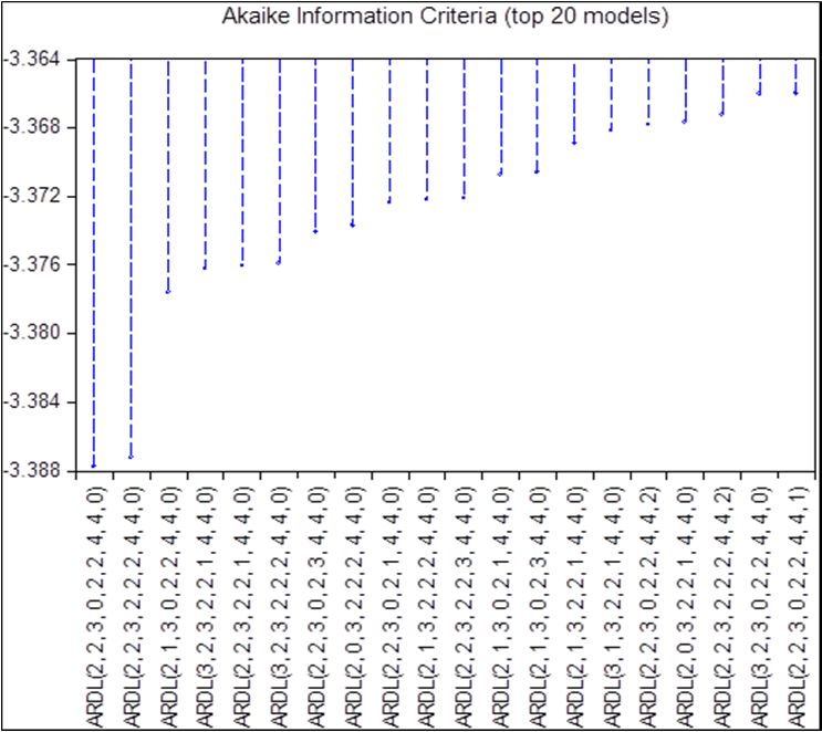
We will apply the criteria graph, which will indicate the suitable lags for the ARDL model and
the lowest value is preferred. Figure 6 shows the results of criteria graph for the ARDL model that
takes into account the number of new cases and new deaths in China, both for the BET stock index
return and for the Romanian Government bond (10Y).
According to the results, in total, 1,562,500 ARDL model specifications were considered for each
of the four cases given the information related to COVID-19 in China. The top 20 results are presented
in the criteria graph.
Further, Table 5 summarizes the selected lags for the model Romania and COVID-19 (China)
according to criteria graph out of Figure 6.
Table 5. Results of autoregressive distributed lags (ARDLs) for the model Romania and COVID-19
(China).
ARDL—The Number of New Cases in China due to COVID-19
BET_R ARDL(1, 0, 2, 1, 4, 1, 1, 2, 0)
RO_BOND ARDL(3, 2, 3, 2, 2, 1, 4, 4, 0)
ARDL—The Number of New Deaths in China due to COVID-19
BET_R ARDL(1, 0, 2, 1, 4, 1, 1, 2, 0)
RO_BOND ARDL(2, 2, 3, 0, 2, 2, 4, 4, 0)
Source: authors’ own calculations. Notes: for the definition of variables, please see Table 1.
Figure 7 shows the results of criteria graph for the ARDL model that takes into account the number
of new cases and new deaths in Italy, both for the BET stock index return and for the Romanian
Government bond (10Y). Likewise, in case of Italy, in total, 1,562,500 ARDL model specifications were
considered for each of the four cases.Int. J. Environ. Res. Public Health 2020, 17, 6729 14 of 35
Int. J. Environ. Res. Public Health 2020, 17, x 13 of 27
The number of new cases in China due to COVID-19
BET_R RO_BOND
The number of new deaths in China due to COVID-19
BET_R RO_BOND
Figure 6.
Figure 6. Optimal
Optimal lags
lags for
for the
the model
model Romania
Romania and
and COVID-19
COVID-19 (China).
(China). Source:
Source: authors’
authors’ own
own work.
work.
Notes: for the definition of variables, please see Table 1.
Notes: for the definition of variables, please see Table 1.
According
Table to the
6 exhibits results,
the in total,
selected 1,562,500
lags for the modelARDL modeland
Romania specifications were considered
COVID-19 (Italy) in line withfor each
criteria
of the four
graph cases
out of given
Figure 7. the information related to COVID-19 in China. The top 20 results are presented
in the criteria graph.
Further, Table
Table56.summarizes the lags
Results of ARDL selected lags
for the for the
model: model
Romania andRomania
COVID-19and COVID-19 (China)
(Italy).
according to criteria graph out of Figure 6.
ARDL—The number of new cases in Italy due to COVID-19
BET_R distributed lags (ARDLs)
Table 5. Results of autoregressive ARDL(1, 3, 2,
for the 4, 1, 0,
model 0, 0)
Romania and COVID-19 (China).
RO_BOND ARDL(1, 2, 2, 2, 2, 4, 4, 4)
ARDL—The Number of New Cases in China due to COVID-19
ARDL—The number of new deaths in Italy due to COVID-19
BET_R ARDL(1, 0, 2, 1, 4, 1, 1, 2, 0)
BET_R
RO_BOND ARDL(3,
ARDL(3, 2, 3,2,2,2,2,4,1,1,
4, 0, 4, 4)
4, 0)
RO_BOND
ARDL—The Number of New Deaths ARDL(2, 3, 1, due
in China 3, 3,to4,COVID-19
4, 2)
BET_R
Source: authors’ own ARDL(1,
calculations. Notes: for 0, 2, 1, 4,
the definition of1, 1, 2, 0) please see Table 1.
variables,
RO_BOND ARDL(2, 2, 3, 0, 2, 2, 4, 4, 0)
Source: authors’ own calculations. Notes: for the definition of variables, please see Table 1.
The results reported in Tables 7 and 8 provides the ARDL bound test for cointegration. If
the F-statistic is greater
Figure 7 shows than the
the results of upper
criteriabound,
graph forthenthethe variables
ARDL modelcomprised
that takesininto
theaccount
model are
the
cointegrated
number of new cases and new deaths in Italy, both for the BET stock index return and for(see
and a long-run relationship befall. With reference to new cases in China models the
Table 7), theGovernment
Romanian F-statistic for BET_R (18.06988)
bond (10Y). and RO_BOND
Likewise, in case of (4.523219)
Italy, inmodels is greater than
total, 1,562,500 ARDLthe model
upper
bound of bounds
specifications value
were at 5%, which
considered is suggesting
for each thatcases.
of the four long-run relationship occur between the variables.
The same result is achieved in the case of new deaths in China models, where the value of the F-StatisticInt. J. Environ. Res. Public Health 2020, 17, 6729 15 of 35
is greater than the upper bound critical value. Hence, the null hypothesis is rejected, meaning that
the variables in the model are cointegrated.
Int. J. Environ. Res. Public Health 2020, 17, x 14 of 27
The number of new cases in Italy due to COVID-19
BET_R RO_BOND
The number of new deaths in Italy due to COVID-19
BET_R RO_BOND
Figure 7. Optimal lags for the model Romania and COVID-19 (Italy). Source: authors’ own work.
Figure 7. Optimal lags for the model Romania and COVID-19 (Italy). Source: authors’ own work.
Notes: for the definition of variables, please see Table 1.
Notes: for the definition of variables, please see Table 1.
Table 6 exhibits
Regarding Italy, inthe selected
all four lags for
estimated ARDLthe models
model the Romania
existence andofCOVID-19
cointegration(Italy) in line with
is confirmed (see
criteria graph out of Figure 7.
Table 8) since the F-statistic is significantly higher than the critical values in I(0) and I(1). Consequently,
the examined variables are cointegrated and will move together in long-run.
Further, weTable 6. Resultsthe
will analyze of ARDL
resultslags for long-term
of the the model: Romania
linkages and COVID-19
between (Italy).
selected measures. Table 9
shows the outcomes regarding the long-run
ARDL—The numbercausal
of new connections among
cases in Italy due variables for the model Romania
to COVID-19
and COVID-19 (China)—newBET_R cases. The short-run ARDL(1, 3, 2, 4, 1,of
estimates 0, 0, 0)
ARDL approach are presented in
RO_BOND ARDL(1, 2, 2, 2, 2, 4, 4, 4)
Table S1. In the first model, the number of new infection cases from China have no effect on the BET
ARDL—The number of new deaths in Italy due to COVID-19
index return. However, a decrease BET_R
of crude oil price leads to a higher uncertainty, consistent with
ARDL(3, 2, 2, 4, 1, 0, 4, 4)
Salisu, Ebuh and Usman [23], suggesting
RO_BOND the necessity
ARDL(2, for3,policymakers
1, 3, 3, 4, 4, 2) to diminish fears in financial
markets. Source:
In addition,
authors’ theownexchange rate Notes:
calculations. negatively
for theinfluences
definition of stock market
variables, return
please in the1. long-run.
see Table
The Philadelphia Gold/Silver Index coefficient is positive and significant at the 5% level of significance.
Hence,Thetheresults reported
coefficient in Tables
of XAU_R 7 and that
indicates 8 provides the ARDL
an increase of one unitbound test for cointegration.
in Philadelphia Gold/Silver If the F-
Index
statistic
leads to is greater
over 0.2983than
unitstheincrease
upper bound,
in BETthen
indexthereturn
variables
in thecomprised
long-run.inThe theerror
model are cointegrated
correction term or
and a long-run
adjustment speedrelationship befall. With
provides evidence reference
regarding thetorate
new ofcases in Chinatomodels
convergence (see Table
equilibrium, being 7),highly
the F-
statistic for BET_R (18.06988) and RO_BOND (4.523219) models is greater than the upper bound of
statistically significant. The adjustment speed of −1.017783 shows that deviations from the long-term
bounds value
equilibrium inatBET
5%,index
whichreturn
is suggesting that long-run
are corrected relationship
the following day by occur between the
approximately variables.
101.7783 The
percent.
same result is achieved in the case of new deaths in China models, where the value of the F-Statistic
is greater than the upper bound critical value. Hence, the null hypothesis is rejected, meaning that
the variables in the model are cointegrated.Int. J. Environ. Res. Public Health 2020, 17, 6729 16 of 35
However, the short-run results show no impact of new infection cases of COVID-19 from China on
the BET index.
Table 7. The results of the ARDL bounds test for the model Romania and COVID-19 (China).
Null Hypothesis: No Long-Run Relationships Exist F-Statistic
The number of new cases in China due to COVID-19
BET_R 18.06988
RO_BOND 4.523219
The number of new deaths in China due to COVID-19
BET_R 18.40808
RO_BOND 5.358775
Critical Value Bounds
Significance I0 Bound I1 Bound
10% 1.95 3.06
5% 2.22 3.39
2.50% 2.48 3.7
1% 2.79 4.1
Source: authors’ own calculations. Notes: for the definition of variables, please see Table 1.
Table 8. The results of the ARDL bounds test for the model Romania and COVID-19 (Italy).
Null Hypothesis: No Long-Run Relationships Exist F-Statistic
The number of new cases in Italy due to COVID-19
BET_R 21.68051
RO_BOND 7.294209
The number of new deaths in Italy due to COVID-19
BET_R 18.94637
RO_BOND 5.32708
Critical Value Bounds
Significance I0 Bound I1 Bound
10% 2.03 3.13
5% 2.32 3.5
2.50% 2.6 3.84
1% 2.96 4.26
Source: authors’ own calculations. Notes: for the definition of variables, please see Table 1.
Regarding the second model from Table 9, similar to the first model, the new infection cases
from China does not influence Romania 10-year bond yield in the long-run. Unlike the previous
model, the RO_BOND is negatively affected by XAU_R and indicates that an increase of one unit in
Philadelphia Gold/Silver Index leads to over 0.3718 units decrease in RO_BOND return in the long-term.
Besides, in the long-run, the return of stock market index SSE 100 negatively influences Romania
10-year bond yield. The coefficient of the error correction term is highly statistically significant. Hence,
the Romanian 10-year bond will reach equilibrium with a speed of 185.3068 percent in next day. As
well, the short-run results strengthen the lack of impact regarding new infection cases of COVID-19
from China on RO_BOND.
Table 10 reveals the outcomes of the long-term connection amongst variables for the model
Romania and COVID-19 (China)—new deaths. The short-run results are shown in Table S2.Int. J. Environ. Res. Public Health 2020, 17, 6729 17 of 35
Table 9. ARDL long-run coefficients estimates for the model Romania and COVID-19 (China)—new cases.
ARDL—The Number of New Cases in China due to COVID-19
BET_R
Variables Coefficient Std. Error t-Statistic Prob. CointEq (−1)
SSE100_R 0.1616 0.1043 1.5489 0.1275 −1.017783(0)
EUR_CNY −1.3775 0.6322 −2.1790 0.0339
LSCO −0.0016 0.0009 −1.6941 0.0962
XAU_R 0.2983 0.0956 3.1188 0.0030
NATURAL_GAS −0.0022 0.0203 −0.1062 0.9159
CRUDE_OIL 0.0068 0.0020 3.3857 0.0014
WTI −0.0050 0.0015 −3.3472 0.0015
NC_CH 0.0000 0.0000 0.5168 0.6075
C −0.0110 0.0292 −0.3753 0.7090
RO_BOND
Variables Coefficient Std. Error t-Statistic Prob. CointEq (−1)
SSE100_R −0.73407 0.317581 −2.31143 0.0257 −1.853068 (0)
EUR_CNY −3.33276 1.262391 −2.64004 0.0115
LSCO 0.000428 0.001982 0.21588 0.8301
XAU_R −0.3718 0.140512 −2.64602 0.0113
NATURAL_GAS −0.0295 0.034367 −0.85833 0.3955
CRUDE_OIL −0.00673 0.00448 −1.50213 0.1404
WTI 0.006189 0.003557 1.74007 0.089
NC_CH −2E-06 0.000001 −1.22238 0.2282
C 0.061438 0.050715 1.21143 0.2323
Source: authors’ own calculations. Notes: for the definition of variables, please see Table 1.Int. J. Environ. Res. Public Health 2020, 17, 6729 18 of 35
Table 10. ARDL long-run coefficients estimates for the model Romania and COVID-19 (China)—new deaths.
ARDL—The number of new deaths in China due to COVID-19
BET_R
Variables Coefficient Std. Error t-Statistic Prob. CointEq (−1)
SSE100_R 0.161344 0.103218 1.563134 0.1241 −1.022253 (0)
EUR_CNY −1.40622 0.619485 −2.26998 0.0274
LSCO −0.00116 0.000982 −1.18237 0.2424
XAU_R 0.307503 0.094295 3.261086 0.002
NATURAL_GAS −0.01098 0.020597 −0.53307 0.5963
CRUDE_OIL 0.00646 0.002033 3.176981 0.0025
WTI −0.0049 0.00148 −3.31281 0.0017
ND_CH −3.5E-05 0.000041 −0.8348 0.4077
C 0.000795 0.029663 0.026797 0.9787
RO_BOND
Variables Coefficient Std. Error t-Statistic Prob. CointEq (−1)
SSE100_R −0.8325 0.375288 −2.21829 0.0316 −1.578551 (0)
EUR_CNY −2.29762 1.480246 −1.55219 0.1276
LSCO −0.00106 0.001518 −0.69786 0.4889
XAU_R −0.46095 0.162187 −2.84208 0.0067
NATURAL_GAS 0.007984 0.045281 0.176315 0.8608
CRUDE_OIL −0.00652 0.005282 −1.23372 0.2237
WTI 0.006963 0.004186 1.663637 0.1031
ND_CH 0.000009 0.000084 0.103675 0.9179
C 0.014044 0.066547 0.211036 0.8338
Source: authors’ own calculations. Notes: for the definition of variables, please see Table 1.Int. J. Environ. Res. Public Health 2020, 17, 6729 19 of 35
The empirical findings reveal that the impact is stronger in this case as compared to the model that
depends on the number of new cases in China due to COVID-19 (see Table 9). However, both models
shows that the number of new deaths in China due to COVID-19 has no influence on the BET index
return, respectively, on the Romania 10-year bond yield, neither in the short-term, nor in the long-term.
Therefore, both research hypotheses are rejected for Chinese COVID-19 figures, similar Topcu and
Gulal [86] which established that emerging European countries experienced the lowest influence of
the outbreak.
Tables 11 and 12 reveals the results of serial correlation and heteroscedasticity tests for the models
Romania and COVID-19 (China)—new cases and Romania and COVID-19 (China)—new deaths.
The results support that the models are free from autocorrelation and heteroscedasticity.
Table 11. Breusch–Godfrey serial correlation Lagrange multiplier (LM) test for the model Romania and
COVID-19 (China)—new cases and new deaths.
Breusch–Godfrey Serial Correlation LM Test
ARDL—The number of new cases in China due to COVID-19
BET_R
F-statistic 1.3637 Prob. F(2,50) 0.2651
Obs*R-squared 3.77603 Prob. Chi-Square(2) 0.1514
RO_BOND
F-statistic 1.551194 Prob. F(2,41) 0.2242
Obs*R-squared 5.135193 Prob. Chi-Square(2) 0.0767
ARDL—The number of new deaths in China due to COVID-19
BET_R
F-statistic 0.752052 Prob. F(2,50) 0.4767
Obs*R-squared 2.131861 Prob. Chi-Square(2) 0.3444
RO_BOND
F-statistic 2.743942 Prob. F(2,43) 0.0756
Obs*R-squared 8.262179 Prob. Chi-Square(2) 0.0161
Source: authors’ own calculations. Notes: The Obs*R-squared statistic is the Breusch-Godfrey LM test statistic. This
LM statistic is computed as the number of observations, times the (uncentered) R-squared from the test regression.
For the definition of variables, please see Table 1.
In the case of models that take into account the effects of new cases and new deaths in Italy,
unique relationships are identified between the selected variables, as opposed to the models that
explored the impact of coronavirus from China. Table 13 exhibits the outcomes of the long-term causal
associations between variables for the model Romania and COVID-19 (Italy)—new cases. The short-run
outcomes are exhibited in Table S3. In the long-run, the results of the first model show the lack of any
effect from the number of new cases of COVID-19 in Italy on BET index return. In contrast, the return
of Milan stock market index FTSE MIB has a positive long-term impact on the BET index return. As
well, the short-run results reveal no impact of new infection cases of COVID-19 from Italy on the BET
index return. In contrast to COVID-19 figures from China, in case of Italian new cases of coronavirus,
the first hypothesis is still rejected, but the second hypothesis is confirmed.
Moreover, in the second model, several statistically significant relationships are identified. There
is found a positive impact of the number of new cases in Italy on the Romania 10-year bond yield in
the long-term. In addition, a natural gas futures contract has a positive effect on RO_BOND, while
the WTI Oil and Philadelphia Gold/Silver Index has a negative impact in the long-run. Another
outstanding outcome is that new infection cases of COVID-19 from Italy negatively influence RO_BOND
in the short-run, consistent with Sène, Mbengue and Allaya [36]. Therefore, the related uncertainty
triggered by the health emergency may determine investors to get rid of their securities.
Table 14 exposes the findings towards long-run linkages between variables for models related
to Romania and COVID-19 (Italy)—new deaths. The results of short-run estimates are presented in
Table S4.Int. J. Environ. Res. Public Health 2020, 17, 6729 20 of 35
Table 12. Heteroscedasticity test: Breusch–Pagan–Godfrey for the model Romania and COVID-19
(China)—new cases and new deaths.
Heteroscedasticity Test: Breusch–Pagan–Godfrey
ARDL—The number of new cases in China due to COVID-19
BET_R
F-statistic 1.998167 Prob. F(20,52) 0.0237
Obs*R-squared 31.72268 Prob. Chi-Square(20) 0.0463
RO_BOND
F-statistic 1.088975 Prob. F(29,43) 0.3929
Obs*R-squared 30.91112 Prob. Chi-Square(29) 0.3696
ARDL—The number of new deaths in China due to COVID-19
BET_R
F-statistic 1.228936 Prob. F(20,52) 0.2699
Obs*R-squared 23.43009 Prob. Chi-Square(20) 0.2682
RO_BOND
F-statistic 1.062309 Prob. F(27,45) 0.4193
Obs*R-squared 28.41672 Prob. Chi-Square(27) 0.3897
Source: authors’ own calculations. Notes: The Obs*R-squared statistic for the Breusch-Pagan-Godfrey test is
computed by multiplying the sample size by the coefficient of determination of the regression of squared residuals
from the original regression. For the definition of variables, please see Table 1.
The first model out of Table 14 exhibits that the number of new deaths from Italy have no effect
on the BET index return in the long-run. The Philadelphia Gold/Silver Index coefficient is positive
and significant at the 5% level of significance. Hence, the coefficient value of XAU_R indicates
that an increase of one unit in Philadelphia Gold/Silver Index leads to over 0.1574 units increase in
BET index return in the long-term. However, the short-run results show a negative impact of new
deaths cases of COVID-19 from Italy on the BET index return, in line with Okorie and Lin [58] which
underlined a transitory contagion effect in the stock markets due to novel coronavirus. In addition,
Erdem [55] claimed that the index returns decline and volatilities rise due to corona crisis. Hence,
the first hypothesis is confirmed.
The second model shows a negative effect of the new deaths’ cases from Italy on the Romania
10-year bond yield in the long-run. In addition, the Philadelphia Gold/Silver Index and the OK crude oil
future contract negatively influence RO_BOND in the long-term. Besides, in the long-run, the returns
of the stock market index FTSE MIB has no impact on the 10-year Romanian bond. Nevertheless,
in the short-run, results show a negative impact of new deaths cases of COVID-19 from Italy on
the RO_BOND. Therefore, the second hypothesis is established.
Tables 15 and 16 exhibit the outcomes of Breusch—Godfrey Serial correlation LM test and
Breusch–Pagan–Godfrey heteroscedasticity test for the models Romania and COVID-19 (Italy)—new
cases and Romania and COVID-19 (Italy)—new deaths. Hence, the models are not threatened by
autocorrelation and heteroscedasticity.
4.3. Causality Investigation
With the purpose of exploring the causality between included variables, the Granger causality
test is employed. In order to be able to apply the Granger causality test, the data series must be
stationary and therefore they were turned it into stationary series. Table 17 displays the results of
Granger causality test for the stock market returns and COVID-19 measures. There were identified
some bidirectional causal relations between BET_R and FTMIB_R (1st lag), as well as among BET_R and
IBEX35_R (1st lag). Besides, some unidirectional causal relations arise from FTSE_R (1st lag), DJIA_R
(1st lag and 3rd lag), SSE100_R (1st lag, 2nd lag, and 3rd lag), and XAU_R (1st lag, 2nd lag, and 3rd lag)
to BET_R. Nevertheless, no relationship was found between BET_R and the COVID-19 variables.You can also read