Aggregate and Firm-Level Stock Returns During Pandemics, in Real Time
←
→
Page content transcription
If your browser does not render page correctly, please read the page content below
Aggregate and Firm-Level Stock Returns
                      During Pandemics, in Real Time∗
       Laura Alfaro†          Anusha Chari‡          Andrew Greenland§             Peter K. Schott¶

                                               May 10, 2020

                                     Preliminary and Incomplete
                                         Comments Welcome!
                                     Most recent version is here
                                       First Draft: March 25, 2020

                                                  Abstract

      We show that unexpected changes in the trajectory of COVID-19 infections predict US stock
      returns, in real time. Parameter estimates indicate that an unanticipated doubling (halving) of
      projected infections forecasts next-day decreases (increases) in aggregate US market value of 4
      to 11 percent, indicating that equity markets may begin to rebound even as infections continue
      to rise, if the trajectory of the disease becomes less severe than initially anticipated. Using the
      same variation in unanticipated projected cases, we find that COVID-19-related losses in market
      value at the firm level rise with capital intensity and leverage, and are deeper in industries
      more conducive to disease transmission. These relationships provide important insight into
      current record job losses. Measuring US states’ drops in market value as the employment
      weighted average declines of the industries they produce, we find that states with milder drops
      in market value exhibit larger initial jobless claims per worker. This initially counter-intuitive
      result suggests that investors value the relative ease with which labor versus capital costs can
      be shed as revenues decline.

  ∗
     This paper is preliminary and incomplete. We thank Nick Barberis, Lorenzo Caliendo, Patrick Conway, Teresa
Fort, Mihai Ion, Ed Kaplan, John Lopresti, and seminar participants from Duke and UNC TEAM working group as
well as the CEPR Covid-Economics virtual seminar series for comments and suggestions. We thank Alex Schott and
Mengru Wang for excellent research assistance.
   †
     Harvard Business School & NBER (lalfaro@hbs.edu).
   ‡
     UNC Chapel Hill & NBER (achari@unc.edu).
   §
     Martha and Spencer Love School of Business, Elon University (agreenland@elon.edu).
  ¶
     Yale School of Management & NBER (peter.schott@yale.edu).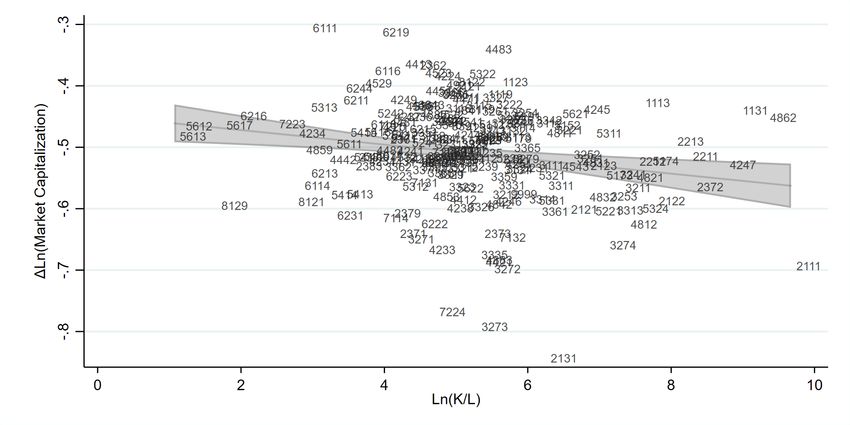
1       Introduction
The tension between Wall-Street and Main Street during the COVID-19 pandemic is palpable. In
the early weeks of the outbreak, US equity markets dropped 35 percent. Then, even as reported
infections continued to rise, and jobless claims surged, the stock market rallied. In this paper we
investigate how information about the expected impact of pandemics is incorporated into aggregate
and firm-level stock returns, day by day. Our results provide a rationale for the seemingly divergent
paths of the US equity and labor markets.
    We begin by showing that unanticipated changes in predicted infections based on daily re-
estimation of simple epidemiological models of infectious disease forecast next-day stock returns.
While our focus is on the current COVID-19 crisis in the United States, we find a similar pattern
during the 2003 SARS outbreak in Hong Kong. In each case, larger changes in model predictions
are associated with greater changes in market returns, in both directions.1
    Estimates for the United States thus far indicate that a doubling (halving) of predicted COVID-
19 infections is associated with a decline (increase) of 4 to 10 percent in the Wilshire 5000 index.
These findings are consistent with investors using such models to update their beliefs about the
economic consequences of the outbreak, in real time. They suggest that equity markets may par-
tially recover, and become less responsive to new cases, if the trajectory of the pandemic becomes
less severe than initially anticipated, and more certain. As a consequence, they provide an expla-
nation for the confusion expressed in recent newspaper articles about the recovery of the US stock
market in April: this recovery coincides with a flattening out of unanticipated changes in predicted
infections.2
    We use the same variation in predicted infections to examine exposure to COVID-19 at the
industry and firm levels. We show that industries more conducive to virus transmission – Accom-
modations, Entertainment and Transportation – exhibit the greatest exposure to the pandemic, and
the largest declines in market value. Education, Professional Services and Finance, by contrast,
are less sensitive, likely due to a greater ability to continue operations online. At the firm level,
we find that COVID-19-driven changes in market value are almost universally negative, that they
vary widely both within and across sectors, and that more capital-intensive, more debt-laden, and
less profitable firms exhibit larger declines.3
    We interpret these results as signaling investors’ expectation that firms which are more able to
shed costs during the pandemic will have smaller losses, and thus relatively higher returns.4 As
debt is non-dischargable, and nearly all property, plant and equipment is sunk in a macroeconomic
downturn of COVID-19’s magnitude, debt-laden and capital-intensive firms are less likely to be
able to reduce costs as revenues decline. Labor-intensive firms’ relatively high returns, by contrast,
reflect the relative ease with which workers (versus capital) can be furloughed or dismissed as the
economy contracts.
    Further evidence in favor of this mechanism comes from an analysis of jobless claims across
regions. We construct county- and state-level measures of equity market exposure to COVID-19
as the employment weighted average COVID-19-related change in market value across the 4-digit
NAICS sectors they produce (Bartik, 1991). We interpret this exposure as the translation of
    1
     We are expanding the set of countries we analyze for the COVID-19 outbreak, and are investigating other
pandemics, e.g., the 2009 H1N1 outbreak. These results will appear in a future draft.
   2
     See, for example, “Prescient or Pollyannaish? Explaining the Market’s Rally” in the April 18, 2020 edition of
the Wall Street Journal.
   3
     Ramelli and Wagner (2020) and Albuquerque et al. (2020) also document the negative association between market
returns and debt during COVID-19.
   4
     Baker et al. (2020) show that a near ubiquitous decline in US consumption during late March and April.

                                                        1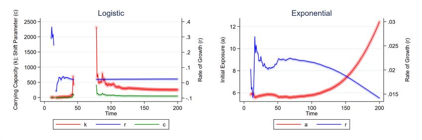
unanticipated news about the pandemic from firms to states.
    Using a difference-in-differences specification, we demonstrate that states with milder average
declines in market value exhibit greater growth in initial jobless claims per worker. This initially
counter-intuitive finding is consistent with the negative relationship between firm capital intensity,
leverage and market returns noted above. Highly leveraged, more capital-intensive firms likely
have less flexibility with respect to reducing costs during the pandemic than labor-intensive firms,
as property, plant and equipment cannot be shed as easily as labor during the extreme economic
contraction. Thus, states with a greater proportion of labor-intensive firms exhibit less decline in
average market value, but greater proportional shedding of workers. To the best of our knowledge,
we are the first to use equity prices to quantify the spatial incidence of a macroeconomic shock,
and among the first to examine regional variation in COVID-19-driven initial jobless claims.5
    Our analysis contributes to several literatures. First, we add to the very large body of research
on asset pricing that examines the predictability of stock returns (e.g. Campbell and Shiller (1988),
Fama and French (1988)) and, more specifically, to recent research examining the financial market
consequences of COVID-19, lead by Ramelli and Wagner (2020). One set of papers in this bur-
geoning literature associates Ball and Brown (1968) and Fama et al. (1969) style abnormal returns
during the pandemic to various firm characteristics.6 A second group seeks to identify channels of
firm exposure via ex-ante observable firm or aggregate characteristics.7
    While similar in spirit, our analysis differs from these two sets of papers both methodologically
and quantitatively, as we relate returns to exogenous changes in investors’ information about the
trajectory of the pandemic, as it unfolds. Specifically, we model cumulative infections during an
outbreak as following either an exponential or a logistic curve. We re-estimate the parameters of
these models each day of the outbreak using information on reported cases up to that day. More
precisely, we predict infections for trading day t using the cumulative counts as of the end of days
t − 1 and t − 2. The differences in these forecasts represent unanticipated changes in the trajectory
of the disease due to newly available information, and we examine how they covary with both
aggregate and firm-level market returns on day t.8
    As a robustness exercise, we demonstrate that the information in daily predicted infections dom-
inates the most recent change in reported infections in forecasting stock returns. This dominance
is understandable, in that the anticipated portion of the most recent reported case growth has
already been priced into equities. It is precisely the unanticipated portion of this growth, however,
that updates investors’ expectations regarding the eventual number of infections, the speed with
which that number may be reached, and the associated economic consequences. Indeed, jumps in
estimated share of the population that ultimately will be infected, or the growth rate of infections,
signal larger potential declines in demand for goods and services, especially those which might
facilitate transmission. Changes in these parameters may also indicate greater shocks to labor
supply due to sickness or implementation of social distancing policies, further hampering aggregate
demand (Guerrieri et al., 2020). In a related robustness exercise, we show that our results for the
United States are robust to the inclusion of coarse controls for changes in federal and local policy.
    Relative to existing research on the financial implications of COVID-19, our approach offers
   5
     Closely related is Greenland et al. (2019) who use equity market derived measures to explore the employment
consequences of the United States’ granting Permanent Normal Trade Relations to China in 2001.
   6
     See, for example, Ramelli and Wagner (2020); Albuquerque et al. (2020); Ru et al. (2020).
   7
     See, for example, Baker et al. (2020); Fahlenbrach et al. (2020); Ding et al. (2020); ?
   8
     We emphasize that we are not epidemiologists and are not outlining a method to characterize the true path of
pandemics. Nor are we, like Piguillem and Shi (2020) and Berger et al. (2020), trying to infer the efficacy of various
intervention strategies. Such efforts, while of immense value, require data which may not be available until after the
outbreak is substantially underway. Rather, we view real-time changes in the predicted severity of an outbreak as
potentially useful summary statistics of its ultimate economic consequences.

                                                          2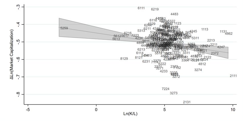
three benefits. First, it does not require us to calculate firms’ expected normal rate of return
with the aid of an asset pricing model – e.g. the CAPM (Sharpe, 1964a) – estimated during a
period before COVID-19. In fact, estimates of abnormal returns utilizing such models may be mis-
specified if their true values can be inferred only in the presence of disaster risk (Bai et al., 2019).
Second, our approach yields firm-level measures of exposure without identifying their channels
ex-ante, and without attributing all aggregate movement in returns to COVID-19. Given the
unprecedented nature of this event, this benefit is sizeable. Finally, by exploiting changes in the
forecasted trajectory of the pandemic between market close on day t − 1 and opening on day t,
our approach exploits only new information about the trajectory of the pandemic and therefore
can rationalize both market upswings and downturns. Our findings suggest that investors, facing
substantial uncertainty about the true economic fallout of this realized tail risk (Knight, 1921;
Keynes, 1937), may be availing themselves of changes in daily case forecasts as a summary statistic
for the ultimate scale and economic fallout of the epidemic.
    Our paper also contributes to the very large literature in public health which attempts to explain
the trajectory of infections during a pandemic.9 In contrast to that research, we link changes in
the estimated parameters and predictions of these models in real time to economic outcomes. To
reiterate, we do not claim that the evolution of a pandemic must follow a purely exponential or
logistic growth path. Rather, we explore whether the predictions of these models are informative
of economic conditions, as manifest in their correlation with the market.10
    Finally, this paper relates to a rapidly emerging literature studying the aggregate economic
consequences of COVID-19, and a more established literature investigating earlier pandemics. Barro
et al. (2020) draws parallels between COVID-19 and the “Spanish Flu” to forecast changes in
economic activity, while Baker et al. (2020) documents that the COVID-19 pandemic is the first
infectious disease outbreak whose mention in the press is associated with a large daily market
movement. Our analysis complements the equity market studies of Gormsen and Koijen (2020) and
Baker et al. (2020), who link COVID-19 financial market reactions to future GDP growth. It also
relates to the labor market studies of Cajner et al. (2020) and Coibion et al. (2020), which analyze
employment trends during COVID-19, and the examinations of labor market interactions during
COVID-19 more directly in Humphries et al. (2020) and Bartik et al. (2020). In contrast to these
efforts, we exploit exogenous variation in investors’ expectations about the pandemic’s trajectory
to identify aggregate and firm-level exposure, which we then link to labor market outcomes.
    This paper proceeds as follows. Section 2 provides a brief description of infectious disease
models and how investors might link the predictions of these models and to asset prices. Sections
3 and 4 apply our framework to COVID-19 and SARS. Section 5 concludes.

2       Modeling
In this section we outline how infectious disease outbreaks can be modeled in real time, and how
investors might make use of the model’s estimated parameters.

2.1     Simple Models of Infectious Diseases
Exponential and logistic growth models are frequently used in biology and epidemiology to model
infection and mortality. An exponential model,
    9
     Early contributions to this literature include Ross (1911), Kermack and McKendrick (1927), Kermack and McK-
endrick (1937) and Richards (1959).
  10
     For an interesting discussion on the complexities associated with modeling an outbreak in real time, see https:
//fivethirtyeight.com/features/why-its-so-freaking-hard-to-make-a-good-covid-19-model/.

                                                         3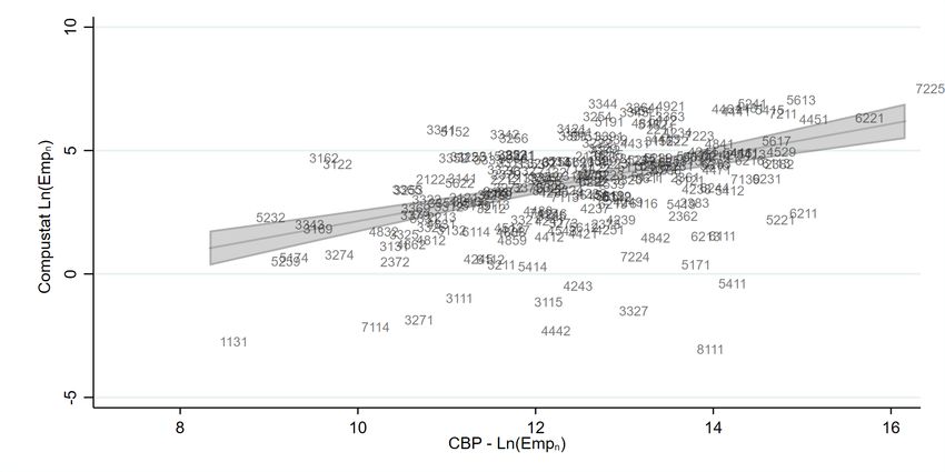
Ct = ae(rt)                                               (1)
predicts the cumulative number of cases on day t, Ct , as a function of the growth rate of infections
in that country, r, the initial number of infected persons a, and time. In an exponential model, the
number of infections per day continues to climb indefinitely. While clearly unrealistic ex-post, the
exponential growth model is consistent with early stage pandemic growth rates.
     In a logistic model (Richards, 1959), by contrast, the growth in infections grows exponentially
initially, but then declines as the stock of infections approaches the population’s “carrying-capacity,”
i.e., the cumulative number of people that ultimately will be infected. Carrying capacity is generally
less than the full population. The cumulative number of infections on day t is given by

                                                            k
                                                Ct =               ,                                          (2)
                                                       1 + ce(−rt)
where k is the carrying, c is a shift parameter (characterizing the number of initially infected
persons) and r is the growth rate. Figure 1 provides an example of logistic infections for three
different growth rates (2.5, 5 and and 7.5 percent) assuming k = 250 and c = 50. For each growth
rate, we plot both the number of new cases each day (right axis) and the cumulative number of
cases up to each day (left axis). As indicated in the figure, higher growth rates both shorten the
time required to reach carrying capacity and increase the peak number of infections.

                Figure 1: New and Cumulative New Cases Under the Logistic Model

                            Source: Authors’ calculations. Figure compares new and cumu-
                            lative infections from days 1 to 200 assuming a logistic model
                            with k = 250 and c = 50 and noted growth rates (r).

    Given data on the actual evolution of infections, the two parameters in equation 1 and the
three parameters in equation 2 can be updated each day using the sequence of infections up to that
date. We estimate these sequences using STATA’s nonlinear least squares command (nl).11 This
command requires a vector of starting values, one for each parameter to be estimated.
    We encounter two problems during our estimation of logistic functions in our applications below.
First, estimates for each day t are sensitive to the choice of starting values for that day, particularly
in the initial days of the pandemic. This feature of the estimation is not surprising: when the
number of cases is relatively small, a wide range of logistic curves may be consistent with the data,
and the objective function across them may be relatively flat.
  11
     We are exploring other estimation procedures for use in a future draft, including use of SIR and SEIR models,
e.g., Li et al. (2020) and Atkeson (2020).

                                                          4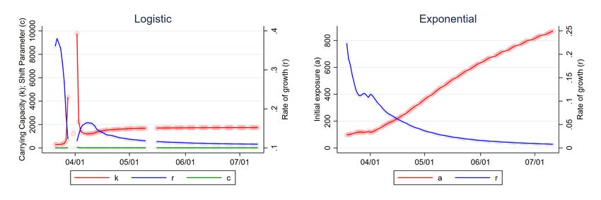
To increase the likelihood that our parameter estimates represent the global solution, we estimate
500 epidemiological models for each day, 250 for the logistic case, and 250 for the exponential case.
In each iteration we use a different vector of starting values. For each day t, our first starting values
are the estimated coefficients from the prior day, if available.12 In the case of the logistic model,
we then conduct a grid search defined by all triples {r, c, k} such that

                                          r ∈ {0.01, 0.21, 0.41, 0.61, 0.81}
                                          t−1 , 2 ∗ cd
                                    c ∈ {cd          t−1 , 4 ∗ cd
                                                                t−1 , . . . , 10 ∗ cd
                                                                                    t−1 }

                                         t−1 , 2 ∗ kd
                                   k ∈ {kd          t−1 , 3 ∗ kd
                                                               t−1 , . . . , 10 ∗ kd
                                                                                   t−1

where hats over variables indicate prior estimates, and superscripts indicate the day on which they
are estimated. If more than one of these initial starting values produces estimates, we choose the
parameters from the model with the highest adjusted R2 . We estimate the exponential model
similarly.
    The second, more interesting, problem that we encounter during estimation of the logistic
outbreak curves is that STATA’s nl routine may fail to converge. This failure generally occurs in
the transition from relatively slow initial growth to subsequent, more obviously exponential growth
as the pandemic proceeds. During this phase of the outbreak, the growth in the number of new
cases each day is too large to fit a logistic function, i.e., the drop in the growth of new cases
necessary to estimate a carrying capacity has not yet occurred.13
    In our application below, we re-estimate both exponential and logistic parameters each day of
an outbreak. To fix ideas, we simulate a 200-day cumulative logistic disease outbreak by generating
a sequence of Ct = 1+cek(−rt) + |t | for t ∈ (1 : 200), assuming k = 250, r = .025, c = 50 and |t |
is the absolute value of a draw from a standard normal distribution. For each day t, we estimate
logistic and exponential parameters using the sequence of simulated infections up to that day.
    Figure 2 displays the results. Both sets of parameter estimates are volatile in the early stage
of the outbreak. Logistic parameters are not available from days 47 through 78 due to lack on
convergence, but settle down shortly thereafter, as the data increasingly conform to underlying
logistic path. Exponential parameters are available for each day, but do not settle down as time
goes on. The intuition for the unending increase in abt and decline in rbt is as follows: because the
simulated data are logistic, the only way to reconcile them with an exponential function is to have
the estimate of initial exposure (abt ) rise as the estimate of the growth rate, rbt , drops.
 12
      If the prior day did not converge, we use the most recent prior day for which we have estimates.
 13
      In a future draft we will consider an estimation strategy that nests these functions.

                                                             5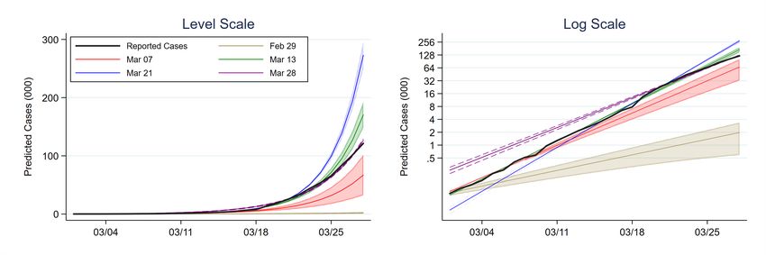
Figure 2: Parameter Estimates Using Simulated Logistic Pandemic

       Source: authors’ calculations. The left panel plots the sequence of logistic parameters, kbt , cbt and rbt , estimated
       using the information up to each day t on simulated data (see text). Right panel of Figure plots the analogous
       sequence of exponential parameters, abt and rbt , using the same data. Missing estimates indicate lack of
       convergence (see text). Circles represent estimates. Solid lines connect estimates.

    Figure 3 compares predicted cumulative cases for each model for each day t using the parameter
                                                        [t−1
estimates from day t − 1. We denote these predictions C      , where the superscript t − 1 refers to
                                                                             t
the timing of the information used to make the prediction, and the subscript refers to the day
being predicted. As illustrated in the figure, predictions for the two models line up reasonably
well during the initial phase of the pandemic. Their 95 percent confidence intervals (not shown)
cease overlapping on t = 104. After this point, the exponential model continues to project an
ever-increasing number of infections, while the logistic model’s predictions head towards the “true”
carrying capacity of 250.

                                                                         [ t−1
                         Figure 3: Simulated Pandemic Daily Predictions (C t   )

                    Source: authors’ calculations. Figure compares simulated “actual” cumulative in-
                                                      \ t−1
                    fections to predicted infections (C   t ) under the logistic and exponential models.
                    The prediction for each day t is based on the information available up to day t − 1.
                    The two vertical lines in the figure note when the 95 percent confidence intervals
                    of the two models’ predictions (not shown) initially diverge, and when the logistic
                    model’s estimates first indicate that its inflection point has passed.

                                                                 6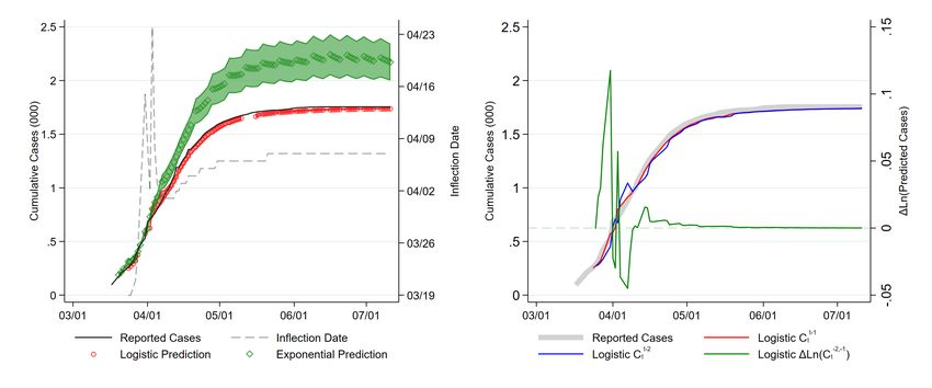
2.2      Modeling Economic Impact
                                                                     [ t−1
Predicted cumulative cases for day t based on day t − 1 information, C t   , can be compared to the
                                                [ t−2
day t forecast made with day t − 2 information, C . The log difference in these predictions,
                                                              t

                                      −2,−1
                                 ∆ln C\
                                      t
                                                         [
                                                    = ln C t−1
                                                           t
                                                                           [t−2
                                                                      − ln Ct     ,                               (3)

captures unexpected changes in severity of the outbreak between these two days.14 This potentially
noisy “news” may be an important input into investors’ assessment of the economic impact of
a pandemic. For example, jumps in estimated growth rates or carrying capacites signal larger
potential declines in demand, reducing firm revenue. Increases in these parameters may also presage
more substantial declines in labor supply, or the implementation of social distancing policies that
further reduce demand (Guerrieri et al., 2020).

3        Application to COVID-19
In this section we provide real-time estimates of the outbreak parameters and infection predictions
for COVID-19 in the United States. We then examine the relationship between changes in these
predictions and both aggregate and firm-level returns in the United States.

3.1      Epidemiological Model Paremeters
Data on the cumulative number of COVID-19 cases in the United States as of each day are from
the Johns Hopkins Coronavirus Resource Center.15 The first COVID-19 case appeared in China
in November of 2019, while the first cases in the United States and Italy appeared on January 20,
2020. Our analysis begins on January 22, 2020, the first day that the World Health Organization
began issuing situation reports detailing new case emergence internationally. Appendix Figure A.1
displays the cumulative reported infections in the United States from January 22 through April 10,
2020.
     We estimate logistic and exponential parameters (equations 1 and 2) for the United States by
day as discussed in Section 2.1. The daily parameter estimates for the logistic estimation, kbt , cbt
and rbt are displayed the left panel of Figure 4, while those for the exponential model, abt and rbt , are
reported in the right panel. Gaps in the time series in either figure represent lack of convergence.
     Logistic parameter estimates for the United States fail to converge after February 23, when
the number of cases jumps abruptly from 15 to 51. That no parameter estimates are available
after this date suggests that growth in new cases observed thus far is inconsistent with a leveling
off, or carrying capacity, at least according to our estimation method. The exponential model, by
contrast, converges for all days. As a result, we focus on the exponential model for the remainder
of our analysis.
     As the sharp changes in US exponential model parameters suggest, predicted cumulative infec-
tions vary substantially depending upon the day in which the underlying parameters are estimated.
    14
    Timing is as follows: the number of infections on day t − 1 is observed after the market closes on that day but
                                                                                                               [ t−1
before the market opens on day t. This day t − 1 information is used to predict the number of cases for day t, C t   ,
                       [t−2
which is compared to C .t
    15
    These data can be downloaded from https://github.com/CSSEGISandData/COVID-19 and visualized at https:
//coronavirus.jhu.edu/map.html.

                                                          7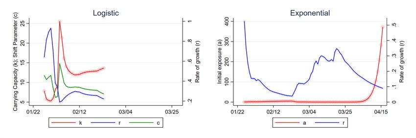
Figure 4: Parameter Estimates for COVID-19

             Source: Johns Hopkins Coronavirus Resource Center and authors’ calculations. The left panel
             plots the sequence of logistic parameters, kcit , cc
                                                                it and rc
                                                                        it , estimated using the cumulative in-
             fections in the US up to each day t. Right panel plots the analogous sequence of exponential
             parameters, acit and rcit , using the same data. Missing estimates indicate lack of convergence
             (see text). Circles represent estimates. Solid lines connect estimates. Data currently extend to
             Friday March 27, 2020.

Figure 5 highlights this variability by comparing predicted cumulative infections based on the in-
formation available as of February 29 and March 7, 13, 21 and 28. The left panel displays these
projections in levels, while the right panel uses a log scale. The five colored lines in the figure trace
out each set of predictions. Dashed lines highlight 95 percent confidence intervals around these
predictions. Finally, the confidence intervals are shaded for all days following the day upon which
the prediction is based. To promote readability, we restrict the figure to the period after February
29. The black, solid line in the figure represents actual reported cases.

      Figure 5: Predicted Cumulative Cases Using Different Days’ Estimates (COVID-19)

             Source: Johns Hopkins Coronavirus Resource Center and authors’ calculations. Figure displays
             predicted cases for the United States from March 18 onwards using the cumulative reported
             cases as of five dates: February 29, March 7, March 13, March 21 and March 28. Dashed lines
             represent 95 percent confidence intervals. Confidence intervals are shaded for all days after the
             information upon which the predictions are based.

    Predicted cumulative infections based on information as of February 29 are strikingly lower
than predictions based on information as of March 21 due to the jump in reported cases between
those days. Indeed, according to the parameter estimates from March 21, US cases would number
close to 300 thousand by the end of March. Equally striking is the downward shift in predicted
cumulative cases that occurs between March 21 and March 28. It is precisely these kinds of changes
in predicted cumulative cases that our analysis seeks to exploit.
                                                                          [ t−1      [t−2
    Figure 6 uses the exponential parameter estimates in Figure 4 to plot C     and C     , i.e., the
                                                                                                 t                t
predicted number of cases on day t using the information up to day t − 1 and day t − 2. Magnitudes
for these cumulative cases are reported on the left axis.

                                                             8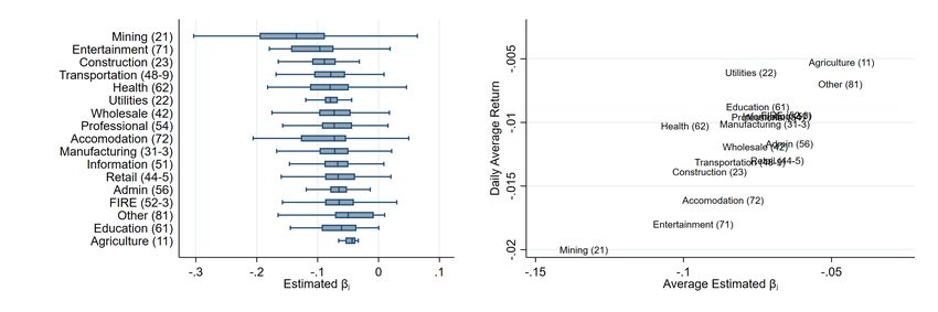
−2,−1
                                                  [
            Figure 6: Daily Logistic Predictions (C t−1
                                                    t   and ∆ln(C\
                                                                 t     )) for COVID-19

                          Source: Johns Hopkins Coronavirus Resource Center and authors’ cal-
                          culations. Left axis reports the predicted cumulative cases for day t
                                                             \ t−1                  \ t−2
                          using information as of day t − 1, C  t  , and day t − 2, Ct    , under
                          the exponential model. Right axis reports the log change in these two
                          predictions, ∆ln(Ct−2,−1 ). Data currently extend to Friday April 10,
                                            \
                          2020.

                                             −2,−1
    The right axis in Figure 6 reports ∆(C\  t     ), the log difference in these two predictions. Intu-
         [ t−1     [ t−2
itively, C t   and C t   for the most part track each other closely. The former rises above the latter
on days when reported cases jump, while the reverse happens when new cases are relatively flat.
                                         [ t−2
The scalloped pattern of exhibited by C        after March 25 captures the relatively smooth decline
                                                 t
in ac
    it and rise in r
                   c it (displayed in Figure 4) required for the exponential function to capture the
increasingly logistic data.

3.2    Aggregate US Returns During COVID-19
We examine the link between changes in model predictions and aggregate US stock via the Wilshire
5000 index.16 We choose this index for its breadth, but note that results are qualitatively similar
for other US market indexes.
    Figure 7 plots the daily log change in the Wilshire 5000 index against unanticipated increases
                 −2,−1
in cases, ∆ln(C\   t   ). Their negative relationship indicates that returns are higher when the
difference in predictions is lower, and vice versa. In particular, the approximate 20 percent decline
in predicted cases that occurs on March 24 coincides with a greater than 9 percent growth in the
market index.
    We compare aggregate equity returns on day t to the difference in forecasts for that day formally
using an OLS regression,

                                                         \−2,−1
                        ∆ln (Indext ) = α + γ1 ∗ ∆ln Ct            + γ2 Xt + t .                 (4)

where ∆ln (Indext ) is the daily log change in either opening-to-opening or closing-to-closing prices
in the Wilshire 5000, and Xt represents a vector of controls, e.g., changes in policy.17 The estimation
period consists of 52 trading days from January 22 to April 10.18 The unit of observation is one
  16
     Data for the Wilshire 5000 are downloaded from Yahoo Finance.
  17
     We are currently exploring more flexible specifications, e.g., those which might capture the switch between
exponential and logistic models, as well as those which reveal any over- or undershooting of reactions.
  18
     The actual number of trading days between these two dates is 50. We lose 3 days due to lack of estimates in the

                                                            9
−2,−1
Figure 7: Change in Predicted COVID-19 Cases (∆C\
t ) vs Aggregate Market Returns
Source: Johns Hopkins Coronavirus Resource Center, Yahoo Finance and authors’ calculations.
Figure displays the daily log change in the Wilshire 5000 index against the log change in pre-
dicted cases under the exponential model for day t based on day t − 1 and day t − 2 information.
Sample period is January 22 to April 10, 2020.
day.
−1,−2
Table 1: Changes in Predicted COVID-19 Cases (∆C\
t ) vs Market Open Returns
(1) (2) (3) (4) (5) (6)
∆Ln(Open) ∆Ln(Open) ∆Ln(Open) ∆Ln(Open) ∆Ln(Open) ∆Ln(Open)
−2,−1 )
∆Ln(C\ -0.040∗∗∗ -0.049∗∗ -0.061∗∗ -0.063∗∗ -0.085∗∗ -0.055∗∗
(0.013) (0.024) (0.024) (0.025) (0.033) (0.025)
∆Ln(C −2,−1 ) 0.019 0.026 0.028 0.006
(0.028) (0.026) (0.026) (0.033)
I(∆SIndex) -0.014
(0.014)
∆Ln(SIndex) -0.055
(0.061)
Fiscal Stimulus 0.017
(0.013)
Constant -0.007∗ -0.005 -0.008∗∗ -0.007∗ -0.006 -0.008∗
(0.004) (0.004) (0.004) (0.004) (0.004) (0.004)
Observations 47 47 47 47 43 47
R2 0.084 0.069 0.078 0.121 0.144 0.118
Daily Adjustment N Y Y Y Y Y
Source: Johns Hopkins Coronavirus Resource Center and authors’ calculations. ∆Ln(Opent ) and
∆Ln(Closet ) are the daily log changes in the opening (i.e., day t − 1 to day t open) and closing values
−2,−1
of the Wilshire 5000. ∆ln(C\ ) is the change in predicted cases. ∆ln(C −2,−1 ) is the change in
t t
actual observed cases between days t − 2 and t − 1. ∆ln(Ct−1,0 ) is the change in actual observed cases
between days t − 1 and t. Robust standard errors in parenthesis. Columns 2-6 divide all variables by
the number of days since the last observation (i.e., over weekends). Sample period is January 22 to
April 10, 2020.
initial days of the outbreak.
10−2,−1
Table 2: Change in Predicted COVID-19 Cases (∆C\
t ) vs Market Close Returns
(1) (2) (3) (4) (5) (6)
∆Ln(Close) ∆Ln(Close) ∆Ln(Close) ∆Ln(Close) ∆Ln(Close) ∆Ln(Close)
−2,−1 )
∆Ln(C\ -0.067∗∗ -0.080∗∗ -0.089∗∗∗ -0.093∗∗∗ -0.146∗∗∗ -0.089∗∗∗
(0.030) (0.030) (0.031) (0.034) (0.041) (0.032)
∆Ln(C −1,−0 ) 0.033 0.055 0.065∗ 0.034
(0.031) (0.037) (0.035) (0.032)
I(∆SIndex) -0.021
(0.018)
∆Ln(SIndex) -0.091
(0.076)
Fiscal Stimulus -0.005
(0.018)
Constant -0.009 -0.005 -0.010∗∗ -0.010∗∗ -0.010∗∗ -0.010∗∗
(0.006) (0.005) (0.004) (0.004) (0.004) (0.004)
Observations 47 47 47 47 43 47
R2 0.092 0.086 0.103 0.145 0.224 0.104
Daily Adjustment N Y Y Y Y Y
Source: Johns Hopkins Coronavirus Resource Center and authors’ calculations. ∆Ln(Opent ) and
∆Ln(Closet ) are the daily log changes in the opening (i.e., day t − 1 to day t open) and closing values
−2,−1
of the Wilshire 5000. ∆ln(C\ t ) is the change in predicted cases for day t using information from
days t − 1 anfd t − 2. ∆ln(Ct−2,−1 ) is the change in actual observed cases between days t − 2 and t − 1.
∆ln(Ct−1,0 ) is the change in actual observed cases between days t − 1 and t. Robust standard errors
in parenthesis. Columns 2-6 divide all variables by the number of days since the last observation (i.e.,
over weekends). Sample period is January 22 to April 10, 2020.
Coefficient estimates as well as robust standard errors are reported in Tables 1 and 2, where the
former focuses on the daily opening-to-opening return and the latter on the daily closing-to-closing
return. Coefficient estimates in the first column of each table indicate that a doubling of predicted
cases using information from day t − 1 versus day t − 2 leads to average declines of -7.0 and -3.8
percent for closing and opening prices respectively. These effects are statistically significant at
conventional levels.
In the second and subsequent columns of each table, we adjust the dependent and independent
variables by the number of days since the last trading day. This adjustment insures that changes
which transpire across weekends and holidays, when markets are closed, are not spuriously large
compared to those that take place across successive calendar days. As indicated in the second
column of each table, relationships remain statistically significant at conventional levels and now
have the interpretation of daily growth rates. Here, a doubling of predicted cases per day leads to
average declines of 8.6 percent for closing and 4.8 percent for opening prices.
−2,−1
In column 3 of each table, we examine whether the explanatory power of ∆C\ remains t
after controlling for a simple, local proxy of outbreak severity, the most recent change in reported
cases. We use a slightly different variable in each table to account for the timing of the opening and
closing returns. For the opening price regressions, we use ∆Ln(C −2,−1 ) under the assumption that
the only information available to predict the opening price on day t is the difference in reported
cases from days t − 2 and t − 1. For the closing price regressions, however, we use ∆Ln(C −1,0 ) to
informally allow for the possibility that, although day t cases are not officially available until after
closing, some information might “leak out” during day t trading.
11In both cases, these measures are positive but not statistically significant at conventional lev-
els. Moreover, they have little impact on our coefficients of interest. These results suggest that
the primary role local increases in reported cases play in determining market value is through
their contribution to the overall sequence of reported infections, manifest in the estimated model
parameters.
In the final three columns of Tables 1 and 2 we examine the robustness of our results to including
coarse controls for policy. As the COVID-19 pandemic has unfolded in the United States, state and
local governments as well as the federal government have undertaken various measures to control
its spread and limit the economic burden the disease itself imposes. Enactment of such policies is
by definition correlated with the severity of the outbreak, and some of them may be designed to
stabilize equity markets, confounding our results.
We consider two controls for policy. The first is a country-level index developed at Oxford
University, the Government Response Stringency Index (SIndex), which tracks travel restrictions,
trade patterns, school openings, social distancing and other such measures, by country and day.19
We make use of this index in two ways in columns 4 and 5 of Tables 1 and 2. First, we include
an indicator function I{∆SIndex} which takes a value equal to one if the index changes on day t.
Second, we use log changes in the index itself, ∆Ln(SIndex). As indicated in the tables, neither
covariate is statistically significant at conventional levels, and their inclusion has little impact on
the coefficient of interest.
Our second control for policy is a coarse measure of fiscal stimulus. This dummy variable is
set to one for four days (chosen by the authors) upon which major fiscal policies were enacted.
The “Coronavirus Preparedness and Response Supplemental Appropriations Act, 2020”, which
appropriated 8.3 billion dollars for preparations for the COVID-19 outbreak, was signed into law
on March 6. Then, from March 25 to March 27, Congress voted for and the President signed into
law the 2 trillion dollar “Coronavirus Aid, Relief, and Economic Security Act.” As reported in the
table, this dummy variable, too, is statistically insignificant at conventional levels, and exerts no
influence on the coefficient of interest.
Policy variables’ lack of statistical significance is somewhat puzzling. One explanation for this
outcome is that these measures are a function of the information contained in the cumulative
reported cases, and therefore retain no independent explanatory power. On the other hand, the
various government policies included in the SIndex may have offsetting effects. For example, while
social distancing measures might be interpreted by the market as a force that reduces the economic
severity of the crisis, they may also be taken as a signal that the crisis is worse than publicly
available data suggest. At present, we do not have the degrees of freedom to explore the impact of
individual elements of the this index, but plan to do so in a future draft when inclusion of additional
countries in the analysis allows for panel estimation.
3.3 Firm-Level US Returns During COVID-19
In this section we examine the relationship between unanticipated changes in predictions and returns
at the firm level using the OLS regression
C −2−1 \−2,−1
Rjt = δ + βj ∗ ∆ln Ct + βjM KT ∗ ∆ln (Indext ) + t , (5)
where the dependent variable is the daily return of firm j on day t. The second term on the
right-hand side accounts for the possibility that COVID-19 is no different than any other aggregate
19
This index can be downloaded from https://www.bsg.ox.ac.uk/research/research-projects/
oxford-covid-19-government-response-tracker.
12shock, and that a firm’s return during the pandemic merely reflects its more general co-movement
−2−1
with the market (Sharpe, 1964b). When this term is included, βjC represents the firm’s return
in excess of its covariance with the market.
The sample period is January 22 to April 10, 2020. Data are taken from Bloomberg and Yahoo
finance.20 In the analysis that follows, we focus on the sample of 4070 firms incorporated in the
United States for which we observe returns during the sample period. These firms span 505 six-digit
NAICS classifications and 249 4-digit NAICS classifications.
We run this regression separately for each firm j, yielding 4070 estimates. Their distribution is
C
\
summarized in the kernal density reported in Figure 8. In black, we plot the distribution of βj −2,−1 ,
the measure of exposure from the regression that does not control for the market index. Intuitively,
given the behavior of the overall market discussed above, we find that the overwhelming majority
C
\
of βj −2,−1 are below zero, indicating that firms’ returns generally have a negative relationship with
C \ |M KT
predicted increases in cumulative infections. In red, we plot the distribution of βj −2,−1 , our
notation for the measure of exposure estimated in the presence of the market index. While the
bulk of exposures remain negative, the distribution shifts clearly to the right.21
−2−1 |M KT
bC
C −2−1 vs β
Figure 8: Distribution of US Firms’ Sensitivity to COVID-19: β\
j j
Source: Johns Hopkins Coronavirus Resource Center,
Bloomberg, Yahoo Finance and authors’ calculations. Figure
reports the distribution of firm sensitivities to unanticipated
changes in exponential model predictions, ∆Ct−2,−1 , estimated
\
−2−1
using equation 5. βbC measures total firm exposure while
j
−2−1
C |M KT
βbj removes “typical” co-movement with the market.
Sample period is January 22 to April 10, 2020.
The left panel of Figure 9 summarizes firms’ exposure to COVID-19 by two-digit NAICS sector.
While sectors clearly vary in (and are sorted by) their median level of exposure, there is substantial
variation across firms within sectors. The right panel of the figure plots firms’ average exposure
20
We use Yahoo for stock prices, as we lost immediate access to Bloomberg terminals on March 18. We use the
Bloomberg data to filter our Yahoo sample as follows. We match firms by ticker from January, 22 to March 18. If
returns from the two sources differ by 0.01 on more than one day, or if they differ by more than 1 on any day, we deem
that firm’s returns unreliable and drop them from the analysis. The remaining returns have an in-sample correlation
of 99.6 percent during the overlap period.
21 C
\ C \ |M KT
96 percent of βj −2,−1 are negative, while 65 percent of βj −2,−1 are below zero.
13by sector against their average daily returns between January 17, the last trading day prior to the
United States’ first case, and April 10. We compute a firm’s mean daily return over this period,
Rj , where the bar denotes an average, as the geometric mean of its daily returns, Rjt .
All sectors exhibit a negative average return in response to the COVID-19 shock. Firms pro-
ducing products more conducive to virus transmission (and therefore more heavily affected by the
imposition of social distancing) – Accommodations, Entertainment, and Transportation – exhibit
more negative values for β\C −2−1 and relatively larger declines in daily average returns. The position
j
of Mining, in the extreme lower left position of the figure, is also unsurprising given the implications
of the sharp contraction in US economic activity on energy use.22 Agriculture, Utilities, Education,
Professional Services and FIRE (Finance, Insurance and Real Estate) are towards the upper right
of the figure. These sectors are less exposed to COVID-19 due either to their necessity or their
ability to conduct business online, and experience relatively less negative average returns.
C
Figure 9: US Firms’ Sensitivity to COVID-19 (βc
j ), by NAICS Sector
Source: Johns Hopkins Coronavirus Resource Center, Bloomberg, Yahoo Finance and authors’ calculations. Figure
−2,−1
C ) to unanticipated changes in exponential model projections, ∆C\
reports the distribution of firm sensitivities (βc
j t ,
estimated using equation 5. Geometric average of daily returns calculated from January 17 - April 10, 2020.
Table 3 investigates the correlates of exposure to COVID-19 by regressing β\ C −2−1 on a series of
j
firms’ pre-pandemic attributes: total assets (Assetsj ), total assets less property, plant and equip-
ment (Assets!Pj
P E ), PPE, employment (Emp), operating profit (OpP rof it), cash and debt.23 For
ease of interpretation, all independent variables have been converted to z-scores, so that coefficients
are in units of standard deviations of the dependent variable.
Coefficient estimates in the first column of the table indicate that β\ C −2−1 is more negative
j
for firms with greater assets and PPE, and more positive for firms with larger employment and
operating profit. Each of these coefficients is statistically significant at conventional levels. In
column 2 (and for the remainder of the table), we net PPE out of total assets and find that while
its explanatory power dissipates, the signs on PPE, employment and operating profit remain the
same. One explanation for the result with respect to PPE is that investors are more apt to bid
down the stock prices of capital-intensive firms that cannot reduce costs during the pandemic. To
the extent that firms find it easier to furlough workers than shed their fixed assets, the market
values of labor-intensive firms will fall relatively less.
22
Returns in mining, which include oil and gas extraction, are also affected by recent disagreements within OPEC,
which are potentially endogenous to the pandemic.
23
Firm attributes are from Compustat for the latest reporting period available, the fourth quarter of 2019. We
match firms to balance sheet information in Compustat via their CUSIP numbers.
14C −2−1 )
Table 3: Firm Attributes and COVID-19 Exposure (β\
j
(1) (2) (3) (4) (5) (6) (7)
\ −2−1 \ −2−1 \ −2−1 \ −2−1 \ −2−1 \ −2−1 \ −2−1
βjC βjC βjC βjC βjC βjC βjC
Ln(Assetsj ) -0.0053∗∗
(0.002)
Ln(Assets!P
j
PE) -0.0015 0.0003 0.0037∗ -0.0004 0.0069∗∗∗ 0.0040
(0.002) (0.002) (0.002) (0.002) (0.002) (0.003)
Ln(P P Ej ) -0.0101∗∗∗ -0.0066∗∗∗ -0.0060∗∗ -0.0042 -0.0077∗∗∗ -0.0029 0.0059∗
(0.003) (0.002) (0.002) (0.003) (0.002) (0.003) (0.004)
Ln(Empj ) 0.0098∗∗∗ 0.0042∗ 0.0040∗ 0.0045∗∗ 0.0053∗∗ 0.0041∗ -0.0000
(0.002) (0.002) (0.002) (0.002) (0.002) (0.002) (0.003)
Incomej 0.0034∗∗∗ 0.0026∗∗∗ 0.0027∗∗∗ 0.0024∗∗∗ 0.0025∗∗∗ 0.0026∗∗∗ 0.0020∗∗∗
(0.001) (0.001) (0.001) (0.001) (0.001) (0.001) (0.001)
Ln(Cashj ) -0.0026 -0.0042∗∗ -0.0056∗∗∗
(0.002) (0.002) (0.002)
Ln(Debtj ) -0.0069∗∗∗ -0.0073∗∗∗ -0.0063∗∗∗
(0.002) (0.002) (0.002)
Constant -0.0773∗∗∗ -0.0749∗∗∗ -0.0744∗∗∗ -0.0775∗∗∗ -0.0764∗∗∗ -0.0771∗∗∗ -0.0758∗∗∗
(0.001) (0.001) (0.001) (0.001) (0.001) (0.001) (0.001)
Observations 2615 2305 2277 1842 1815 1815 1790
R2 0.026 0.009 0.009 0.017 0.010 0.019 0.175
NAICS-4 FE N N N N N N Y
Source: Johns Hopkins Coronavirus Resource Center, Bloomberg, Yahoo Finance, Compustat and au-
thors’ calculations. Table reports results of cross-sectional OLS regression of firms’ estimated exposure to
C −2−1
COVID-19 from equation 6, β\ j , on their pre-pandemic levels of total assets, total assets less property,
plant and equipment (AssetsjP P E ), PPE, employment, operating profit, cash and debt. Firm attributes
are from Compustat for the latest reporting period available, the fourth quarter of 2019. Robust standard
errors reported in parenthesis below coefficients.
In columns 3 and 4, we add two firm attributes, cash and debt, intended to capture key elements
of firm’s capital structure that may affect survival during the pandemic. As indicated in the table,
results are similar with the addition of cash. In column 4, however, PPE becomes marginally
significant with the addition of debt, indicating that it may be firms with large capital stocks
financed by debt that is the key determinant of firms’ exposure. Such a relationship is consistent
with the findings of Ramelli and Wagner (2020), who also emphasize the constraining role that debt
may play during the economic downturn that accompanies a severe pandemic. As information on
firm debt is not available for approximately 400 firms, we re-estimate in column 5 the specification
from column 2 for the subset of firms for which debt is available. Results are similar.
In columns 6 and 7 we include all covariates in the regression without, and then with, four-
digit NAICS fixed effects. Results are similar in both cases, with the exception of coefficient
on employment becoming insignificant and the sign on PPE coefficient flipping from negative to
positive. The latter may reflect the fact that, after controlling for firm’s debt and the overall
capital intensity of the firm’s sector (via their fixed effects), larger firms are estimated to have less
negative exposure to COVID-19. We note that the R2 of this regression increases substantially
with the inclusion of industry fixed effects, suggesting firms’ primary industries contain substantial
information about their exposure.
Having identified key channels of firm exposure to COVID-19, we assess the quantitative im-
portance of this exposure in firms’ returns over the sample period using a cross-sectional OLS
15regression,
C −2−1 + ν β\
Rj = ν1 β\ M KT + ξ . (6)
j 2 j j
Here, as above, Rj is the geometric average of firm j’s return from January 22 to April 10, and
C −2−1 and β\
β\ M KT are its exposures to the log changes in predicted cumulative infections and the
j j
US market index (Wilshire 5000) estimated in equation 5. To the extent that exposure to COVID-
19 influences firm returns beyond their co-movement with the market, both terms in equation 6
are expected to have explanatory power.24
C −2−1 ) vs Market Exposure (β\
Table 4: Average Firm Returns and COVID-19 (β\ M KT )
j j
Rj Rj
\ −2,−1
βjC 0.050∗∗∗ 0.023∗∗∗
(0.008) (0.007)
M KT
β\
j -0.007∗∗∗
(0.001)
Constant -0.006∗∗∗ -0.003∗∗∗
(0.001) (0.001)
Observations 4070 4070
R2 0.114 0.198
Source: Johns Hopkins Coronavirus
Resource Center, Bloomberg, Yahoo
Finance and authors’ calculations.
Table reports results of cross-sectional
OLS regression of firms’ average re-
turn between January 22 and April 10,
C \M KT
rj , on βc
j and βj , the coefficient
estimates from equation 5. Robust
standard errors reported in parenthe-
sis below coefficients. The standard
C \M KT
deviations of rj , βc
j and βj are
0.008, 0.051 and 0.043.
Results are reported in Table 4, where the first column focuses solely on firms’ sensitivity to
COVID-19, and the second column includes both exposures. The coefficient estimate in column 1,
C −2,−1 is associated with a 0.33 standard
0.050, implies that a one standard deviation increase in β\ j
deviation reduction in average daily returns, a sizable influence.25 The estimate for β\ C −2,−1 in
j
column 2 indicate that this influence remains even after accounting for firms’ sensitivity to the
market (which as noted above is also directly impacted by COVID-19). Here, the magnitude of
the coefficient, 0.023, implies that a one standard deviation increase in exposure to COVID-19 is
associated with a 0.11 standard deviation decrease in daily returns, or roughly one quarter of the
magnitude of the implied impact of a standard deviation change in market exposure.
24
This regression similar in spirit to those proposed by Fama and MacBeth (1973), though here we use a single
cross section rather than repeated cross sections, i.e., one for each day as the crisis unfolds. We plan to exploit the
panel nature of our data in a future draft.
C −2−1
25
The standard deviations of r , β\
j j
M KT
and β\ j are 0.008, 0.051 and 0.043.
163.4 Spatial Implications and Employment
In this section we examine whether changes in predicted cases, as channeled through investors’
reactions to COVID-19, forecast changes in employment at the regional level.26 Job loss is a major
concern of both workers and public officials. An ability to predict employment declines by industry
and region is an important input into the develoment of economic and health policy.27
For each US county c, we construct the average change in market value from January 22 to
April 10 as the employment-share weighted change in the market value of its constituent 4-digit
NAICS industries (n) as
X Enc
∆Ln(M
[ Vc ) ≡ ∗ ∆Ln(M
[ Vn ). (7)
Ec
n∈N
where Enc is the 2016 employment in county c in industry n, and ∆Ln(M Vn ) is the log change
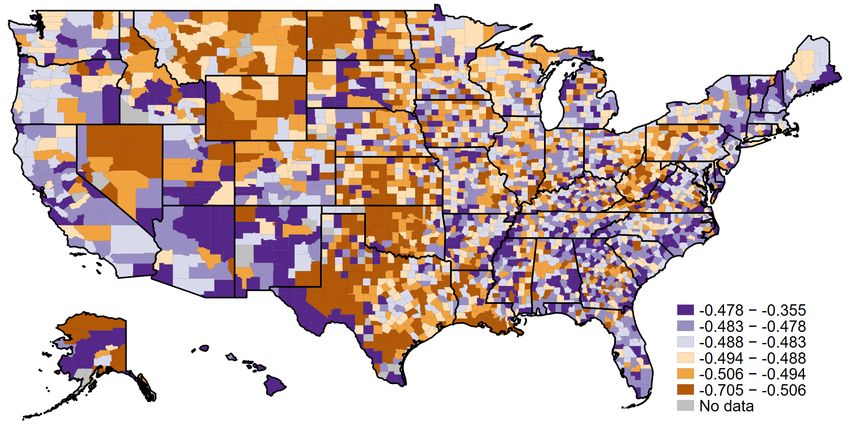
in market value of all firms in industry n attributable to COVID-19 exposure.28 As illustrated in
Figure 10, counties vary substantially in their weighted average changes in market value. Notably,
much of the “oil belt”, from Texas and Louisiana up through Oklahoma into Wyoming and North
Dakota, and parts of Pennsylvania – in brown – exhibit the largest declines. By contrast, much of
California and the East Coast – in blue – feature relatively lower declines. Interpreted through the
lens of Table 3, these trends indicate that the coasts have disproportionately large employment in
indutries containing labor-intensive firms.
Thus far, official estimates of job loss during the pandemic are available only in terms of initial
unemployment claims from the US Department of Labor, and only at the state level.29 Appendix
Figure A.7 displays the relationship between state changes in market value between January 22 and
April 10 (constructed in a manner analogous to counties above), and cumulative new jobless claims
per worker.30 This figure shows that states whose employment is more concentrated in industries
with milder losses in market value exhibit greater growth in jobless claims per worker.
As market value declines are larger in more labor-intensive industries (Figure A.5), this trend is
consistent with the idea that the labor-intensive sectors favored by the market shed relatively more
workers (vis a vis firms in capital-intensive sectors) in an effort to cut costs as consumption contracts
across the board (Baker et al., 2020), and revenues decline. Given the unprecedented collapse of
global economic activity, capital-intensive firms’ property, plant and equipment is effectively sunk.
As a consequence, firms that retain leverage on such assets may fare better by continuing to employ
26
As firm employment in COMPUSTAT is updated quarterly, we are at present unable to examine the link between
firm exposure to COVID-19 and firm employment directly. An additional complication is that firm employment data
in COMPUSTAT reflects worldwide, not just US employment. We will include this analysis as the data become
available.
27
We perform two checks on the representativeness of the publicly listed firms in our sample with respect to
employment. First, in appendix Figure A.5, we show that employment among these firms, while obviously different
in levels, is highly correlated across industries with US employment in 2016. Second, we find, in appendix Figure A.6,
that 95 percent of all counties have at least 76 percent of their employment in industries appearing among publicly
listed firms.
28
Country business pattern employment for 2016 are the latest available from Eckert et al. (2020). We show in
appendix Figures A.4 and A.4 that industries
with greater capital intensity exhibit greater declines in market value.
M Vj,t0 (1+r̂)52
P
j∈n
∆Ln(M
[ Vn ) = Ln M Vn,t0
is the market capitalization weighted average of return of all firms j in
industry n.
29
Initial jobless claims are available from the US Department of Labor website at https://oui.doleta.gov/
unemploy/claims_arch.asp. Current Employment Survey (CES) data available from the Bureau of Labor Statistics
(BLS) is not yet available for March, but will be included in a future draft.
30
That is, we sum the initial jobless claims from March 18 (before most of the COVID-19 labor market disruption
began) to April 11, and divide by the initial number of employees in the state according to the 2016 CBP.
17You can also read