Evaluation of Sentinel-1 and Sentinel-2 Feature Sets for Delineating Agricultural Fields in Heterogeneous Landscapes
←
→
Page content transcription
If your browser does not render page correctly, please read the page content below
Received July 12, 2021, accepted August 4, 2021, date of publication August 18, 2021, date of current version August 27, 2021.
Digital Object Identifier 10.1109/ACCESS.2021.3105903

Evaluation of Sentinel-1 and Sentinel-2 Feature
Sets for Delineating Agricultural Fields in
Heterogeneous Landscapes
GIDEON OKPOTI TETTEH 1 , ALEXANDER GOCHT 1 , STEFAN ERASMI1 ,
MARCEL SCHWIEDER1,2 , AND CHRISTOPHER CONRAD3
1 Thünen   Institute of Farm Economics, 38116 Braunschweig, Germany
2 Geography    Department, Humboldt University of Berlin, 10099 Berlin, Germany
3 Institute of Geosciences and Geography, Martin-Luther-University Halle-Wittenberg, 06099 Halle, Germany

Corresponding author: Gideon Okpoti Tetteh (gideon.tetteh@thuenen.de)

  ABSTRACT The Group on Earth Observations Global Agricultural Monitoring Initiative (GEOGLAM) con-
  siders agricultural fields as one of the essential variables that can be derived from satellite data. We evaluated
  the accuracy at which agricultural fields can be delineated from Sentinel-1 (S1) and Sentinel-2 (S2) images
  in different agricultural landscapes throughout the growing season. We used supervised segmentation based
  on the multiresolution segmentation (MRS) algorithm to first identify the optimal feature set from S1 and
  S2 images for field delineation. Based on this optimal feature set, we analyzed the segmentation accuracy
  of the fields delineated with increasing data availability between March and October of 2018. From the S1
  feature sets, the combination of the two polarizations and two radar indices attained the best segmentation
  results. For S2, the best results were achieved using a combination of all bands (coastal aerosol, water
  vapor, and cirrus bands were excluded) and six spectral indices. Combining the radar and spectral indices
  further improved the results. Compared to the single-period dataset in March, using the dataset covering the
  whole season led to a significant increase in the segmentation accuracy. For very small fields (< 0.5 ha),
  the segmentation accuracy obtained was 27.02%, for small fields (0.5 – 1.5 ha), the accuracy was 57.65%,
  for medium fields (1.5 ha – 15 ha), the accuracy was 75.71%, and for large fields (> 15 ha), the accuracy
  stood at 68.31%. As a use case, the segmentation result was used to aggregate and improve a pixel-based
  crop type map in Lower Saxony, Germany.

  INDEX TERMS Agricultural field delineation, band indices, essential agricultural variables, feature
  combination, image segmentation, intersection over union, remote sensing, segmentation optimization.

I. INTRODUCTION                                                                                 generated through the manual digitization of hardcopy maps
As part of its activities geared towards ensuring the attain-                                   (aerial images, topographic maps, etc.) [7] or direct field
ment of the United Nation’s Sustainable Development                                             measurements. The obvious problem with those approaches
Goals [1], the Group on Earth Observations Global Agricul-                                      is that they are costly and inefficient especially as agricultural
tural Monitoring Initiative (GEOGLAM1 ) identifies agricul-                                     maps require continuous updates to capture the real-time
tural fields as one of its essential agricultural variables [2].                                or near real-time events happening on agricultural fields.
Additionally, agricultural fields are valuable inputs to sub-                                   The use of remote sensing (RS) is a good alternative for
sequent processes such as crop type mapping [3], analysis                                       mapping agricultural fields given that satellite images can
of crop rotations [4], implementation of crop management                                        be acquired over wide geographical areas at a high temporal
activities [5], and the control of subsidy payments to                                          resolution [8]–[10].
farmers [6]. Conventionally, agricultural fields have been                                         The use of satellite images to delineate agricultural fields
                                                                                                has an extensive history in the RS world. It can largely
   The associate editor coordinating the review of this manuscript and                          be attributed to the use of medium spatial resolution satel-
approving it for publication was John Xun Yang .                                                lites like Landsat. For example, to extract agricultural
  1 https://earthobservations.org/geoglam.php (Accessed: Jul. 9, 2021).                         fields, numerous studies [7], [11]–[14] used the Landsat
                                           This work is licensed under a Creative Commons Attribution-NonCommercial-NoDerivatives 4.0 License.
116702                                                 For more information, see https://creativecommons.org/licenses/by-nc-nd/4.0/                  VOLUME 9, 2021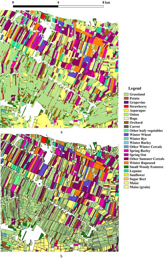
G. O. Tetteh et al.: Evaluation of Sentinel-1 and Sentinel-2 Feature Sets for Delineating Agricultural Fields

Thematic Mapper (TM), some [13]–[16] employed the Land-                                the segmentation algorithm has an impact on the segmenta-
sat Enhanced Thematic Mapper Plus (ETM+), and oth-                                     tion result. Therefore, it is worth exploring different S1 and
ers [17]–[20] used the Landsat 8 Operational Land Imager                               S2 feature sets to assess their impact on the segmentation of
(OLI). The common theme running through all of those stud-                             agricultural fields.
ies is the use of image segmentation as a means of extracting                             Beyond the feature set, agricultural fields are dynamic
the boundaries of the agricultural fields.                                             and change throughout the growing season, thereby requiring
   Image segmentation, which is the process of partition-                              continuous updates. Therefore, it is also relevant to analyze
ing an image into homogeneous and distinct objects, is the                             the accuracy at which the agricultural fields can be delineated
foundation of the object-based image analysis (OBIA)                                   from the S1 and S2 feature datasets at different times of the
paradigm [21]. The growth of the OBIA paradigm was                                     growing season. Further, it is important to assess the accuracy
fueled by the advent of high-resolution images and the avail-                          at which agricultural fields can be segmented from S1 and
ability of powerful computing environments [22]. It was                                S2 at different agricultural landscapes with different field
observed in [23] that the spatial resolution of an image has a                         sizes. In [2], the authors categorized three different field sizes:
direct impact on the outcome of image segmentation. In [5],                            small fields (< 1.5 ha), medium fields (1.5 ha – 15 ha),
the authors established that the higher the spatial resolution,                        and large fields (> 15 ha). They subsequently asserted that
the higher the coverage of agricultural fields eligible for site-                      medium spatial resolution images (here S1 and S2) are more
specific services like the monitoring of the Common Agricul-                           suitable for delineating large fields. Based on their respective
tural Policy (CAP) [24] and the application of smart farming                           spatial resolutions, S1 and S2 should be capable of spatially
technologies. Therefore, high or very high spatial resolution                          resolving small fields. For example, a 1 ha field should be
images are generally preferred for segmenting agricultural                             spatially resolved by S1 using 25 pixels and S2 using 100
fields. For example, pan-sharpened SPOT-5 images were                                  pixels. Therefore, the validity of the assertion in [2] ought to
used by [4], RapidEye by [25], WorldView-2/3 by [26],                                  be tested. Further, it remains to be seen what segmentation
QuickBird by [27], and digital orthophotos by [6]. However,                            accuracy can be achieved for those three field size categories.
for mapping large geographical areas, the use of high or very                             To fill all the aforementioned gaps, we set out in this
high spatial resolution images becomes infeasible as they                              study to execute the following objectives: (1) identify the
become extremely expensive to acquire. Therefore, medium                               optimal feature set from S1 and S2 images for segmenting
spatial resolution images remain the most viable option for                            agricultural fields, (2) analyze the evolution of the accuracy of
delineating agricultural fields at regional, national, and global                      agricultural fields segmented from the S1 and S2 feature sets
scales at little to no cost.                                                           throughout the growing season, and (3) assess the accuracy
   Although Landsat images have proven useful for mapping                              that can be achieved for different field sizes. To achieve our
agricultural fields over large areas, the spatial resolution                           objectives, we employed the multiresolution segmentation
of 30 m is often unable to resolve individual agricultural                             (MRS) algorithm [41] in eCognition [42] to segment agricul-
fields thereby inhibiting field-based applications in many                             tural fields from different feature sets generated from S1 and
cropping systems around the world [28]. Building on the                                S2 images acquired between March and October of 2018 in
experiences of the Landsat and SPOT missions, Sentinel-2                               Lower Saxony, Germany.
(S2) was designed within the framework of the European
Copernicus program for land surface and agriculture moni-                               II. STUDY AREA & DATA
toring [28] at a temporal resolution of 5 days and a spatial                            A. STUDY AREA
resolution of 10 m. As opposed to optical sensors, which are                           The federal state of Lower Saxony in Germany was selected
inhibited by clouds, Sentinel-1 (S1), which is also part of                            as the study area (Figure 1). Its total area of about
the Copernicus program enables the continuous monitoring                               4,770,041 ha has a mostly flat terrain and is located in the
of the earth’s surface in all weather conditions at a temporal                         temperate climate zone of Europe [36]. The majority of its
resolution of 6 days and a spatial resolution of 20 m. Various                         landmass is covered by agricultural lands that are mostly
researchers have used S1 [29], [30], and predominantly                                 dominated by grasslands, summer cereals, winter cereals,
S2 [31]–[40] for segmenting agricultural fields. In using the                          potatoes, winter rapeseed, and sugar beet [36]. For efficient
S1 or S2 images, most of those authors used existing segmen-                           segmentation purposes, the study area was divided into 575
tation algorithms (e.g., [29], [30], [32]–[34], [36]–[40]), some                       tiles. Each tile is 10 km by 10 km.
proposed new segmentation algorithms (e.g., [31], [35]), and                              To enable the smooth merger of the segmentation results
others proposed new segmentation parameter optimization                                from all the tiles, the geometry extent of each tile was
approaches (e.g., [36], [37]). One area that is yet to be com-                         extended or shrunk to cover the geometry of all poly-
prehensively explored is the determination of the optimal                              gons contained in the agricultural land-cover (LC) dataset
feature set from S1 and S2 images for segmenting agricultural                          (see Section II.C for the description of the dataset) whose
fields given that both sensors come with different bands and                           centroids intersected that particular tile. Consequently, the
additional features like band indices can be calculated as well.                       extended or shrunk tiles (symbolized as blue outlines
In an experiment based on a WorldView-2 image, the authors                             in Figure 1) have variable sizes with the average size
of [23] showed that the feature set used as the input to                               being 11 km by 11 km. To reduce the computation time

VOLUME 9, 2021                                                                                                                                     116703
G. O. Tetteh et al.: Evaluation of Sentinel-1 and Sentinel-2 Feature Sets for Delineating Agricultural Fields
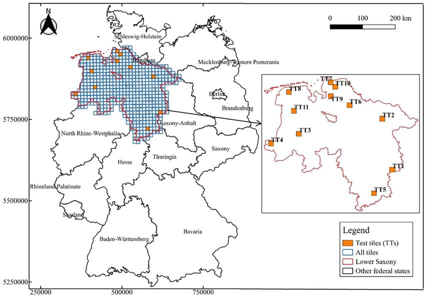
FIGURE 1. The study area (Lower Saxony) used in this study. A total of 575 tiles (blue outline) were created over Lower Saxony. The test
tiles (TTs) used as the basis to identify the optimal feature sets are symbolized in orange color. All the coordinates in the figure are in UTM
Zone 32N (EPSG:32632).
needed to identify the optimal feature set, we manually CARD-BS images, which come at a resampled spatial
assessed and selected eleven test tiles (TTs) (symbolized as resolution of 10 m, are generated by processing the Level-1
orange polygons in Figure 1) whose landscape compositions (L1) Ground Range Detected (GRD) images of S1 acquired in
were representative of the remaining tiles in Lower Sax- the Interferometric Wide Swath (IW) mode. The processing
ony. Details on how the selection was done are treated in is done by CODE-DE with the Sentinel Application Plat-
Section III.A. form (SNAP) using the standard procedure of applying an
orbit file, removing GRD border noise, removing thermal
B. SATELLITE DATA noise, calibration, and terrain correction [44].
A recent study [43] demonstrated the usability of monthly For S2, we used FORCE (Framework for Operational
composites of S1 and S2 images for large-scale mapping Radiometric Correction for Environmental monitoring) [45].
of agricultural land-use (LU) types. For our study, we used FORCE is a processing software for generating higher-level
monthly mean composites (MMCs) of S1 and S2 images from analysis-ready data (ARD) from S2 and Landsat images.
March to October 2018. For the MMCs of S1, we downloaded Based on the top-of-atmosphere L1C images of S2, FORCE
the Sentinel-1 L3 BS (Sentinel-1 Level-3 Backscatter) data generates bottom-of-atmosphere L2 ARD images by correct-
from CODE-DE (Copernicus Data and Exploitation Platform ing for atmospheric, geometric, and bidirectional reflectance
– Deutschland).2 CODE-DE is a cloud computing platform distribution function (BRDF) effects [46]–[48]. In FORCE,
that provides access to the datasets of the Copernicus program clouds and cloud shadows are detected and masked using
covering Germany as well as virtual machines for data pro- the Fmask algorithm [49]–[51]. The cloud and cloud shadow
cessing. The Sentinel-1 L3 BS images in VV and VH polar- pixels were replaced using an interpolation method based
izations are created by averaging all the Sentinel-1 L2 on an ensemble of radial basis function (RBF) convolution
CARD-BS (Sentinel-1 Level-2 Copernicus Analysis Ready filters [52]. FORCE outputs all S2 bands except the ones with
Data – Backscatter) images over a month. The Sentinel-1 L2 a spatial resolution of 60 m, i.e., the coastal aerosol, water
vapor, and cirrus bands. The bands with a spatial resolution
2 https://code-de.org/en/ (Accessed: Jul. 9, 2021). of 20 meters are resampled to 10 m. For each band, all pixel
116704 VOLUME 9, 2021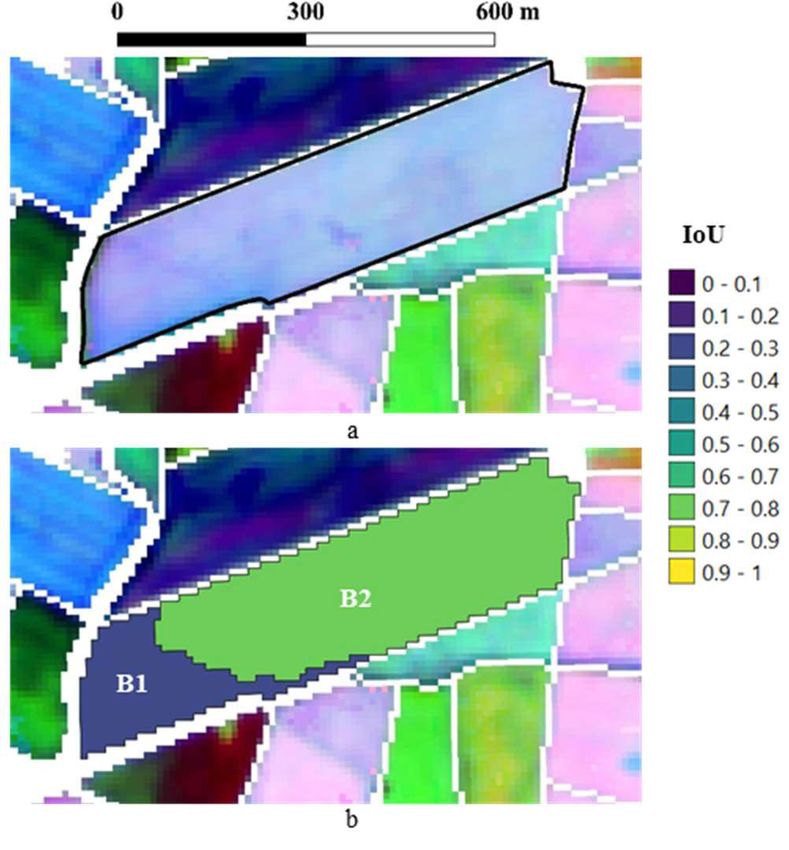
G. O. Tetteh et al.: Evaluation of Sentinel-1 and Sentinel-2 Feature Sets for Delineating Agricultural Fields
values belonging to the same month were averaged to obtain
the MMCs for S2.
C. AGRICULTURAL LAND-COVER
From the digital landscape model of the German Offi-
cial Topographic Cartographic Information System (ATKIS)
of 2018, we extracted the vector layer containing polygons
of the agricultural LC (arable land and grassland) present at
the tiles. This layer was used to create a mask to remove
non-agricultural areas from the MMC images before seg-
menting the agricultural fields. This approach has also been
used in other studies [31], [36], [37].
D. REFERENCE DATA
For segmentation evaluation and optimization, we used the
Geospatial Aid Application (GSAA) data of 2018 covering FIGURE 2. The workflow we followed in this study.
the TTs. This data was obtained from the Lower Saxony
Ministry of Food, Agriculture, and Consumer Protection. The where X is a GSAA parcel. For each tile, the SF factor is
GSAA data contains the boundaries of agricultural parcels calculated for all GSAA polygons. Higher SF values indi-
manually digitized from very high-resolution orthoimages cate more compact polygons, while lower values represent
(spatial resolution ≤ 1 m) by farmers intending to access more elongated or irregular-shaped polygons. The selected
the subsidies within the CAP framework. The LU type (e.g., tiles have variable SF distributions as captured by Figure 15
mowing pasture, meadow, maize, winter wheat, etc.) of each (Appendix A).
agricultural parcel is additionally declared by the farmer. The
average size of an agricultural parcel over the TTs is about B. BAND INDICES
3.4 ha, with the minimum size being about 0.2 ha and the Eight band indices (two radar and six optical) (Table 1) with
maximum size being about 63 ha. The average number of extensive usage in RS for mapping agricultural lands were
agricultural parcels per tile is 2,463. For each test tile, basic used in this study. The radar and optical indices were com-
descriptive information of the GSAA parcels can be found puted using the MMC images of S1 and S2, respectively. All
in Table 5 of Appendix A. the indices required at least two bands for computation. Given
that the S2 MMC images had ten bands, the optical indices
III. METHODOLOGY were selected to cover different parts of the electromagnetic
The workflow we used in this study is depicted in Figure 2. spectrum as was previously done in [3]. The S1 MMC images
The components of the workflow will be explained in the next come with only two bands, hence each radar index used both
subsections. bands for computation.
A. SELECTION OF TEST TILES (TTs)
C. CLIPPING AND MASKING
The selection of the TTs was based on four criteria namely a
high percentage coverage of agricultural LU, a high number Each MMC and band index of S1 and S2 was clipped to the
of reference parcels for segmentation evaluation, the pres- boundary of a test tile. After clipping, all non-agricultural
ence of both big and small agricultural fields, and a variable areas were removed. The agricultural vector layer extracted
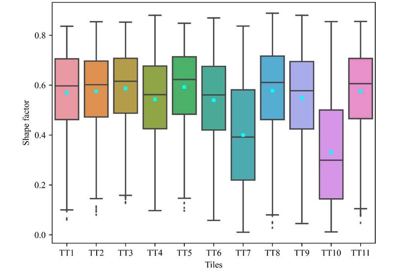
shape factor (SF) distribution per tile. The selected TTs are from ATKIS was used for this purpose. This vector layer con-
more dominated by agricultural LU as depicted in Figure 14 tains cadastral polygons of all agricultural lands in Germany.
(Appendix A). Each selected tile contains a mixture of both We applied a negative buffer distance of 5 m to each polygon
big and small fields (see Table 5 of Appendix A). The to create a separation between two adjacent polygons that
authors in [36] and [53] emphasized the importance of hav- share a common boundary. The reason for the negative buffer
ing a sizeable number of reference objects for supervised was to ensure the ease of separation between adjacent agricul-
segmentation evaluation to ensure accurate results. In our tural fields in the images during the segmentation process. All
study, the minimum number of reference fields was 1,622 at pixels outside the buffered polygons were masked out from
TT2, which we considered as a sizeable number. The SF each MMC and band index. These masked images were used
was used to quantify the shape characteristics of the GSAA for all subsequent processes.
parcels within each tile. We adopted the SF method in (1) as
was proposed by [54]; D. GENERATE FEATURE SETS
A feature set is a combination of two or more features (bands,
4 ∗ 5 ∗ Area (X ) indices). In all, nine feature sets were created (Table 2). The
SF = (1)
(Perimeter (X ))2 table shows each feature set alongside the input features that
VOLUME 9, 2021 116705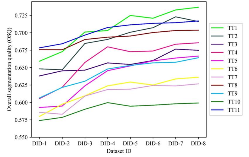
G. O. Tetteh et al.: Evaluation of Sentinel-1 and Sentinel-2 Feature Sets for Delineating Agricultural Fields

TABLE 1. The utilized radar and optical indices, abbreviations, formulas,        feature dataset. Nine seasonal feature datasets were created
and sources in the literature.
                                                                                 per tile. To optimize the segmentation of those nine seasonal
                                                                                 feature datasets per tile, we used the supervised segmentation
                                                                                 optimization (SSO) approach of [36]. That SSO approach
                                                                                 utilizes the MRS algorithm. Given that the MRS algorithm
                                                                                 requires three main parameters (scale, shape, and compact-
                                                                                 ness), all of which take a varied range of input values, that
                                                                                 SSO approach uses Bayesian optimization to identify the sin-
                                                                                 gle parameter combination that yields the optimal segmenta-
                                                                                 tion output. The accuracy of the segmentation output of each
                                                                                 parameter combination is measured through the overall seg-
                                                                                 mentation quality (OSQ) metric, which is an area-weighted
                                                                                 average of the Jaccard index [63]. The Jaccard index, which is
                                                                                 widely known as Intersection over Union (IoU), is frequently
                                                                                 used in computer vision tasks to measure the geometric simi-
                                                                                 larity between a reference object and a target object extracted
                                                                                 from an image or a video. The formula for IoU and OSQ as
                                                                                 culled from [36] is given in (2) and (3), respectively;

                                                                                                           Area (X ∩ Y )
                                                                                                 IoU (Y ) =                                                    (2)
                                                                                                           Area (X ∪ Y )
                                                                                                           Pn
                                                                                                             i=1 Area(Yi ) ∗ IoU (Yi )
                                                                                                     OSQ =      Pn                                             (3)
                                                                                                                  i=1 Area(Yi )
TABLE 2. The nine feature sets used for optimization: data sources,
names, and lists of input features.                                              where X is a reference object, Y is its target object (segment),
                                                                                 X ∩Y is the spatial intersection between them, X ∪Y repre-
                                                                                 sents their spatial union, and n is the total number of segments
                                                                                 in a segmentation output. Given an input image and a refer-
                                                                                 ence dataset (GSAA in our case), the SSO approach uses 150
                                                                                 parameter combinations and then returns the segmentation
                                                                                 output that best matches the reference data. It also returns
                                                                                 the corresponding OSQ value as well as the IoU value of
                                                                                 each segment in the optimal segmentation output. Both IoU
                                                                                 and OSQ range from zero (lowest segmentation quality) to
                                                                                 one (highest segmentation quality). The feature set with the
                                                                                 highest average OSQ over the eleven tiles was adjudged as
                                                                                 the best.

                                                                                 F. EVALUATE THE EVOLUTION OF SEGMENTATION
                                                                                 ACCURACY OVER TIME
                                                                                 To assess the evolution of the segmentation accuracy of
were used to create it. Three feature sets were based on S1 and                  agricultural fields over time, we created incremental feature
five were based on S2. Those S1 and S2 feature sets were                         datasets covering different months of the growing season
created after conducting some pretests to assess the separate                    based on the optimal feature set identified in section III.E.
impact of the bands and band indices on the segmentation                         Table 3 shows how the incremental feature datasets were
accuracy. During the conduction of the pretests, we realized                     created. The first incremental feature dataset (DID-1) was
that a combination of the radar and optical indices led to                       created using the feature dataset of March only. The one in
an increase in the segmentation accuracy, hence the creation                     April (DID-2) contains the feature datasets of March and
of the combined feature set named S2S1I. Based on each                           April. This incremental process continued up to October
feature set, a feature dataset was generated for each month                      (DID-8). DID-8 is the same as a seasonal feature dataset
in the growing season using the masked images created in                         described in section III.E. The number of bands in each incre-
section III.C.                                                                   mental feature dataset varied. Assuming S2B4 was estab-
                                                                                 lished as the optimal feature set, DID-1 will have four bands,
E. IDENTIFY OPTIMAL FEATURE SET                                                  DID-2 will contain eight bands, and DID-8 will have 32
For each feature set in Table 2, all feature datasets from                       bands. For each of the eleven tiles, eight incremental fea-
March to October were stacked together to create a seasonal                      ture datasets were created. Each incremental feature dataset

116706                                                                                                                                             VOLUME 9, 2021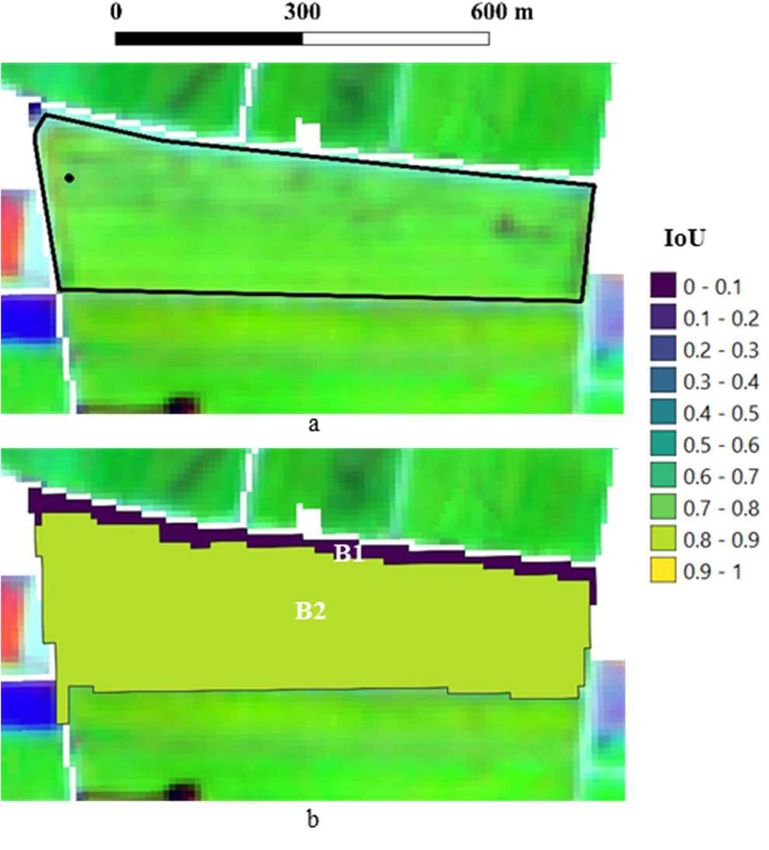
G. O. Tetteh et al.: Evaluation of Sentinel-1 and Sentinel-2 Feature Sets for Delineating Agricultural Fields

TABLE 3. The incremental feature datasets (DID-1 to DID-8) that were                   segments with better geometric matches to the GSAA parcels
created in this study. The ‘‘x’’ symbol means that the feature dataset of
that month was used in creating the incremental feature dataset.                       than the other feature sets, which resulted in it obtaining the
                                                                                       highest average OSQ. Compared with S2B10I and S2S1I,
                                                                                       the higher values for low-IoU bins obtained by S1BI as shown
                                                                                       in Figure 5 explain its low accuracies in Figure 3 and Figure 4.
                                                                                          Based on the best feature set (S2S1I), we visually inspected
                                                                                       the optimal segmentation results at TT1 (highest OSQ
                                                                                       of 73.7%) and TT10 (lowest OSQ of 59.9%) to understand
                                                                                       the reasons behind the difference in OSQ between them.
                                                                                       Figure 6 shows the segmentation results achieved at TT1 and
                                                                                       TT10. The false-color image of S2S1I at TT1 and TT10 are
                                                                                       depicted in Figure 6a and Figure 6b, respectively. The GSAA
                                                                                       parcels (black outlines) have been overlaid on the false-color
                                                                                       images in Figure 6c and Figure 6d, respectively. The optimal
                                                                                       segments symbolized by their respective IoU values have
served as an input to the SSO approach and the corresponding                           been overlaid on the false-color images in Figure 6e and
results were recorded.                                                                 Figure 6f, respectively. The segments that touch the bound-
                                                                                       aries of each tile are excluded in the SSO approach because
IV. RESULTS                                                                            they are artifacts, hence they are not displayed in Figure 6e
A. OPTIMAL FEATURE SET FOR SEGMENTATION                                                and Figure 6f. The reason for the difference in OSQ between
Figure 3 shows the variability of OSQs obtained at the eleven                          those two tiles is attributable to the difference in the size
TTs for each feature set as well as the average OSQ (cyan                              and shape of agricultural fields at each tile. At TT1, the tiles
boxes) obtained by each feature set over the test tiles. The                           are bigger and more compact. The opposite can be seen at
S1 feature set based on only the radar indices (S1I) out-                              TT10, where most of the agricultural fields are smaller and
performed the one based on only the radar bands (S1B).                                 less compact (more elongated).
The combination of the radar bands and indices (S1BI) led
to an increase in OSQ. The feature set purely based on
the S2 indices (S2I) outperformed those purely based on                                B. EVOLUTION OF SEGMENTATION ACCURACY OVER
the spectral bands (S2B4, S2B10). The combination of the                               TIME
S2 bands and S2I to respectively create S2B4I and S2B10I                               The average OSQ attained by each S2S1I-based incremental
improved the segmentation results as compared to separately                            feature dataset over all tiles is depicted in Figure 7. The lowest
using either S2B4 or S2B10. Among the feature sets based on                            OSQs were mostly obtained at the beginning of the growing
only the S2 bands, S2B4 yielded better results than S2B10.                             season in March with DID-1. As the season progressed and
The combination of the S2 and S1 indices (S2S1I) obtained                              more datasets were acquired and used, the segmentation accu-
the highest average OSQ. The numerical values of the average                           racy increased accordingly. The highest OSQs were mostly
OSQs obtained by the feature sets over all the test tiles are                          achieved at the end of the growing season in October (DID-8).
reported in Table 6 of Appendix A.                                                     As Figure 8 shows, the optimal OSQ at eight tiles (TT1, TT4,
   The breakdown of the performance of each feature set per                            TT5, TT6, TT7, TT8, TT9, TT11) was attained with DID-8,
tile is shown in Figure 4. S2S1I yielded the best results at                           two tiles (TT2, TT3) with DID-7, and one tile (TT10) with
three tiles (TT3, TT4, TT10), S2B10I at three tiles (TT2, TT8,                         DID-4. The difference in average OSQ of 5.31 percentage
TT11), S1BI at two tiles (TT1, TT5), S1I at two tiles (TT6,                            points between DID-1 (62.2%) and DID-8 (67.51%) was
TT7), and then S2B4I at one tile (TT9).                                                observed to be statistically significant (p-value = 0.006)
   The optimal parameter combinations associated with S1BI                             based on a two-tailed t-test. In the incremental segmentation
(optimal among the S1 feature sets), S2B10I (optimal among                             set-up, the highest improvement in OSQ of almost 2% was
the S2 feature sets), and S2S1I (overall optimal feature set)                          achieved by adding the May dataset to the incremental stack
per tile are shown in Table 7 of Appendix A.                                           to create DID-3. This was followed by the addition of the June
   To understand the differences in OSQ between the fea-                               dataset to create DID-4, which led to an increase of about
ture sets, we further investigated S1BI, S2B10I, and S2S1I.                            1.2%. After June, the increase became more gradual.
We generated the area-weighted histogram in Figure 5 with                                 We used the IoU values of the segments in the optimal
ten bins using the IoU computed for each segment in the                                segmentation results generated with the incremental feature
optimal segmentation results that were respectively obtained                           datasets to create the area-weighted histogram shown in
by S1BI, S2B10I, and S2S1I at all test tiles. We created                               Figure 9, which focuses on DID-1 (start of the season), DID-3
an area-weighted histogram because the OSQ is also area-                               (after the farmers submit their GSAA), and DID-8 (end of
weighted. To create the histogram, each IoU contributed its                            the season). The optimal segmentation results respectively
segment area to the bin count (frequency) instead of one.                              obtained with DID-3 and DID-8 produced more segments that
As the histogram shows, the S2S1I feature set generated more                           geometrically matched the GSAA parcels than DID-1 did.

VOLUME 9, 2021                                                                                                                                    116707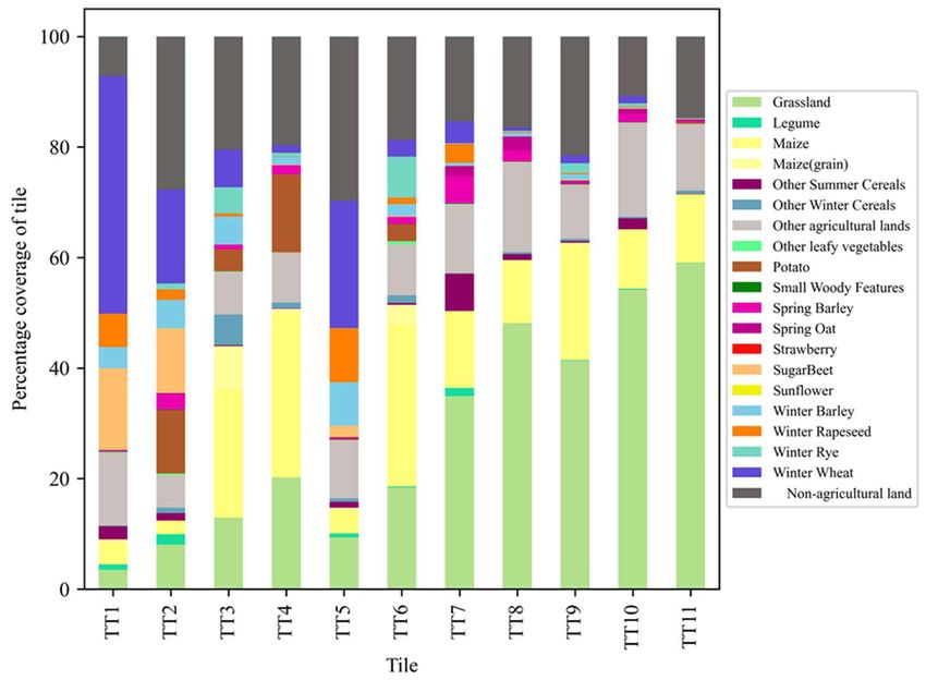
G. O. Tetteh et al.: Evaluation of Sentinel-1 and Sentinel-2 Feature Sets for Delineating Agricultural Fields

               FIGURE 3. Boxplots showing the variability of OSQs obtained at the eleven tiles per feature set. The cyan boxes
               represent the average OSQs achieved by each feature set over the tiles. The within-box horizontal lines are the
               median OSQs. The black dots are the OSQs that are outliers.

             FIGURE 4. The OSQ obtained by each feature set per tile.

C. PLAUSIBILITY ANALYSIS: COMPARISON OF THE                                  In Figure 10a, the GSAA parcel indicates the presence of a
SEGMENTATION RESULTS WITH THE GSAA PARCELS                                   single LU (mowing pasture) but due to the inward buffer
In [36], over-segmentation was identified as the main rea-                   applied at the masking stage, an artificial boundary was cre-
son for the disparity between the GSAA parcels and the                       ated in the satellite image leading to the incorrect generation
segmentation results. In addition to the instances of over-                  of two separate segments (B1, B2) as shown in Figure 10b.
segmentation established in [36], we identified a new instance               B1 and B2 had moderate IoU values of 51% and 35.9%,
of over-segmentation, which was caused by the masking                        respectively. A higher IoU value could have been achieved
approach we used in this study as shown in Figure 10.                        with a single segment without any separation between them.

116708                                                                                                                                         VOLUME 9, 2021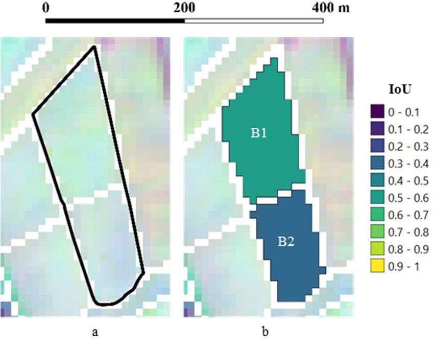
G. O. Tetteh et al.: Evaluation of Sentinel-1 and Sentinel-2 Feature Sets for Delineating Agricultural Fields

           FIGURE 5. Area-weighted histogram of the Intersection over Union (IoU) values computed for the segments in the optimal
           segmentation results achieved respectively by S1BI, S2B10I, and S2S1I at all test tiles.

TABLE 4. Overall segmentation quality (OSQ) computed for the different                 as shown in Figure 11 and Figure 12, where the size of
field size categories.
                                                                                       the GSAA parcels are 19.6 ha and 15.7 ha, respectively.
                                                                                       To receive the greening payments within CAP, farmers with
                                                                                       arable land exceeding 15 ha have to use at least 5% of their
                                                                                       land as an Ecological Focus Area (EFA), e.g., hedges. Due
                                                                                       to the presence of hedges in Figure 11a, the SSO correctly
                                                                                       created one segment containing the hedges (B1) and a second
                                                                                       segment without hedges (B2) as captured in Figure 11b.
                                                                                       Unfortunately, B1 had a low accuracy of 6.4%. B2 was 86.4%
D. SEGMENTATION ACCURACY FOR DIFFERENT FIELD
                                                                                       accurate. In Figure 12, although the image (Figure 12a) looks
SIZES
                                                                                       relatively homogenous, two separate segments (B1 and B2)
                                                                                       with respective accuracies of 21.3% and 73.9 % were created
The segmentation optimization process was subsequently
                                                                                       by the SSO as shown in Figure 12b. This is an error caused
extended to the other tiles in Lower Saxony based on the
                                                                                       by the MRS parameters not being optimal for that particular
DID-8 generated for S2S1I. The optimal segmentation results
                                                                                       agricultural field, even though the identified parameters were
of the 575 tiles were then merged. The merged result can
                                                                                       optimal for the tile that contains that field.
be viewed as the ‘‘original_segmentation_ni’’ layer on this
web map.3 Based on this merged result, we analyzed the
                                                                                       E. USE CASE: POST-FILTERING OF PIXEL-BASED CROP
impact of the area of the agricultural fields on the OSQ.
                                                                                       MAPS
In [5], the authors stated that a minimum of 50 pixels per
field is the critical number required for site-specific smart                          In [64], the authors showed that the post-filtering of pixel-
farming. Therefore, we separated the small field size category                         based crop type maps using image segments through majority
of [2] into two sub-groups: very small fields (< 0.5 ha) and                           voting can improve image classification results. Therefore,
small fields (0.5 ha – 1.5 ha). The medium and large field                             as a use case, we tested if the crop type map of [65] as
categories were kept. Table 4 shows the OSQ computed for                               visualized on this webpage4 could be improved using the
each category.                                                                         merged segmentation result of Lower Saxony. Before pro-
   From Table 4, the accuracy of large fields was lower than                           ceeding with this test, we first post-processed the merged
the medium fields. A visual assessment of the results revealed                         segments in GRASS GIS. 5 We applied ‘‘v.clean’’ to first
some of the instances that contributed to that phenomenon                                4 https://ows.geo.hu-berlin.de/webviewer/croptypes/ (Accessed: Jul. 9,
                                                                                       2021).
  3 https://tisdex.thuenen.de/maps/34/view#/ (Accessed: Jul. 9, 2021).                   5 https://grass.osgeo.org/ (Accessed: Jul. 9, 2021).

VOLUME 9, 2021                                                                                                                                         116709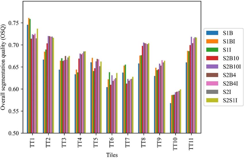
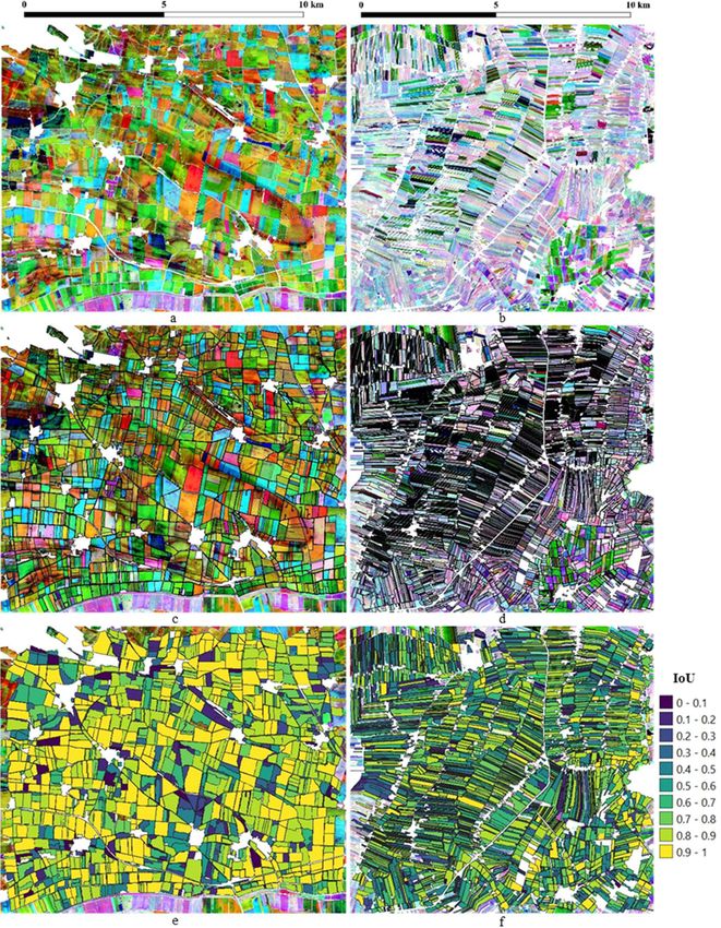
G. O. Tetteh et al.: Evaluation of Sentinel-1 and Sentinel-2 Feature Sets for Delineating Agricultural Fields

  FIGURE 6. Optimal segmentation results obtained at TT1 (left column) and TT10 (right column) based on S2S1I. (a) and (b) show the false-color
  composites of the NDVI MMCs of March, June, and October. The GSAA parcels (black outlines) have been overlaid on the respective images at
  (c) and (d). The optimal segments have been symbolized with their corresponding IoU values and subsequently draped over each image at
  (e) and (f), respectively. The geographical extent of TT1 is roughly 12.3 km by 10.3 km and that of TT10 is roughly 11.3 km by 10.7 km.

116710                                                                                                                                           VOLUME 9, 2021
G. O. Tetteh et al.: Evaluation of Sentinel-1 and Sentinel-2 Feature Sets for Delineating Agricultural Fields

                        FIGURE 7. Boxplots showing the variability of OSQs obtained at the eleven tiles by the S2S1I-based
                        incremental feature datasets. The cyan boxes are the average OSQs over all tiles as obtained by the
                        incremental feature datasets. The within-box horizontal lines are the median OSQs.

                  FIGURE 8. The OSQ obtained by each S2S1I-based incremental feature dataset per tile.

remove duplicate segments created due to overlapping tiles                             the majority vote was a smoothed map, where most of the
and then applied ‘‘v.generalize’’ to simplify the segments.                            noise in the pixel-based map had been removed. An accuracy
The simplified segments can be viewed as the ‘‘simpli-                                 assessment performed using all the GSAA parcels of Lower
fied_segmentation_ni’’ layer in this web map.6 We subse-                               Saxony indicated an improvement in the overall accuracy
quently applied a majority vote filter to determine the crop                           after filtering from 78% to 81.4% and the Kappa statistic from
type of each segment. As an example, the pixel-based crop                              0.705 to 0.747.
type map and the crop type map after the majority vote at TT7
(balanced share of arable lands and grasslands) are captured                            V. DISCUSSION
by Figure 13a and Figure 13b, respectively. The outcome of                             This current study builds on the previous work of [36].
                                                                                       In [36], the authors only focused on the development of
  6 https://tisdex.thuenen.de/maps/34/view#/ (Accessed: Jul. 9, 2021).                 the optimization approach. No attention was given to the

VOLUME 9, 2021                                                                                                                                116711
G. O. Tetteh et al.: Evaluation of Sentinel-1 and Sentinel-2 Feature Sets for Delineating Agricultural Fields
FIGURE 9. Area-weighted histogram of the Intersection over Union (IoU) values computed for the segments in the optimal
segmentation results achieved respectively by DID-1, DID-3, and DID-8 at all test tiles.
FIGURE 10. Over-segmentation caused by the masking approach used in
this study. The background displays in (a) and (b) are based on the
false-color image created for DID-8 using the NDVIs of March, June, and
October. The image in (a) has been overlaid with the GSAA parcel (black
outline). The corresponding segments generated are symbolized in (b) by
their IoU values. Two separate segments labeled B1 and B2 were created.
FIGURE 11. Over-segmentation caused by hedges. The background
identification of the optimal feature set for segmenting the displays in (a) and (b) are based on the false-color image created for
agricultural fields. In [36], cloud-free S2 images were man- DID-8 using the NDVIs of March, June, and October. The image in (a) has
ually selected and used. In this study, an automated pro- been overlaid with the GSAA parcel (black outline). The LU of this GSAA
parcel is potato. The corresponding segments generated are symbolized
cess based on FORCE was used to identify and replace in (b) by their IoU values. Two separate segments labeled B1 and B2 were
clouds. This study also evaluated pre-processed S1 datasets created.
as obtained from CODE-DE. For our current study, we used
monthly composites of S1 and S2 unlike [36], where single- categories was not assessed. Finally, in this study, the use of
date S2 images were used. In [36], the segmentation accuracy image segmentation to aggregate and improve a pixel-based
that could be achieved for different agricultural field size crop type map was evaluated.
116712 VOLUME 9, 2021G. O. Tetteh et al.: Evaluation of Sentinel-1 and Sentinel-2 Feature Sets for Delineating Agricultural Fields
the speckle noise, thereby revealing the boundaries of agri-
cultural fields. The masking approach used in this study
was potentially more beneficial to S1 in creating boundaries
between adjacent fields. In situations where S2 images are
not available due to clouds, monthly composites of S1 images
could be used for segmenting agricultural fields. Overall,
the combination of S1 and S2 resulted in the highest segmen-
tation accuracy (Figure 3). Within the context of mapping
agricultural LU types, other authors [43], [69], [70] also
observed that combining S1 and S2 leads to better results than
separately using each sensor.
Based on the seasonal feature dataset (DID-8) created from
the combined S1 and S2 feature set, the highest OSQ occurred
at TT1 (Figure 6e) and the lowest at TT10 (Figure 6f).
The main driving forces behind the obtained OSQs were
the area and shape of agricultural fields at the tiles. Due
to the presence of big and compact agricultural fields at
TT1, the segmentation process was more successful there.
At TT10, most of the agricultural fields are small and elon-
gated, and additionally, they are highly dominated by one LU
(mowing pasture). Such conditions coupled with the spatial
resolution of S1 and S2 make it difficult to appropriately
FIGURE 12. Over-segmentation caused by the non-optimal MRS
parameters. The background displays in (a) and (b) are based on the
segment agricultural fields from S1 and S2 images because
false-color image created for DID-8 using the NDVIs of March, June, and clear-cut boundaries between agricultural fields cannot be
October. The image in (a) has been overlaid with the GSAA parcel (black distinguished in the S1 and S2 images. This observation was
outline). The LU of this GSAA parcel is mowing pasture. The
corresponding segments generated are symbolized in (b) by their IoU also made by [36] in their research as they encountered a
values. Two separate segments labeled B1 and B2 were created. similar problem. The use of an image with a higher spatial
resolution than S2 was proposed by [36] as a likely solution.
For segmenting agricultural fields, using only the visible Because agricultural fields are dynamic and change over
and near-infrared bands (S2B4) of S2 was superior to using time, to accurately map different agricultural LU types,
all ten bands (S2B10) as depicted in Figure 3. A similar the use of multitemporal images is considered a requirement
outcome was reported by [23], who received more accurate by [71]. With multitemporal images, the different phenolog-
results using only the visible (RGB) bands of a Worldview- ical behaviors of different agricultural LU types throughout
2 image as compared to using all the eight bands for image the growing season can be characterized and effectively used
segmentation based on the MRS algorithm. They attributed to differentiate them [72]. Although that suggestion was made
this phenomenon to the high correlation existing between the within the context of image classification, it also applies to
eight bands. To deal with this problem, they applied principal the segmentation of agricultural fields as was highlighted by
component analysis (PCA) to the eight bands and used the these authors [39], [73]. As Figure 7 shows, using a single-
first three components for segmentation. The result was better period dataset (DID-1) resulted in segments with signifi-
than using all eight bands but underperformed in comparison cantly lower accuracies than those created using the dataset
with the RGB bands. In using S2, most authors [33]–[40] covering the whole growing season (DID-8). This demon-
directly used S2B4 to segment agricultural fields without strates the importance of using multitemporal images for the
testing other feature combinations. The superiority of S2B4 to effective segmentation of agricultural fields. Consecutively
S2B10 as established in this study validates the choice of increasing the number of images (S2S1I in our case) led
S2B4 by those authors for segmenting agricultural fields. to a corresponding increase in the segmentation accuracy
Due to the inherently speckled nature of radar images, (Figure 7). Although these studies [74], [75] were exclu-
some researchers [66]–[68] have asserted that the segmen- sively focused on object classification, they also observed a
tation of optical images is easier and more accurate. Their similar phenomenon, in that, increasing the number of input
assertion can largely be backed by Figure 3, where most of images yielded an increase in the accuracy of the classified
the feature sets based on only S2 outperformed those based on segments.
only S1. However, the S1 feature sets (S1I, S1BI) containing Some sources of error identified in this study included
the radar indices proved capable of segmenting agricultural the masking approach, which led to the over-segmentation
fields even to the extent that they outperformed S2B10. The captured in Figure 10. This problem could be resolved by
speckle noise in radar images often makes it difficult to visu- using an improved agricultural LC dataset. Another source of
ally identify the boundaries of features. Monthly compositing error was the presence of hedges in the images, which led to
was particularly beneficial to S1 as it helped in reducing low segmentation accuracies as was highlighted in Figure 11.
VOLUME 9, 2021 116713G. O. Tetteh et al.: Evaluation of Sentinel-1 and Sentinel-2 Feature Sets for Delineating Agricultural Fields
FIGURE 13. Usage of a majority vote to generate an object-based crop type map (b) from the
pixel-based crop type map (a).
Although the presence of the hedge led to a low segmentation One solution will be to apply the segmentation optimization
accuracy, such segmentation errors are acceptable especially based on each GSAA parcel instead of using all parcels within
for subsequent processes like crop type mapping meant to a tile for the optimization. However, such an approach will be
determine the actual LU within a field. The last source of computationally expensive. A more efficient solution will be
error as highlighted in Figure 12 was caused by the non- to merge neighboring segments with the same LU type after
optimal MRS parameters. The segmentation optimization in object classification as was proposed by [36]. After applying
this study was applied to roughly 11 km by 11 km tiles. the majority vote filter, both segments in Figure 12b were
In tiles with predominantly smaller fields, such instances of classified as grasslands, hence they could be merged as one
over-segmentation as displayed in Figure 12 are unavoidable. segment.
116714 VOLUME 9, 2021G. O. Tetteh et al.: Evaluation of Sentinel-1 and Sentinel-2 Feature Sets for Delineating Agricultural Fields
FIGURE 14. Distribution of land-use (LU) per tile.
FIGURE 15. The boxplots showing the distribution of shape factors (SFs) per tile. The cyan boxes represent the average SFs. The within-box
horizontal lines are the median SFs.
VOLUME 9, 2021 116715G. O. Tetteh et al.: Evaluation of Sentinel-1 and Sentinel-2 Feature Sets for Delineating Agricultural Fields
TABLE 5. Basic descriptive information of the GSAA parcels used in this TABLE 7. The optimal parameter combinations obtained by S1BI (optimal
study per test tile. among the S1 feature sets), S2B10I (optimal among the S2 feature sets),
and S2S1I (overall optimal feature set) per tile.
TABLE 6. The average OSQs obtained by each feature set over the eleven
test tiles.
The general trend discernable from Table 4 is that
bigger fields lead to higher segmentation accuracies as
was also established in [36]. Contrary to the suggestion
of [2] that S1 and S2 are more suitable for large fields,
Table 4 rather showed that the S1 and S2 images are
more suitable for medium fields. The larger the fields,
the higher the probability of over-segmentation as was
depicted in Figure 11 and Figure 12, both of which led to
lower segmentation accuracies.
The usefulness of image segmentation for post-filtering
pixel-based crop type maps was briefly demonstrated in results from the eleven test tiles, the segmentation optimiza-
this study. The derived object-based map was more visually tion process was extended to every part of Lower Saxony.
appealing and also increased the classification accuracy. The results obtained in this study allow for the following
conclusions to be drawn: (1) S2 generally yields better seg-
VI. CONCLUSION mentation results than S1, (2) the synergistic use of S1 and
In this study, we applied supervised segmentation optimiza- S2 can lead to an improvement in segmentation accuracy,
tion to different feature datasets generated from S1 and (3) multitemporal S1 and S2 images are key to the optimal
S2 images at eleven test tiles in Lower Saxony, Germany segmentation of agricultural fields, (4) S1 and S2 images are
to identify the optimal feature set for segmenting agricul- more suitable for segmenting medium-sized (1.5 – 15 ha)
tural fields. Additionally, the accuracy of agricultural fields agricultural fields, and (5) post-filtering of pixel-based crop
segmented from the S1 and S2 feature datasets between type maps with agricultural fields extracted via image seg-
March and October of 2018 was analyzed. Based on the mentation improves classification accuracies.
116716 VOLUME 9, 2021G. O. Tetteh et al.: Evaluation of Sentinel-1 and Sentinel-2 Feature Sets for Delineating Agricultural Fields
The main outcome (agricultural fields) of this study can [6] A. García-Pedrero, M. Lillo-Saavedra, D. Rodríguez-Esparragón, and
be used to produce object-based crop type maps. An object- C. Gonzalo-Martín, ‘‘Deep learning for automatic outlining agricultural
parcels: Exploiting the land parcel identification system,’’ IEEE Access,
based crop type map is useful for subsequent processes like vol. 7, pp. 158223–158236, 2019, doi: 10.1109/ACCESS.2019.2950371.
the correct estimation of the area per crop type, crop yield [7] C. Y. Ji, ‘‘Delineating agricultural field boundaries from TM imagery using
modeling, crop rotation analysis, greenhouse gas (GHG) dyadic wavelet transforms,’’ ISPRS J. Photogramm. Remote Sens., vol. 51,
no. 6, pp. 268–283, Dec. 1996, doi: 10.1016/0924-2716(95)00017-8.
modeling, etc. [8] C. Atzberger, ‘‘Advances in remote sensing of agriculture: Context
Looking ahead, we intend to extend this study to every description, existing operational monitoring systems and major informa-
state in Germany. The derived segmentation results will then tion needs,’’ Remote Sens., vol. 5, no. 2, pp. 949–981, Feb. 2013, doi:
10.3390/rs5020949.
be used as direct inputs to land-cover/land-use classification [9] P. Shanmugapriya, S. Rathika, T. Ramesh, and P. Janaki, ‘‘Applications
and land-use intensity mapping (mowing detection). To test of remote sensing in agriculture—A review,’’ Int. J. Current Micro-
the robustness of our current approach to the determination biol. Appl. Sci., vol. 8, no. 1, pp. 2270–2283, Jan. 2019, doi: 10.20546/
ijcmas.2019.801.238.
of the optimal feature set, we intend to test other segmen-
[10] M. Weiss, F. Jacob, and G. Duveiller, ‘‘Remote sensing for agricultural
tation algorithms particularly deep neural networks (DNN), applications: A meta-review,’’ Remote Sens. Environ., vol. 236, Jan. 2020,
and then compare the results to our current study. Smaller Art. no. 111402, doi: 10.1016/j.rse.2019.111402.
fields are more sensitive to the IoU metric than bigger fields. [11] C. Evans, R. Jones, I. Svalbe, and M. Berman, ‘‘Segmenting
multispectral Landsat TM images into field units,’’ IEEE Trans.
A small spatial misalignment between a segmented field and Geosci. Remote Sens., vol. 40, no. 5, pp. 1054–1064, May 2002, doi:
its corresponding reference object will have a more negative 10.1109/TGRS.2002.1010893.
impact on the IoU value of a smaller field than a bigger [12] M. Möller, L. Lymburner, and M. Volk, ‘‘The comparison index:
A tool for assessing the accuracy of image segmentation,’’ Int. J. Appl.
field. Therefore, future studies should test other segmenta- Earth Observ. Geoinf., vol. 9, no. 3, pp. 311–321, Aug. 2007, doi:
tion evaluation metrics that combine the percentages of the 10.1016/j.jag.2006.10.002.
overlapped (correctly segmented) area, over-segmented area, [13] L. Yan and D. P. Roy, ‘‘Conterminous United States crop field size quantifi-
cation from multi-temporal Landsat data,’’ Remote Sens. Environ., vol. 172,
and under-segmented area for each segmented field. pp. 67–86, Jan. 2016, doi: 10.1016/j.rse.2015.10.034.
[14] J. Graesser and N. Ramankutty, ‘‘Detection of cropland field parcels
APPENDIX A from Landsat imagery,’’ Remote Sens. Environ., vol. 201, pp. 165–180,
Nov. 2017, doi: 10.1016/j.rse.2017.08.027.
See Figures 14 and 15, and Tables 5–7. [15] L. Yan and D. P. Roy, ‘‘Automated crop field extraction from multi-
temporal web enabled Landsat data,’’ Remote Sens. Environ., vol. 144,
pp. 42–64, Mar. 2014, doi: 10.1016/j.rse.2014.01.006.
ACKNOWLEDGMENT
[16] J. A. Long, R. L. Lawrence, M. C. Greenwood, L. Marshall, and
The authors are grateful to the Lower Saxony Ministry of P. R. Miller, ‘‘Object-oriented crop classification using multitempo-
Food, Agriculture, and Consumer Protection for providing ral ETM+SLC-off imagery and random forest,’’ GISci. Remote Sens.,
the GSAA data, the German Federal Agency for Cartography vol. 50, no. 4, pp. 418–436, Aug. 2013, doi: 10.1080/15481603.2013.
817150.
and Geodesy (BKG) for providing ATKIS, and CODE-DE [17] J. K. Gilbertson, J. Kemp, and A. Van Niekerk, ‘‘Effect of pan-sharpening
for providing the S1 monthly mean composites. They are multi-temporal Landsat 8 imagery for crop type differentiation using dif-
also grateful to Andrea Ackermann and Helge Meyer-Borstel ferent classification techniques,’’ Comput. Electron. Agricult., vol. 134,
pp. 151–159, Mar. 2017, doi: 10.1016/j.compag.2016.12.006.
of Thünen Institute of Rural Studies for pre-processing and [18] B. Schultz, M. Immitzer, A. Formaggio, I. Sanches, A. Luiz, and
validating the GSAA and ATKIS datasets. Finally, they would C. Atzberger, ‘‘Self-guided segmentation and classification of multi-
like to thank the reviewers of this manuscript for their con- temporal Landsat 8 images for crop type mapping in Southeastern
Brazil,’’ Remote Sens., vol. 7, no. 11, pp. 14482–14508, Oct. 2015, doi:
structive feedback. 10.3390/rs71114482.
[19] K. Johansen, O. Lopez, Y.-H. Tu, T. Li, and M. F. McCabe, ‘‘Cen-
REFERENCES ter pivot field delineation and mapping: A satellite-driven object-
based image analysis approach for national scale accounting,’’ ISPRS
[1] United Nations, New York, NY, USA. (Sep. 2015). Transforming J. Photogramm. Remote Sens., vol. 175, pp. 1–19, May 2021, doi:
Our World: The 2030 Agenda for Sustainable Development. Accessed: 10.1016/j.isprsjprs.2021.02.019.
Jun. 18, 2021. [Online]. Available: https://www.un.org/ga/search/view_ [20] H. Yang, B. Pan, W. Wu, and J. Tai, ‘‘Field-based rice classification
doc.asp?symbol=A/RES/70/1&Lang=E in Wuhua county through integration of multi-temporal Sentinel-1A
[2] A. K. Whitcraft, I. Becker-Reshef, C. O. Justice, L. Gifford, A. Kavvada, and Landsat-8 OLI data,’’ Int. J. Appl. Earth Observ. Geoinf., vol. 69,
and I. Jarvis, ‘‘No pixel left behind: Toward integrating earth observa- pp. 226–236, Jul. 2018, doi: 10.1016/j.jag.2018.02.019.
tions for agriculture into the united nations sustainable development goals [21] T. Blaschke, ‘‘Object based image analysis for remote sensing,’’ ISPRS
framework,’’ Remote Sens. Environ., vol. 235, Dec. 2019, Art. no. 111470, J. Photogram. Remote Sens., vol. 65, no. 1, pp. 2–16, Jan. 2010, doi:
doi: 10.1016/j.rse.2019.111470. 10.1016/j.isprsjprs.2009.06.004.
[3] J. M. Peña-Barragán, M. K. Ngugi, R. E. Plant, and J. Six, ‘‘Object-based [22] T. Blaschke, S. Lang, E. Lorup, J. Strobl, and P. Zeil, ‘‘Object-oriented
crop identification using multiple vegetation indices, textural features and image processing in an integrated GIS/remote sensing environment and
crop phenology,’’ Remote Sens. Environ., vol. 115, no. 6, pp. 1301–1316, perspectives for environmental applications,’’ Environ. Inf. Planning, Pol-
Jun. 2011, doi: 10.1016/j.rse.2011.01.009. itics Public, vol. 2, pp. 555–570, Oct. 2000.
[4] C. Conrad, S. Fritsch, J. Zeidler, G. Rücker, and S. Dech, ‘‘Per-field [23] N. Mesner and K. Oštir, ‘‘Investigating the impact of spatial and
irrigated crop classification in arid central Asia using SPOT and ASTER spectral resolution of satellite images on segmentation quality,’’
data,’’ Remote Sens., vol. 2, no. 4, pp. 1035–1056, Apr. 2010, doi: J. Appl. Remote Sens., vol. 8, no. 1, Jan. 2014, Art. no. 083696, doi:
10.3390/rs2041035. 10.1117/1.JRS.8.083696.
[5] J. Meier, W. Mauser, T. Hank, and H. Bach, ‘‘Assessments on the impact [24] European Commission. (2017). CAP Explained: Direct Payments
of high-resolution-sensor pixel sizes for common agricultural policy and for Farmers 2015–2020. LU: Publications Office. Accessed:
smart farming services in European regions,’’ Comput. Electron. Agricult., Mar. 12, 2021. [Online]. Available: https://data.europa.eu/doi/10.2762/
vol. 169, Feb. 2020, Art. no. 105205, doi: 10.1016/j.compag.2019.105205. 572019
VOLUME 9, 2021 116717G. O. Tetteh et al.: Evaluation of Sentinel-1 and Sentinel-2 Feature Sets for Delineating Agricultural Fields
[25] G. Forkuor, C. Conrad, M. Thiel, T. Ullmann, and E. Zoungrana, ‘‘Inte- [44] U. Benz, I. Banovsky, A. Cesarz, and M. Schmidt. (2020). CODE-DE
gration of optical and synthetic aperture radar imagery for improving crop Portal Handbook, Version 2.0. Germany: DLR. Accessed: Mar. 23, 2021.
mapping in northwestern Benin, West Africa,’’ Remote Sens., vol. 6, no. 7, [Online]. Available: https://code-de.cdn.prismic.io/code-de/ff151913-
pp. 6472–6499, Jul. 2014, doi: 10.3390/rs6076472. 16e0-4dc3-8005-696bf25bf65d_User+Manual_v2.0.2_ENG.pdf
[26] C. Persello, V. A. Tolpekin, J. R. Bergado, and R. A. de By, ‘‘Delineation [45] D. Frantz, ‘‘FORCE—Landsat + Sentinel-2 analysis ready data and
of agricultural fields in smallholder farms from satellite images using fully beyond,’’ Remote Sens., vol. 11, no. 9, p. 1124, May 2019, doi:
convolutional networks and combinatorial grouping,’’ Remote Sens. Envi- 10.3390/rs11091124.
ron., vol. 231, Sep. 2019, Art. no. 111253, doi: 10.1016/j.rse.2019.111253. [46] J. Buchner, H. Yin, D. Frantz, T. Kuemmerle, E. Askerov, T. Bakuradze,
[27] I. L. Castillejo-González, F. López-Granados, A. García-Ferrer, B. Bleyhl, N. Elizbarashvili, A. Komarova, K. E. Lewińska, A. Rizayeva,
J. M. Peña-Barragán, M. Jurado-Expósito, M. S. de la Orden, and H. Sayadyan, B. Tan, G. Tepanosyan, N. Zazanashvili, and V. C. Radeloff,
M. González-Audicana, ‘‘Object- and pixel-based analysis for mapping ‘‘Land-cover change in the caucasus mountains since 1987 based
crops and their agro-environmental associated measures using QuickBird on the topographic correction of multi-temporal Landsat composites,’’
imagery,’’ Comput. Electron. Agricult., vol. 68, no. 2, pp. 207–215, Remote Sens. Environ., vol. 248, Oct. 2020, Art. no. 111967, doi:
Oct. 2009, doi: 10.1016/j.compag.2009.06.004. 10.1016/j.rse.2020.111967.
[28] P. Defourny et al., ‘‘Near real-time agriculture monitoring at national scale [47] D. Frantz, A. Roder, M. Stellmes, and J. Hill, ‘‘An operational radiomet-
at parcel resolution: Performance assessment of the Sen2-Agri automated ric Landsat preprocessing framework for large-area time series applica-
system in various cropping systems around the world,’’ Remote Sens. Env- tions,’’ IEEE Trans. Geosci. Remote Sens., vol. 54, no. 7, pp. 3928–3943,
iron., vol. 221, pp. 551–568, Feb. 2019, doi: 10.1016/j.rse.2018.11.007. Jul. 2016, doi: 10.1109/TGRS.2016.2530856.
[29] C. Luo, B. Qi, H. Liu, D. Guo, L. Lu, Q. Fu, and Y. Shao, ‘‘Using [48] D. Roy, Z. Li, and H. Zhang, ‘‘Adjustment of Sentinel-2 multi-spectral
time series Sentinel-1 images for object-oriented crop classification in instrument (MSI) red-edge band reflectance to nadir BRDF adjusted
Google earth engine,’’ Remote Sens., vol. 13, no. 4, p. 561, Feb. 2021, doi: reflectance (NBAR) and quantification of red-edge band BRDF effects,’’
10.3390/rs13040561. Remote Sens., vol. 9, no. 12, p. 1325, Dec. 2017, doi: 10.3390/rs9121325.
[30] K. Clauss, M. Ottinger, and C. Kuenzer, ‘‘Mapping rice areas with [49] D. Frantz, E. Haß, A. Uhl, J. Stoffels, and J. Hill, ‘‘Improvement of the
Sentinel-1 time series and superpixel segmentation,’’ Int. J. Remote Fmask algorithm for Sentinel-2 images: Separating clouds from bright
Sens., vol. 39, no. 5, pp. 1399–1420, Mar. 2018, doi: 10.1080/01431161. surfaces based on parallax effects,’’ Remote Sens. Environ., vol. 215,
2017.1404162. pp. 471–481, Sep. 2018, doi: 10.1016/j.rse.2018.04.046.
[31] M. P. Wagner and N. Oppelt, ‘‘Extracting agricultural fields from remote [50] Z. Zhu, S. Wang, and C. E. Woodcock, ‘‘Improvement and expansion
sensing imagery using graph-based growing contours,’’ Remote Sens., of the Fmask algorithm: Cloud, cloud shadow, and snow detection for
vol. 12, no. 7, p. 1205, Apr. 2020, doi: 10.3390/rs12071205. Landsats 4–7, 8, and Sentinel 2 images,’’ Remote Sens. Environ., vol. 159,
[32] A. Nasrallah, N. Baghdadi, M. Mhawej, G. Faour, T. Darwish, pp. 269–277, Mar. 2015, doi: 10.1016/j.rse.2014.12.014.
H. Belhouchette, and S. Darwich, ‘‘A novel approach for mapping wheat [51] Z. Zhu and C. E. Woodcock, ‘‘Object-based cloud and cloud shadow
areas using high resolution Sentinel-2 images,’’ Sensors, vol. 18, no. 7, detection in Landsat imagery,’’ Remote Sens. Environ., vol. 118, pp. 83–94,
p. 2089, Jun. 2018, doi: 10.3390/s18072089. Mar. 2012, doi: 10.1016/j.rse.2011.10.028.
[33] O. Csillik, M. Belgiu, G. P. Asner, and M. Kelly, ‘‘Object-based
[52] M. Schwieder, P. J. Leitão, M. M. da Cunha Bustamante, L. G. Ferreira,
time-constrained dynamic time warping classification of crops using
A. Rabe, and P. Hostert, ‘‘Mapping Brazilian savanna vegetation gradients
Sentinel-2,’’ Remote Sens., vol. 11, no. 10, p. 1257, May 2019, doi:
with Landsat time series,’’ Int. J. Appl. Earth Observ. Geoinf., vol. 52,
10.3390/rs11101257.
pp. 361–370, Oct. 2016, doi: 10.1016/j.jag.2016.06.019.
[34] B. Watkins and A. Van Niekerk, ‘‘Automating field boundary delineation
[53] A. Novelli, M. Aguilar, F. Aguilar, A. Nemmaoui, and E. Tarantino,
with multi-temporal Sentinel-2 imagery,’’ Comput. Electron. Agricult.,
‘‘AssesSeg—A command line tool to quantify image segmentation quality:
vol. 167, Dec. 2019, Art. no. 105078, doi: 10.1016/j.compag.2019.105078.
A test carried out in southern Spain from satellite imagery,’’ Remote Sens.,
[35] F. Waldner and F. I. Diakogiannis, ‘‘Deep learning on edge: Extracting
vol. 9, no. 1, p. 40, Jan. 2017, doi: 10.3390/rs9010040.
field boundaries from satellite images with a convolutional neural net-
work,’’ Remote Sens. Environ., vol. 245, Aug. 2020, Art. no. 111741, doi: [54] D. D. Polsby and R. Popper, ‘‘The third criterion: Compactness as
10.1016/j.rse.2020.111741. a procedural safeguard against partisan gerrymandering,’’ Social Sci.
[36] G. O. Tetteh, A. Gocht, and C. Conrad, ‘‘Optimal parameters for delin- Res. Netw., Rochester, NY, USA, Tech. Rep. 2936284, Mar. 1991, doi:
eating agricultural parcels from satellite images based on supervised 10.2139/ssrn.2936284.
Bayesian optimization,’’ Comput. Electron. Agricult., vol. 178, Nov. 2020, [55] X. Blaes, P. Defourny, U. Wegmuller, A. D. Vecchia, L. Guerriero, and
Art. no. 105696, doi: 10.1016/j.compag.2020.105696. P. Ferrazzoli, ‘‘C-band polarimetric indexes for maize monitoring based
[37] G. O. Tetteh, A. Gocht, M. Schwieder, S. Erasmi, and C. Conrad, ‘‘Unsu- on a validated radiative transfer model,’’ IEEE Trans. Geosci. Remote
pervised parameterization for optimal segmentation of agricultural parcels Sens., vol. 44, no. 4, pp. 791–800, Apr. 2006, doi: 10.1109/TGRS.2005.
from satellite images in different agricultural landscapes,’’ Remote Sens., 860969.
vol. 12, no. 18, p. 3096, Sep. 2020, doi: 10.3390/rs12183096. [56] R. Nasirzadehdizaji, F. B. Sanli, S. Abdikan, Z. Cakir, A. Sekertekin,
[38] M. Vogels, S. de Jong, G. Sterk, H. Douma, and E. Addink, ‘‘Spatio- and M. Ustuner, ‘‘Sensitivity analysis of multi-temporal Sentinel-1 SAR
temporal patterns of smallholder irrigated agriculture in the horn of Africa parameters to crop height and canopy coverage,’’ Appl. Sci., vol. 9, no. 4,
using GEOBIA and Sentinel-2 imagery,’’ Remote Sens., vol. 11, no. 2, p. 655, Feb. 2019, doi: 10.3390/app9040655.
p. 143, Jan. 2019, doi: 10.3390/rs11020143. [57] A. A. Gitelson, Y. J. Kaufman, R. Stark, and D. Rundquist, ‘‘Novel algo-
[39] B. Watkins and A. van Niekerk, ‘‘A comparison of object-based image rithms for remote estimation of vegetation fraction,’’ Remote Sens. Envi-
analysis approaches for field boundary delineation using multi-temporal ron., vol. 80, pp. 76–87, Apr. 2002, doi: 10.1016/S0034-4257(01)00289-9.
Sentinel-2 imagery,’’ Comput. Electron. Agricult., vol. 158, pp. 294–302, [58] W. Rouse and R. H. Haas, ‘‘Monitoring vegetation systems in the
Mar. 2019, doi: 10.1016/j.compag.2019.02.009. great plains with ERTS,’’ in Proc. Earth Resour. Technol. Satell. Symp.,
[40] M. Belgiu and O. Csillik, ‘‘Sentinel-2 cropland mapping using pixel- Washington, DC, USA, vol. 1, 1973, pp. 309–317.
based and object-based time-weighted dynamic time warping analy- [59] J. Qi, R. Marsett, P. Heilman, S. Bieden-Bender, S. Moran, D. Goodrich,
sis,’’ Remote Sens. Environ., vol. 204, pp. 509–523, Jan. 2018, doi: and M. Weltz, ‘‘RANGES improves satellite-based information and land
10.1016/j.rse.2017.10.005. cover assessments in southwest United States,’’ Eos Trans. Amer. Geophys.
[41] M. Baatz and A. Schäpe, ‘‘Multiresolution segmentation: An optimization Union, vol. 83, no. 51, pp. 601–606, 2002, doi: 10.1029/2002EO000411.
approach for high quality multi-scale image segmentation,’’ in Angewandte [60] E. M. Barnes, T. R. Clarke, S. E. Richards, P. D. Colaizzi, J. Haberland,
Geographische Informations-Verarbeitung XII, J. Strobl, T. Blaschke, M. Kostrzewski, P. Waller, C. Choi, E. Riley, T. Thompson, R. J. Lascano,
and G. Griesebner, Eds. Karlsruhe, Germany: Wichmann Verlag, 2000, H. Li, and M. S. Moran, ‘‘Coincident detection of crop water stress, nitro-
pp. 12–23. gen status and canopy density using ground based multispectral data,’’ in
[42] eCognition Developer 9.5.0 Reference Book, Trimble Germany GmbH, Proc. 5th Int. Conf. Precis. Agricult., Bloomington, MN, USA, vol. 1619,
Munich, Germany, 2019. 2000, p. 15.
[43] C. Luo, H.-J. Liu, L.-P. Lu, Z.-R. Liu, F.-C. Kong, and X.-L. Zhang, [61] B.-C. Gao, ‘‘NDWI—A normalized difference water index for
‘‘Monthly composites from Sentinel-1 and Sentinel-2 images for regional remote sensing of vegetation liquid water from space,’’ Remote
major crop mapping with Google earth engine,’’ J. Integrative Agricult., Sens. Environ., vol. 58, no. 3, pp. 257–266, Dec. 1996, doi: 10.1016/
vol. 19, pp. 2–15, Jul. 2020. S0034-4257(96)00067-3.
116718 VOLUME 9, 2021You can also read