StarDust: A Flexible Architecture for Passive Localization in Wireless Sensor Networks
←
→
Page content transcription
If your browser does not render page correctly, please read the page content below
StarDust: A Flexible Architecture for Passive Localization
                                             ∗
               in Wireless Sensor Networks

                                  Radu Stoleru, Pascal Vicaire, Tian He† , John A. Stankovic
                                        Department of Computer Science, University of Virginia
                            †
                                Department of Computer Science and Engineering, University of Minnesota
              {stoleru,         pv9f}@cs.virginia.edu, tianhe@cs.umn.edu, stankovic@cs.virginia.edu

ABSTRACT                                                                                Wireless Sensor Networks (WSN) have been envisioned
The problem of localization in wireless sensor networks where                        to revolutionize the way humans perceive and interact with
nodes do not use ranging hardware, remains a challeng-                               the surrounding environment. One vision is to embed tiny
ing problem, when considering the required location accu-                            sensor devices in outdoor environments, by aerial deploy-
racy, energy expenditure and the duration of the localiza-                           ments from unmanned air vehicles. The sensor nodes form
tion phase. In this paper we propose a framework, called                             a network and collaborate (to compensate for the extremely
StarDust, for wireless sensor network localization based on                          scarce resources available to each of them: computational
passive optical components. In the StarDust framework,                               power, memory size, communication capabilities) to accom-
sensor nodes are equipped with optical retro-reflectors. An                          plish the mission. Through collaboration, redundancy and
aerial device projects light towards the deployed sensor net-                        fault tolerance, the WSN is then able to achieve unprece-
work, and records an image of the reflected light. An image                          dented sensing capabilities.
processing algorithm is developed for obtaining the locations                           A major step forward has been accomplished by devel-
of sensor nodes. For matching a node ID to a location we                             oping systems for several domains: military surveillance [1]
propose a constraint-based label relaxation algorithm. We                            [2] [3], habitat monitoring [4] and structural monitoring [5].
propose and develop localization techniques based on four                            Even after these successes, several research problems remain
types of constraints: node color, neighbor information, de-                          open. Among these open problems is sensor node localiza-
ployment time for a node and deployment location for a                               tion, i.e., how to find the physical position of each sensor
node. We evaluate the performance of a localization system                           node. Despite the attention the localization problem in
based on our framework by localizing a network of 26 sen-                            WSN has received, no universally acceptable solution has
sor nodes deployed in a 120 × 60f t2 area. The localization                          been developed. There are several reasons for this. On one
accuracy ranges from 2f t to 5f t while the localization time                        hand, localization schemes that use ranging are typically
ranges from 10 milliseconds to 2 minutes.                                            high end solutions. GPS ranging hardware consumes en-
                                                                                     ergy, it is relatively expensive (if high accuracy is required)
Categories and Subject Descriptors: C.2.4 [Computer                                  and poses form factor challenges that move us away from
Communications Networks]: Distributed Systems; C.3 [Spe-                             the vision of dust size sensor nodes. Ultrasound has a short
cial Purpose and Application Based Systems]: Real-time                               range and is highly directional. Solutions that use the radio
and embedded systems                                                                 transceiver for ranging either have not produced encouraging
General Terms: Algorithms, Measurement, Performance,                                 results (if the received signal strength indicator is used) or
Design, Experimentation                                                              are sensitive to environment (e.g., multipath). On the other
Keywords: Wireless Sensor Networks, Localization                                     hand, localization schemes that only use the connectivity
                                                                                     information for inferring location information are character-
                                                                                     ized by low accuracies: ≈ 10f t in controlled environments,
1.     INTRODUCTION                                                                  40 − 50f t in realistic ones.
∗This work was supported by the DARPA IXO office (grant                                 To address these challenges, we propose a framework for
                                                                                     WSN localization, called StarDust, in which the complexity
F336616-01-C-1905), by the ARO grant W911NF-06-1-0204                                associated with the node localization is completely removed
and by the NSF grants CCR-0098269, CNS-0626616, CNS-
0626614. We would like to thank the anonymous reviewers                              from the sensor node. The basic principle of the frame-
and our shepherd, Nirupama Bulusu, for their valuable feed-                          work is localization through passivity: each sensor node
back.                                                                                is equipped with a corner-cube retro-reflector and possi-
                                                                                     bly an optical filter (a coloring device). An aerial vehicle
                                                                                     projects light onto the deployment area and records images
                                                                                     containing retro-reflected light beams (they appear as lu-
Permission to make digital or hard copies of all or part of this work for            minous spots). Through image processing techniques, the
personal or classroom use is granted without fee provided that copies are            locations of the retro-reflectors (i.e., sensor nodes) is deter-
not made or distributed for profit or commercial advantage and that copies           mined. For inferring the identity of the sensor node present
bear this notice and the full citation on the first page. To copy otherwise, to      at a particular location, the StarDust framework develops a
republish, to post on servers or to redistribute to lists, requires prior specific
permission and/or a fee.
                                                                                     constraint-based node ID relaxation algorithm.
SenSys’06, November 1–3, 2006, Boulder, Colorado, USA.                                  The main contributions of our work are the following. We
Copyright 2006 ACM 1-59593-343-3/06/0011 ...$5.00.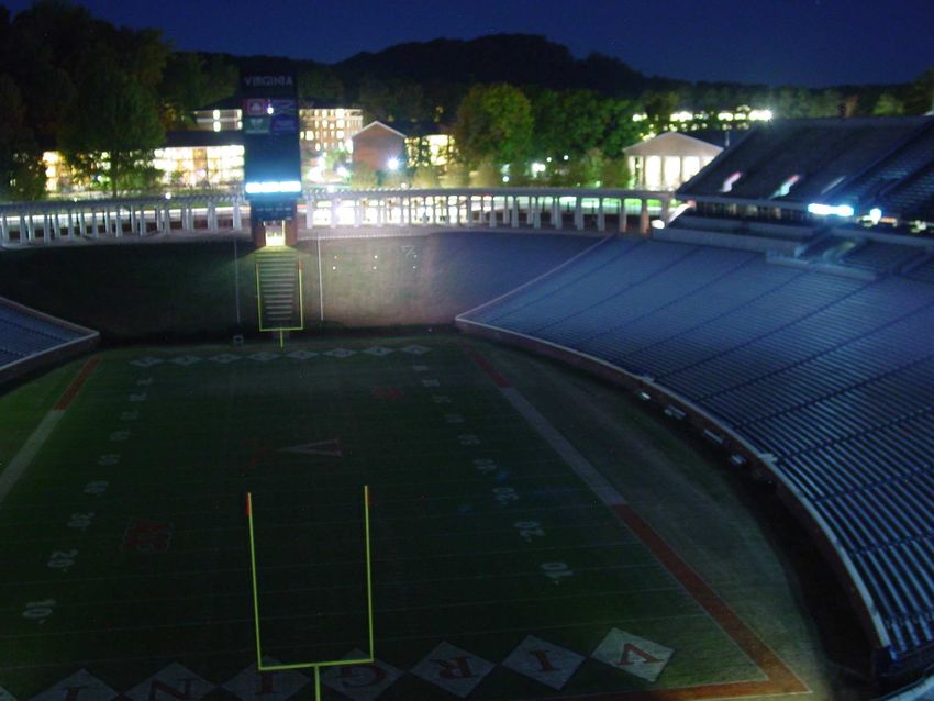
propose a novel framework for node localization in WSNs
that is very promising and allows for many future exten-
sions and more accurate results. We propose a constraint-
based label relaxation algorithm for mapping node IDs to
the locations, and four constraints (node, connectivity, time
and space), which are building blocks for very accurate and
very fast localization systems. We develop a sensor node
hardware prototype, called a SensorBall. We evaluate the
performance of a localization system for which we obtain
location accuracies of 2 − 5f t with a localization duration
ranging from 10 milliseconds to 2 minutes. We investigate              Figure 1: Stars, Planets or Smart Dust?
the range of a system built on our framework by consider-
ing realities of physical phenomena that occurs during light
propagation through the atmosphere.                              sized by several studies [14] [15] [16]. To address these chal-
   The rest of the paper is structured as follows. Section 2     lenges, and others (hardware cost, the energy expenditure,
is an overview of the state of art. The design of the Star-      the form factor, the small range, localization time), several
Dust framework is presented in Section 3. One implemen-          range-free localization schemes have been proposed. Sensor
tation and its performance evaluation are in Sections 4 and      nodes use primarily connectivity information for inferring
5, followed by a suite of system optimization techniques, in     proximity to a set of anchors. In the Centroid localization
Section 6. In Section 7 we present our conclusions.              scheme [17], a sensor node localizes to the centroid of its
                                                                 proximate beacon nodes. In APIT [18] each node decides
2.   RELATED WORK                                                its position based on the possibility of being inside or out-
                                                                 side of a triangle formed by any three beacons within node’s
   We present the prior work in localization in two major
                                                                 communication range. The Gradient algorithm [19], lever-
categories: the range-based, and the range-free schemes.
                                                                 ages the knowledge about the network density to infer the
   The range-based localization techniques have been de-
                                                                 average one hop length. This, in turn, can be transformed
signed to use either more expensive hardware (and hence
                                                                 into distances to nodes with known locations. DV-Hop [20]
higher accuracy) or just the radio transceiver. Ranging tech-
                                                                 uses the hop by hop propagation capability of the network
niques dependent on hardware are the time-of-flight (ToF)
                                                                 to forward distances to landmarks. More recently, several
and the time-difference-of-arrival (TDoA). Solutions that
                                                                 localization schemes that exploit the sensing capabilities of
use the radio are based on the received signal strength indi-
                                                                 sensor nodes, have been proposed. Spotlight [21] creates well
cator (RSSI) and more recently on radio interferometry.
                                                                 controlled (in time and space) events in the network while
   The ToF localization technique that is most widely used is
                                                                 the sensor nodes detect and timestamp this events. From
the GPS. GPS is a costly solution for a high accuracy local-
                                                                 the spatio-temporal knowledge for the created events and
ization of a large scale sensor network. AHLoS [6] employs
                                                                 the temporal information provided by sensor nodes, nodes’
a TDoA ranging technique that requires extensive hardware
                                                                 spatial information can be obtained. In a similar manner,
and solves relatively large nonlinear systems of equations.
                                                                 the Lighthouse system [22] uses a parallel light beam, that
The Cricket location-support system (TDoA) [7] can achieve
                                                                 is emitted by an anchor which rotates with a certain period.
a location granularity of tens of inches with highly direc-
                                                                 A sensor node detects the light beam for a period of time,
tional and short range ultrasound transceivers. In [2] the
                                                                 which is dependent on the distance between it and the light
location of a sniper is determined in an urban terrain, by
                                                                 emitting device.
using the TDoA between an acoustic wave and a radio bea-
                                                                    Many of the above localization solutions target specific
con. The PushPin project [8] uses the TDoA between ul-
                                                                 sets of requirements and are useful for specific applications.
trasound pulses and light flashes for node localization. The
                                                                 StarDust differs in that it addresses a particular demanding
RADAR system [9] uses the RSSI to build a map of signal
                                                                 set of requirements that are not yet solved well. StarDust is
strengths as emitted by a set of beacon nodes. A mobile
                                                                 meant for localizing air dropped nodes where node passive-
node is located by the best match, in the signal strength
                                                                 ness, high accuracy, low cost, small form factor and rapid lo-
space, with a previously acquired signature. In MAL [10],
                                                                 calization are all required. Many military applications have
a mobile node assists in measuring the distances (acting as
                                                                 such requirements.
constraints) between nodes until a rigid graph is generated.
The localization problem is formulated as an on-line state es-
timation in a nonlinear dynamic system [11]. A cooperative       3.   STARDUST SYSTEM DESIGN
ranging that attempts to achieve a global positioning from          The design of the StarDust system (and its name) was
distributed local optimizations is proposed in [12]. A very      inspired by the similarity between a deployed sensor net-
recent, remarkable, localization technique is based on radio     work, in which sensor nodes indicate their presence by emit-
interferometry, RIPS [13], which utilizes two transmitters to    ting light, and the Universe consisting of luminous and il-
create an interfering signal. The frequencies of the emitters    luminated objects: stars, galaxies, planets, etc. We depict
are very close to each other, thus the interfering signal will   this similarity in Figure 1, which shows the duality between
have a low frequency envelope that can be easily measured.       stars, galaxies and sensor nodes equipped with light emitting
The ranging technique performs very well. The long time          capabilities.
required for localization and multi-path environments pose          The main difficulty when applying the above ideas to the
significant challenges.                                          real world is the complexity of the hardware that needs to
   Real environments create additional challenges for the        be put on a sensor node so that the emitted light can be
range based localization schemes. These have been empha-         detected from thousands of feet. The energy expenditure for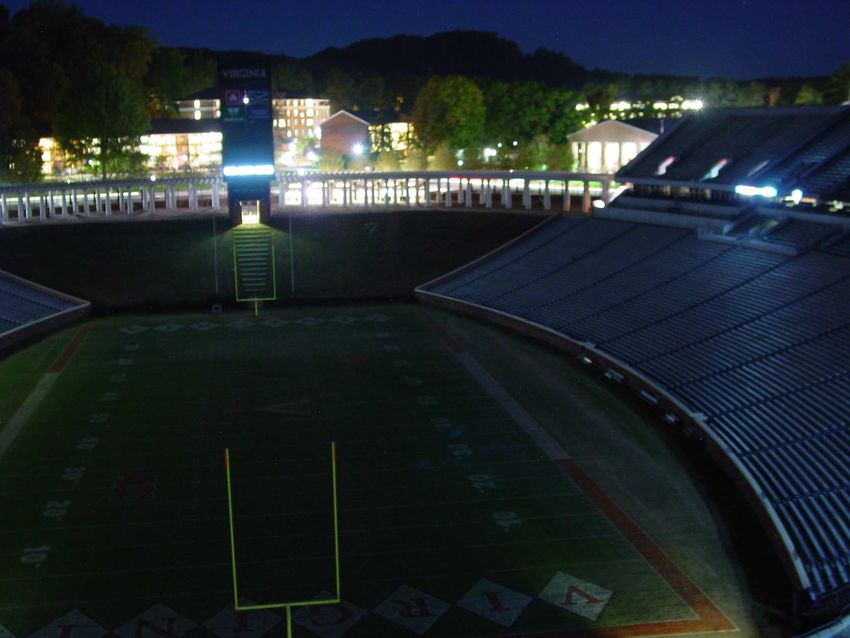
! "
#$
#$
(a) (b)
Figure 2: Corner-Cube Retroreflector (a) and an Figure 3: The StarDust system architecture
array of CCRs molded in plastic (b)
by using the color of a retro-reflected light, if a sensor
producing an intense enough light beam is also prohibitive. node has a unique color; b) by requiring sensor nodes
Instead, what we propose to use for sensor node local- to establish neighborhood information and report it
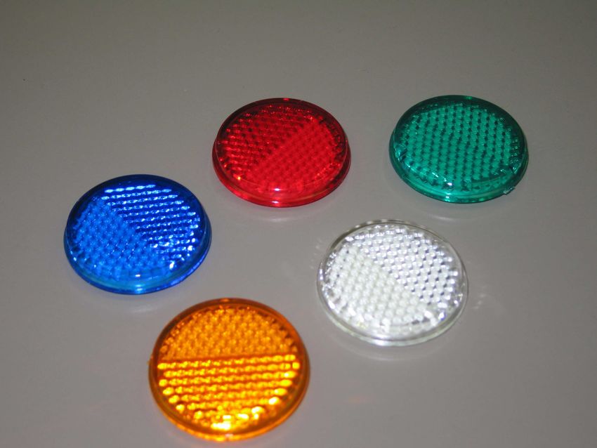
ization is a passive optical element called a retro-reflector. to a base station; c) by controlling the time sequence
The most common retro-reflective optical component is a of sensor nodes deployment and recording additional
Corner-Cube Retroreflector (CCR), shown in Figure 2(a). images; d) by controlling the location where a sensor
It consists of three mutually perpendicular mirrors. The node is deployed.
interesting property of this optical component is that an in-
coming beam of light is reflected back, towards the source • The computed locations are disseminated to the sensor
of the light, irrespective of the angle of incidence. This is network.
in contrast with a mirror, which needs to be precisely posi- The architecture of the StarDust system is shown in Fig-
tioned to be perpendicular to the incident light. A very com- ure 3. The architecture consists of two main components:
mon and inexpensive implementation of an array of CCRs is the first is centralized and it is located on a more power-
the retro-reflective plastic material used on cars and bicycles ful device. The second is distributed and it resides on all
for night time detection, shown in Figure 2(b). sensor nodes. The Central Device consists of the following:
In the StarDust system, each node is equipped with a the Light Emitter, the Image Processing module, the Node
small (e.g. 0.5in2 ) array of CCRs and the enclosure has ID Mapping module and the Radio Model. The distrib-
self-righting capabilities that orient the array of CCRs pre- uted component of the architecture is the Transfer Function,
dominantly upwards. It is critical to understand that the which acts as a filter for the incoming light. The aforemen-
upward orientation does not need to be exact. Even when tioned modules are briefly described below:
large angular variations from a perfectly upward orientation
are present, a CCR will return the light in the exact same • Light Emitter - It is a strobe light, capable of produc-
direction from which it came. ing very intense, collimated light pulses. The emitted
In the remaining part of the section, we present the archi- light is non-monochromatic (unlike a laser) and it is
tecture of the StarDust system and the design of its main characterized by a spectral density Ψ(λ), a function of
components. the wavelength. The emitted light is incident on the
CCRs present on sensor nodes.
3.1 System Architecture
The envisioned sensor network localization scenario is as • Transfer Function Φ(Ψ(λ)) - This is a bandpass filter
follows: for the incident light on the CCR. The filter allows a
portion of the original spectrum, to be retro-reflected.
• The sensor nodes are released, possibly in a controlled From here on, we will refer to the transfer function as
manner, from an aerial vehicle during the night. the color of a sensor node.
• The aerial vehicle hovers over the deployment area and • Image Processing - The Image Processing module ac-
uses a strobe light to illuminate it. The sensor nodes, quires high resolution images. From these images the
equipped with CCRs and optical filters (acting as col- locations and the colors of sensor nodes are obtained.
oring devices) have self-righting capabilities and retro- If only one set of pictures can be taken (i.e., one loca-
reflect the incoming strobe light. The retro-reflected tion of the light emitter/image analysis device), then
light is either ”white”, as the originating source light, the map of the field is assumed to be known as well
or colored, due to optical filters. as the distance between the imaging device and the
field. The aforementioned assumptions (field map and
• The aerial vehicle records a sequence of two images distance to it) are not necessary if the images can be
very close in time (msec level). One image is taken simultaneously taken from different locations. It is im-
when the strobe light is on, the other when the strobe portant to remark here that the identity of a node
light is off. The acquired images are used for obtaining can not be directly obtained through Image Process-
the locations of sensor nodes (which appear as lumi- ing alone, unless a specific characteristic of a sensor
nous spots in the image). node can be identified in the image.
• The aerial vehicle executes the mapping of node IDs to • Node ID Matching - This module uses the detected lo-
the identified locations in one of the following ways: a) cations and through additional techniques (e.g., sensor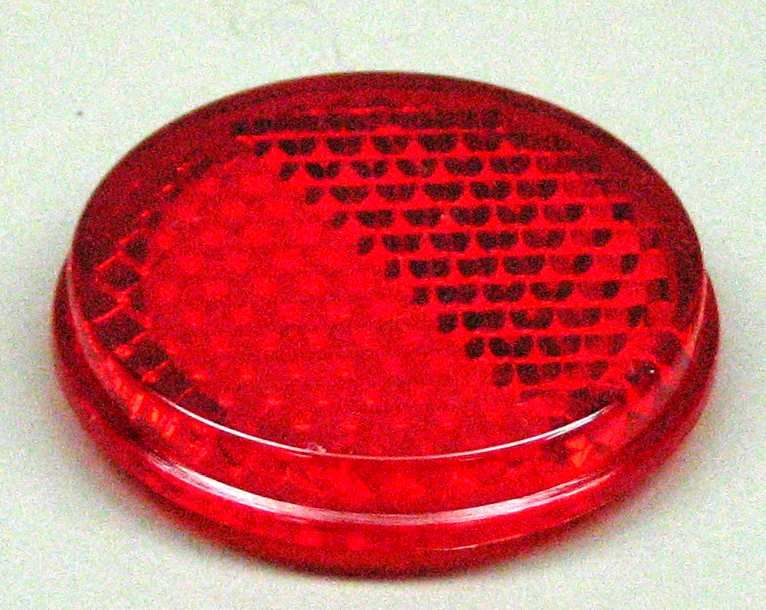
Algorithm 1 Image Processing
1: Background filtering
2: Retro-reflected light recognition through intensity filter-
   ing
3: Edge detection to obtain the location of sensor nodes
4: Color identification for each detected sensor node

      node coloring and connectivity information (G(Λ, E))
      from the deployed network) to uniquely identify the                     Figure 4: Probabilistic label relaxation
      sensor nodes observed in the image. The connectiv-
      ity information is represented by neighbor tables sent
      from each sensor node to the Central Device.                    and used to create Pref lect . This step is eased by the fact
   • Radio Model - This component provides an estimate                that the reflecting nodes should appear much brighter than
     of the radio range to the Node ID Matching module. It            any other illuminated object in the picture.
     is only used by node ID matching techniques that are               The third step runs an edge detection algorithm on Pref lect
     based on the radio connectivity in the network. The es-          to identify the boundary of the nodes present. A tool such as
     timate of the radio range R is based on the sensor node          Matlab provides a number of edge detection techniques. We
     density (obtained through the Image Processing mod-              used the bwboundaries function. For the obtained edges, the
     ule) and the connectivity information (i.e., G(Λ, E)).           location (x, y) (in the image) of each node is determined by
                                                                      computing the centroid of the points constituting its edges.
  The two main components of the StarDust architecture                Standard computer graphics techniques [23] are then used
are the Image Processing and the Node ID Mapping. Their               to transform the 2D locations of sensor nodes detected in
design and analysis is presented in the sections that follow.         multiple images into 3D sensor node locations. The color
                                                                      of the node is obtained as the color of the pixel located at
3.2    Image Processing                                               (x, y) in Plight .
   The goal of the Image Processing Algorithm (IPA) is to
identify the location of the nodes and their color. Note that         3.3    Node ID Matching
IPA does not identify which node fell where, but only what               The goal of the Node ID Matching module is to obtain
is the set of locations where the nodes fell.                         the identity (node ID) of a luminous spot in the image,
   IPA is executed after an aerial vehicle records two pic-           detected to be a sensor node. For this, we define V =
tures: one in which the field of deployment is illuminated            {(x1 , y1 ), (x2 , y2 ), ..., (xm , ym )} to be the set of locations of
and one when no illuminations is present. Let Pdark be the            the sensor nodes, as detected by the Image Processing mod-
picture of the deployment area, taken when no light was               ule and Λ = {λ1 , λ2 , ..., λm } to be the set of unique node IDs
emitted and Plight be the picture of the same deployment              assigned to the m sensor nodes, before deployment. From
area when a strong light beam was directed towards the                here on, we refer to node IDs as labels.
sensor nodes.                                                            We model the problem of finding the label λj of a node ni
   The proposed IPA has several steps, as shown in Algo-              as a probabilistic label relaxation problem, frequently used
rithm 1. The first step is to obtain a third picture Pf ilter         in image processing/understanding. In the image process-
where only the differences between Pdark and Plight remain.           ing domain, scene labeling (i.e., identifying objects in an
Let us assume that Pdark has a resolution of n × m, where             image) plays a major role. The goal of scene labeling is to
n is the number of pixels in a row of the picture, while m is         assign a label to each object detected in an image, such that
the number of pixels in a column of the picture. Then Pdark           an appropriate image interpretation is achieved. It is pro-
is composed of n × m pixels noted Pdark (i, j), i ∈ 1 ≤ i ≤           hibitively expensive to consider the interactions among all
n, 1 ≤ j ≤ m. Similarly Plight is composed of n × m pixels            the objects in an image. Instead, constraints placed among
noted Plight (i, j), 1 ≤ i ≤ n, 1 ≤ j ≤ m.                            nearby objects generate local consistencies and through it-
   Each pixel P is described by an RGB value where the R              eration, global consistencies can be obtained.
value is denoted by P R , the G value is denoted by P G , and            The main idea of the sensor node localization through
the B value is denoted by P B . IPA then generates the third          probabilistic label relaxation is to iteratively compute the
picture, Pf ilter , through the following transformations:            probability of each label being the correct label for a sensor
                                                                      node, by taking into account, at each iteration, the ”sup-
            PfRilter (i, j) = Plight
                                R              R
                                     (i, j) − Pdark (i, j)            port” for a label. The support for a label can be understood
              G                 G              G
                                                               (1)    as a hint or proof, that a particular label is more likely to
            Pf ilter (i, j) = Plight (i, j) − Pdark (i, j)
                                                                      be the correct one, when compared with the other potential
            PfBilter (i, j) = Plight
                                B              B
                                     (i, j) − Pdark (i, j)
                                                                      labels for a sensor node. We pictorially depict this main
   After this transformation, all the features that appeared          idea in Figure 4. As shown, node ni has a set of candidate
in both Pdark and Plight are removed from Pf ilter . This             labels {λ1 , ..., λk }. Each of the labels has a different value
simplifies the recognition of light retro-reflected by sensor         for the Support function Q(λk ). We defer the explanation of
nodes.                                                                how the Support function is implemented until the subsec-
   The second step consists of identifying the elements con-          tions that follow, where we provide four concrete techniques.
tained in Pf ilter that retro-reflect light. For this, an intensity   Formally, the algorithm is outlined in Algorithm 2, where
filter is applied to Pf ilter . First IPA converts Pf ilter into a    the equations necessary for computing the new probability
grayscale picture. Then the brightest pixels are identified           Pni (λk ) for a label λk of a node ni , are expressed by the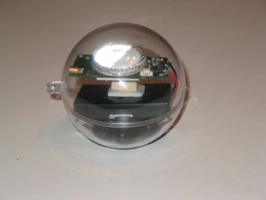
Algorithm 2 Label Relaxation                                              As a result, the label relaxation algorithm (Algorithm 2)
 1: for each sensor node ni do                                         consists of the following steps: one label is assigned to each
 2:   assign equal prob. to all possible labels                        sensor node (lines 1-3 of the algorithm), implicitly having
 3: end for                                                            a probability Pni (λk ) = 1 ; the algorithm executes a single
 4: repeat                                                             iteration, when the support function, simply, reiterates the
 5:   converged ← true                                                 confidence in the unique labeling.
 6:   for each sensor node ni do                                          However, it is often the case that unique colors for each
 7:      for each each label λj of ni do                               node will not be available. It is interesting to discuss here
 8:        compute the Support label λj : Equation 4                   the influence that the size of the coloring space (i.e., |C|)
 9:      end for                                                       has on the accuracy of the localization algorithm. Several
10:      compute K for the node ni : Equation 3                        cases are discussed below:
11:      for each each label λj do
12:        update probability of label λj : Equation 2                    • If |C| = 0, no colors are used and the sensor nodes are
13:        if |new prob. − old prob.| ≥ ² then                              equipped with simple CCRs that reflect back all the
14:           converged ← f alse                                            incoming light (i.e., no filtering, and no coloring of the
15:        end if                                                           incoming light). From the image processing system,
16:      end for                                                            the position of sensor nodes can still be obtained. Since
17:   end for                                                               all nodes appear white, no single sensor node can be
18: until converged = true                                                  uniquely identified.

                                                                          • If |C| = m − 1 then there are enough unique colors for
                                                                            all nodes (one node remains white, i.e. no coloring),
following equations:
                                                                            the problem is trivially solved. Each node can be iden-
                                                                            tified, based on its unique color. This is the scenario
                                1                                           for the relaxation with color constraints.
               Pns+1 (λk ) =      Pns (λk )Qsni (λk )           (2)
                  i
                               Kni i
                                                                          • If |C| ≥ 1, there are several options for how to parti-
where Kni is a normalizing constant, given by:
                                                                            tion the coloring space. If C = {c1 } one possibility is
                             X
                             N                                              to assign the color c1 to a single node, and leave the
                     Kni =         Pnsi (λk )Qsni (λk )         (3)         remaining m − 1 sensor nodes white, or to assign the
                             k=1                                            color c1 to more than one sensor node. One can ob-
and Qsni (λk ) is:                                                          serve that once a color is assigned uniquely to a sensor
                                                                            node, in effect, that sensor node is given the status of
        Qsni (λk ) = “support for label λk of node ni ”         (4)         “anchor”, or node with known location.
   The label relaxation algorithm is iterative and it is poly-
                                                                          It is interesting to observe that there is an entire spec-
nomial in the size of the network(number of nodes). The
                                                                       trum of possibilities for how to partition the set of sensor
pseudo-code is shown in Algorithm 2. It initializes the prob-
                                                                       nodes in equivalence classes (where an equivalence class is
abilities associated with each possible label, for a node ni ,
                                                                       represented by one color), in order to maximize the success
through a uniform distribution. At each iteration s, the al-
                                                                       of the localization algorithm. One of the goals of this paper
gorithm updates the probability associated with each label,
                                                                       is to understand how the size of the coloring space and its
by considering the Support Qsni (λk ) for each candidate label
                                                                       partitioning affect localization accuracy.
of a sensor node.
                                                                          Despite the simplicity of this method of constraining the
   In the sections that follow, we describe four different tech-
                                                                       set of labels that can be assigned to a node, we will show
niques for implementing the Support function: based on
                                                                       that this technique is very powerful, when combined with
node coloring, radio connectivity, the time of deployment
                                                                       other relaxation techniques.
(time) and the location of deployment (space). While some
of these techniques are simplistic, they are primitives which,         3.3.2    Relaxation with Connectivity Constraints
when combined, can create powerful localization systems.
                                                                          Connectivity information, obtained from the sensor net-
These design techniques have different trade-offs, which we
                                                                       work through beaconing, can provide additional information
will present in Section 3.3.6.
                                                                       for locating sensor nodes. In order to gather connectivity in-
3.3.1     Relaxation with Color Constraints                            formation, the following need to occur: 1) after deployment,
                                                                       through beaconing of HELLO messages, sensor nodes build
   The unique mapping between a sensor node’s position
                                                                       their neighborhood tables; 2) each node sends its neighbor
(identified by the image processing) and a label can be ob-
                                                                       table information to the Central device via a base station.
tained by assigning a unique color to each sensor node. For
                                                                          First, let us define G = (Λ, E) to be the weighted connec-
this we define C = {c1 , c2 , ..., cn } to be the set of unique col-
                                                                       tivity graph built by the Central device from the received
ors available and M : Λ → C to be a one-to-one mapping of
                                                                       neighbor table information. In G the edge (λi , λj ) has a
labels to colors. This mapping is known prior to the sensor
                                                                       weight gij represented by the number of beacons sent by λj
node deployment (from node manufacturing).
                                                                       and received by λi . In addition, let R be the radio range of
   In the case of color constrained label relaxation, the sup-
                                                                       the sensor nodes.
port for label λk is expressed as follows:
                                                                          The main idea of the connectivity constrained label re-
                                                                       laxation is depicted in Figure 5 in which two nodes ni and
                             Qsni (λk ) = 1                     (5)    nj have been assigned all possible labels. The confidence in
Algorithm 3 Localization
1: Estimate the radio range R
2: Execute the Label Relaxation Algorithm with Support
Function given by Equation 6 for neighbors less than R
apart
3: for each sensor node ni do
4: node identity is λk with max. prob.
5: end for
√
(the expected k = 8N ); if 2u ≤ R ≤ 5u √ each node has
Figure 5: Label relaxation with connectivity con- twelve neighbors ( the expected k = 12N ); if 5u ≤ R ≤ 3u
straints each node has twenty neighbors (the expected k = 20N )
For a given t = k/4N we take R to be the middle √ of the
interval. As an example, if t = 5 then R = (3 + 5)u/2.
each of the candidate labels for a sensor node, is represented A quadratic fitting for R over the possible values of t, pro-
by a probability, shown in a dotted rectangle. duces the following closed-form solution for the communi-
It is important to remark that through beaconing and the cation range R, as a function of network connectivity k,
reporting of neighbor tables to the Central Device, a global assuming L and N constant:
view of all constraints in the network can be obtained. It is
critical to observe that these constraints are among labels. " 2 #
As shown in Figure 5 two constraints exist between nodes ni L k k
R(k) = √ −0.051 + 0.66 + 0.6 (7)
and nj . The constraints are depicted by gi2,j2 and gi2,jM , N 4N 4N
the number of beacons sent the labels λj2 and λjM and
received by the label λi2 . We investigate the accuracy of our model in Section 5.2.1.
The support for the label λk of sensor node ni , resulting 3.3.3 Relaxation with Time Constraints
from the “interaction” (i.e., within radio range) with sensor
node nj is given by: Time constraints can be treated similarly with color con-
straints. The unique identification of a sensor node can be
obtained by deploying sensor nodes individually, one by one,
X
M
and recording a sequence of images. The sensor node that
Qsni (λk ) = gλk λm Pnsj (λm ) (6) is identified as new in the last picture (it was not identi-
m=1
fied in the picture before last) must be the last sensor node
As a result, the localization algorithm (Algorithm 3 con- dropped.
sists of the following steps: all labels are assigned to each In a similar manner with color constrained label relax-
sensor node (lines 1-3 of the algorithm), and implicitly each ation, the time constrained approach is very simple, but
label has a probability initialized to Pni (λk ) = 1/|Λ|; in each may take too long, especially for large scale systems. While
iteration, the probabilities for the labels of a sensor node are it can be used in practice, it is unlikely that only a time con-
updated, when considering the interaction with the labels of strained label relaxation is used. As we will see, by combin-
sensor nodes within R. It is important to remark that the ing constrained-based primitives, realistic localization sys-
identity of the nodes within R is not known, only the candi- tems can be implemented.
date labels and their probabilities. The relaxation algorithm The support function for the label relaxation with time
converges when, during an iteration, the probability of no constraints is defined identically with the color constrained
label is updated by more than ². relaxation:
The label relaxation algorithm based on connectivity con-
straints, enforces such constraints between pairs of sensor
Qsni (λk ) = 1 (8)
nodes. For a large scale sensor network deployment, it is
not feasible to consider all pairs of sensor nodes in the net- The localization algorithm (Algorithm 2 consists of the
work. Hence, the algorithm should only consider pairs of following steps: one label is assigned to each sensor node
sensor nodes that are within a reasonable communication (lines 1-3 of the algorithm), and implicitly having a proba-
range (R). We assume a circular radio range and a sym- bility Pni (λk ) = 1 ; the algorithm executes a single iteration,
metric connectivity. In the remaining part of the section we when the support function, simply, reiterates the confidence
propose a simple analytical model that estimates the radio in the unique labeling.
range R for medium-connected networks (less than 20 neigh-
bors per R). We consider the following to be known: the size 3.3.4 Relaxation with Space Constraints
of the deployment field (L), the number of sensor nodes de- Spatial information related to sensor deployment can also
ployed (N ) and the total number of unidirectional (i.e., not be employed as another input to the label relaxation al-
symmetric) one-hop radio connections in the network (k). gorithm. To do that, we use two types of locations: the
For our analysis, we uniformly distribute the sensor nodes node location pn and the label location pl . The former
in √
a square area of length L, by using a grid √ of unit length pn is defined as the position of nodes (xn , yn , zn ) after de-
L/ N . We use the substitution u = L/ N to simplify ployment, which can be obtained through Image Processing
the notation,
√ in order to distinguish the following cases: if as mentioned in Section 3.3. The latter pl is defined as
u ≤ R ≤ 2u √ each node has four neighbors (the expected the location (xl , yl , zl ) where a node is dropped. We use
k = 4N ); if 2u ≤ R ≤ 2u each node has eight neighbors Dλnm
i
to denote the horizontal distance between the location1.4
σ = 0.5
σ=1
1.2 σ=2
Node Density
1
1
0.8 0.8
PDF
0.6
0.6 0.4
0.2
0.4 0
4
3
0.2 2
1
-4 0
-3
-2 -1 Y
0 -1
0
1
-2
-3
0 1 2 3 4 5 6 7 8 X 2
3
4 -4
Distance D
Figure 7: Probability distribu- Figure 8: Distribution of nodes
Figure 6: Relaxation with space
tion of distances
constraints
of the label
p λm and the location of the node ni . Clearly,
Dλnmi
= (xn − xl )2 + (yn − yl )2 .
At the time of a sensor node release, the one-to-one map-
ping between the node and its label is known. In other
words, the label location is the same as the node location
at the release time. After release, the label location infor-
mation is partially lost due to the random factors such as
wind and surface impact. However, statistically, the node
locations are correlated with label locations. Such correla-
tion depends on the airdrop methods employed and envi- (a) (b)
ronments. For the sake of simplicity, let’s assume nodes are
dropped from the air through a helicopter hovering in the
air. Wind can be decomposed into three components X, ~ Y~ Figure 9: A step through the algorithm. After ini-
and Z.~ Only X ~ and Y~ affect the horizontal distance a node tialization (a) and after the 1st iteration for node ni
can travel. According to [24], we can assume that X ~ and Y~ (b)
follow an independent normal distribution. Therefore, the
absolute value of the wind speed follows a Rayleigh distrib-
ution. Obviously the higher the wind speed is, the further a indicates that we can not use the spatial-based relaxation
node would land away horizontally from the label location. to recursively narrow down the potential labels for a node.
If we assume that the distance D is a function of the wind Second, if nodes are released at different locations that are
speed V [25] [26], we can obtain the probability distribution far away from each other, we have: (i) If node ni has label
of D under a given wind speed distribution. Without loss λk , Pnsi (λk ) → 1 when s → ∞, (ii) If node ni does not have
of generality, we assume that D is proportional to the wind label λk , Pnsi (λk ) → 0 when s → ∞. In this second scenario,
speed. Therefore, D follows the Rayleigh distribution as there are multiple labels (one label per release), hence it
well. As shown in Figure 6, the spatial-based relaxation is a is possible to correlate release times (labels) with positions
recursive process to assign the probability that a nodes has on the ground. These results indicate that spatial-based
a certain label by using the distances between the location relaxation can label the node with a very high probability if
of a node with multiple label locations. the physical separation among nodes is large.
We note that the distribution of distance D affects the 3.3.5 Relaxation with Color and Connectivity Con-
probability with which a label is assigned. It is not nec- straints
essarily true that the nearest label is always chosen. For
example, if D follows the Rayleigh(σ 2 ) distribution, we can One of the most interesting features of the StarDust archi-
obtain the Probability Density Function (PDF) of distances tecture is that it allows for hybrid localization solutions to be
as shown in Figure 7. This figure indicates that the possi- built, depending on the system requirements. One example
bility of a node to fall vertically is very small under windy is a localization system that uses the color and connectivity
conditions (σ > 0), and that the distance D is affected by constraints. In this scheme, the color constraints are used
the σ. The spatial distribution of nodes for σ = 1 is shown for reducing the number of candidate labels for sensor nodes,
in Figure 8. Strong wind with a high σ value leads to a to a more manageable value. As a reminder, in the connec-
larger node dispersion. More formally, given a probability tivity constrained relaxation, all labels are candidate labels
density function P DF (D), the support for label λk of sensor for each sensor node. The color constraints are used in the
node ni can be formulated as: initialization phase of Algorithm 3 (lines 1-3). After the ini-
tialization, the standard connectivity constrained relaxation
algorithm is used.
Qsni (λk ) = P DF (Dλnki ) (9) For a better understanding of how the label relaxation
It is interesting to point out two special cases. First, if algorithm works, we give a concrete example, exemplified
all nodes are released at once (i.e., only one label location in Figure 9. In part (a) of the figure we depict the data
for all released nodes), the distance D from a node to all structures associated with nodes ni and nj after the ini-
labels is the same. In this case, Pns+1
i
(λk ) = Pnsi (λk ), which tialization steps of the algorithm (lines 1-6), as well as thenumber of beacons between different labels (as reported by
the network, through G(Λ, E)). As seen, the potential labels
(shown inside the vertical rectangles) are assigned to each
node. Node ni can be any of the following: 11, 8, 4, 1. Also
depicted in the figure are the probabilities associated with
each of the labels. After initialization, all probabilities are
equal.
Part (b) of Figure 9 shows the result of the first iteration
of the localization algorithm for node ni , assuming that node (a) (b)
nj is the first wi chosen in line 7 of Algorithm 3. By using
Equation 6, the algorithm computes the ”support” Q(λi )
for each of the possible labels for node ni . Once the Q(λi )’s Figure 10: SensorBall with self-righting capabilities
are computed, the normalizing constant, given by Equation (a) and colored CCRs (b)
3 can be obtained. The last step of the iteration is to update
the probabilities associated with all potential labels of node
ni , as given by Equation 2.
One interesting problem, which we explore in the perfor- The StarDust localization framework, depicted in Figure
mance evaluation section, is to assess the impact the parti- 3, is flexible in that it enables the development of new lo-
tioning of the color set C has on the accuracy of localization. calization systems, based on the four proposed label relax-
When the size of the coloring set is smaller than the number ation schemes, or the inclusion of other, yet to be invented,
of sensor nodes (as it is the case for our hybrid connectiv- schemes. For our performance evaluation we implemented
ity/color constrained relaxation), the system designer has a version of the StarDust framework, namely the one pro-
the option of allowing one node to uniquely have a color posed in Section 3.3.5, where the constraints are based on
(acting as an anchor), or multiple nodes. Intuitively, by as- color and connectivity.
signing one color to more than one node, more constraints The Central device of the StarDust system consists of the
(distributed) can be enforced. following: the Light Emitter - we used a common-off-the-
shelf flash light (QBeam, 3 million candlepower); the im-
3.3.6 Relaxation Techniques Analysis age acquisition was done with a 3 megapixel digital cam-
The proposed label relaxation techniques have different era (Sony DSC-S50) which provided the input to the Image
trade-offs. For our analysis of the trade-offs, we consider Processing algorithm, implemented in Matlab.
the following metrics of interest: the localization time (du- For sensor nodes we built a custom sensor node, called
ration), the energy consumed (overhead), the network size SensorBall, with self-righting capabilities, shown in Figure
(scale) that can be handled by the technique and the local- 10(a). The self-righting capabilities are necessary in order to
ization accuracy. The parameters of interest are the follow- orient the CCR predominantly upwards. The CCRs that we
ing: the number of sensor nodes (N ), the energy spent for used were inexpensive, plastic molded, night time warning
one aerial drop (²d ), the energy spent in the network for col- signs commonly available on bicycles, as shown in Figure
lecting and reporting neighbor information ²b and the time 10(b). We remark here the low quality of the CCRs we
Td taken by a sensor node to reach the ground after being used. The reflectivity of each CCR (there are tens molded
aerially deployed. The cost comparison of the different label in the plastic container) is extremely low, and each CCR
relaxation techniques is shown in the table below. is not built with mirrors. A reflective effect is achieved by
employing finely polished plastic surfaces. We had 5 colors
Criteria Color Connectivity Time Space available, in addition to the standard CCR, which reflects
all the incoming light (white CCR). For a slightly higher
Duration 0 N Tb N Td 0
price (ours were 20cents/piece), better quality CCRs can be
Overhead ²d ²d + N ²b N ²d ²d
employed. Higher quality (better mirrors) would translate
Scale |C| |N | |N | |N |
in more accurate image processing (better sensor node de-
Accuracy High Low High Medium tection) and smaller form factor for the optical component
(an array of CCRs with a smaller area can be used).
Table 1: Comparison of label relaxation techniques
The sensor node platform we used was the micaZ mote.
The code that runs on each node is a simple application
As shown, the relaxation techniques based on color and which broadcasts 100 beacons, and maintains a neighbor
space constraints have the lowest localization duration, zero, table containing the percentage of successfully received bea-
for all practical purposes. The scalability of the color based cons, for each neighbor. On demand, the neighbor table is
relaxation technique is, however, limited to the number of reported to a base station, where the node ID mapping is
unique color filters that can be built. The narrower the performed.
Transfer Function Ψ(λ), the larger the number of unique col-
ors that can be created. The manufacturing costs, however,
are increasing as well. The scalability issue is addressed by 5. SYSTEM EVALUATION
all other label relaxation techniques. Most notably, the time In this section we present the performance evaluation of a
constrained relaxation, which is very similar to the color- system implementation of the StarDust localization frame-
constrained relaxation, addresses the scale issue, at a higher work. The three major research questions that our eval-
deployment cost. uation tries to answer are: the feasibility of the proposed
framework (can sensor nodes be optically detected at large
4. SYSTEM IMPLEMENTATION distances), the localization accuracy of one actual imple-Figure 11: The field in the dark Figure 12: The illuminated field
Figure 13: The difference: Figure 11 - Fig- Figure 14: Retroreflectors detected in Fig-
ure 12 ure 13
mentation of the StarDust framework, and whether or not inches above ground. From here on, we will refer to these two
atmospheric conditions can affect the recognition of sen- experimental set-ups as the low connectivity and the high
sor nodes in an image. The first two questions are in- connectivity networks, respectively because when nodes are
vestigated by evaluating the two main components of the on the ground the communication range is low resulting in
StarDust framework: the Image Processing and the Node less neighbors than when the nodes are elevated and have a
ID Matching. These components have been evaluated sep- greater communication range. The metrics of interest are:
arately mainly because of lack of adequate facilities. We the localization error (defined as the distance between the
wanted to evaluate the performance of the Image Process- computed location and the true location - known from the
ing Algorithm in a long range, realistic, experimental set-up, manual placement), the percentage of nodes correctly local-
while the Node ID Matching required a relatively large area, ized, the convergence of the label relaxation algorithm, the
available for long periods of time (for connectivity data gath- time to localize and the robustness of the node ID mapping
ering). The third research question is investigated through to errors in the Image Processing module.
a computer modeling of atmospheric phenomena. The parameters that we vary experimentally are: the an-
For the evaluation of the Image Processing module, we gle under which images are taken, the focus of the camera,
performed experiments in a football stadium where we de- and the degree of connectivity. The parameters that we
ploy 6 sensor nodes in a 3×2 grid. The distance between the vary in simulations (subsequent to image acquisition and
Central device and the sensor nodes is approximately 500f t. connectivity collection) the number of colors, the number
The metrics of interest are the number of false positives and of anchors, the number of false positives or negatives as in-
false negatives in the Image Processing Algorithm. put to the Node ID Matching component, the distance be-
For the evaluation of the Node ID Mapping component, tween the imaging device and sensor network (i.e., range),
we deploy 26 sensor nodes in an 120 × 60f t2 flat area of a atmospheric conditions (light attenuation coefficient) and
stadium. In order to investigate the influence the radio con- CCR reflectance (indicative of its quality).
nectivity has on localization accuracy, we vary the height
above ground of the deployed sensor nodes. Two set-ups 5.1 Image Processing
are used: one in which the sensor nodes are on the ground, For the IPA evaluation, we deploy 6 sensor nodes in a 3×2
and the second one, in which the sensor nodes are raised 3 grid. We take 13 sets of pictures using different orientations3 60
False Positives Connected
False Negatives 50 Not Connected
2
Count
40
Count
30
1
20
0 10
1 2 3 4 5 6 7 8 9 10 11
0
Experiment Number
0 10 20 30 40 50 60 70 80 90
Distance [feet]
Figure 15: False Positives and Negatives for the 6
sensor nodes Figure 16: The number of existing and missing radio
connections in the sparse connectivity experiment
70
of the camera and different zooming factors. All pictures Connected
were taken from the same location. Each set is composed of 60 Not Connected
a picture taken in the dark and of a picture taken with a light 50
beam pointed at the nodes. We process the pictures offline 40
Count
using a Matlab implementation of IPA. Since we are inter- 30
ested in the feasibility of identifying colored sensor nodes at
20
large distance, the end result of our IPA is the 2D location
10
of sensor nodes (position in the image). The transformation
to 3D coordinates can be done through standard computer 0
0 10 20 30 40 50 60 70 80 90 10 11 12
graphics techniques [23]. Distance [feet]
One set of pictures obtained as part of our experiment is
shown in Figures 11 and 12. The execution of our IPA algo-
rithm results in Figure 13 which filters out the background, Figure 17: The number of existing and missing radio
and Figure 14 which shows the output of the edge detection connections in the high connectivity experiment
step of IPA. The experimental results are depicted in Fig-
ure 15. For each set of pictures the graph shows the number
of false positives (the IPA determines that there is a node the coloring space available to us was 5 (5 colors). Through
while there is none), and the number of false negatives (the simulations of color assignment (not connectivity) we are
IPA determines that there is no node while there is one). able to investigate the influence that the size of the coloring
In about 45% of the cases, we obtained perfect results, i.e., space has on the accuracy of localization. The value of the
no false positives and no false negatives. In the remaining parameter ² used in Algorithm 2 was 0.001. The results pre-
cases, we obtained a number of false positives of at most sented here represent averages over the randomly generated
one, and a number of false negatives of at most two. colorings and over all experimental data sets.
We exclude two pairs of pictures from Figure 15. In the We first investigate the accuracy of our proposed Radio
first excluded pair, we obtain 42 false positives and in the Model, and subsequently use the derived values for the radio
second pair 10 false positives and 7 false negatives. By care- range in the evaluation of the Node ID matching component.
fully examining the pictures, we realized that the first pair
was taken out of focus and that a car temporarily appeared 5.2.1 Radio Model
in one of the pictures of the second pair. The anomaly in From experiments, we obtain the average number of ob-
the second set was due to the fact that we waited too long served beacons (k, defined in Section 3.3.2) for the low con-
to take the second picture. If the pictures had been taken a nectivity network of 180 beacons and for the high connectiv-
few milliseconds apart, the car would have been represented ity network of 420 beacons. From our Radio Model (Equa-
on either both or none of the pictures and the IPA would tion 7, we obtain a radio range R = 25f t for the low con-
have filtered it out. nectivity network and R = 40f t for the high connectivity
network.
5.2 Node ID Matching To estimate the accuracy of our simple model, we plot
We evaluate the Node ID Matching component of our sys- the number of radio links that exist in the networks, and the
tem by collecting empirical data (connectivity information) number of links that are missing, as functions of the distance
from the outdoor deployment of 26 nodes in the 120 × 60f t2 between nodes. The results are shown in Figures 16 and 17.
area. We collect 20 sets of data for the high connectivity We define the average radio range R to be the distance over
and low connectivity network deployments. Off-line we in- which less than 20% of potential radio links, are missing.
vestigate the influence of coloring on the metrics of interest, As shown in Figure 16, the radio range is between 20f t and
by randomly assigning colors to the sensor nodes. For one 25f t. For the higher connectivity network, the radio range
experimental data set we generate 50 random assignments was between 30f t and 40f t.
of colors to sensor nodes. It is important to observe that, We choose two conservative estimates of the radio range:
for the evaluation of the Node ID Matching algorithm (color 20f t for the low connectivity case and 35f t for the high
and connectivity constrained), we simulate the color assign- connectivity case, which are in good agreement with the
ment to sensor nodes. As mentioned in Section 4 the size of values predicted by our Radio Model.45
105 R=15feet
40
Localization Error [feet]
R=15feet
Convergence Rate [x100]
R=20feet
35 R=20feet R=25feet
30 R=25feet
100
25
20
15 95
10
5
0 90
0 5 10 15 20 0 5 10 15 20
Number of Colors Number of Colors
Figure 18: Localization error Figure 20: Convergence error
100 16
% Correct Localized [x100]
90 0 anchors
14
Localization Error [feet]
80 2 anchors
70 12
4 anchors
60 10 6 anchors
50 8 anchors
R=15feet 8
40
R=20feet
30 6
R=25feet
20 4
10
2
0
0 5 10 15 20 0
4 6 8
Number of Colors
Number of Colors
Figure 19: Percentage of nodes correctly localized Figure 21: Localization error vs. number of colors
5.2.2 Localization Error vs. Coloring Space Size we want to experimentally verify our intuition that assigning
In this experiment we investigate the effect of the number more nodes to a color can benefit the localization accuracy,
of colors on the localization accuracy. For this, we randomly by enforcing more constraints, as opposed to uniquely as-
assign colors from a pool of a given size, to the sensor nodes. signing a color to a single node.
We then execute the localization algorithm, which uses the For this, we fix the number of available colors to either 4,
empirical data. The algorithm is run for three different radio 6 or 8 and vary the number of nodes that are given unique
ranges: 15, 20 and 25f t, to investigate its influence on the colors, from 0, up to the maximum number of colors (4, 6
localization error. or 8). Naturally, if we have a maximum number of colors
The results are depicted in Figure 18 (localization error) of 4, we can assign at most 4 anchors. The experimental
and Figure 19 (percentage of nodes correctly localized). As results are depicted in Figure 21 (localization error) and
shown, for an estimate of 20f t for the radio range (as pre- Figure 22 (percentage of sensor node correctly localized).
dicted by our Radio Model) we obtain the smallest localiza- As expected, the localization accuracy increases with the
tion errors, as small as 2f t, when enough colors are used. increase in the number of colors available (larger coloring
Both Figures 18 and 19 confirm our intuition that a larger space). Also, for a given size of the coloring space (e.g.,
number of colors available significantly decrease the error in 6 colors available), if more colors are uniquely assigned to
localization. sensor nodes then the localization accuracy decreases. It is
The well known fact that relaxation algorithms do not al- interesting to observe that by assigning colors uniquely to
ways converge, was observed during our experiments. The nodes, the benefit of having additional colors is diminished.
percentage of successful runs (when the algorithm converged) Specifically, if 8 colors are available and all are assigned
is depicted in Figure 20. As shown, in several situations, uniquely, the system would be less accurately localized (error
the algorithm failed to converge (the algorithm execution ≈ 7f t), when compared to the case of 6 colors and no unique
was stopped after 100 iterations per node). If the algorithm assignments of colors (≈ 5f t localization error).
does not converge in a predetermined number of steps, it The same trend, of a less accurate localization can be
will terminate and the label with the highest probability observed in Figure 22, which shows the percentage of nodes
will provide the identity of the node. It is very probable that correctly localized (i.e., 0f t localization error). As shown, if
the chosen label is incorrect, since the probabilities of some we increase the number of colors that are uniquely assigned,
of labels are constantly changing (with each iteration).The the percentage of nodes correctly localized decreases.
convergence of relaxation based algorithms is a well known
issue. 5.2.4 Localization Error vs. Connectivity
We collected empirical data for two network deployments
5.2.3 Localization Error vs. Color Uniqueness with different degrees of connectivity (high and low) in or-
As mentioned in the Section 3.3.1, a unique color gives a der to assess the influence of connectivity on location ac-
sensor node the statute of an anchor. A sensor node that is curacy. The results obtained from running our localization
an anchor can unequivocally be identified through the Image algorithm are depicted in Figure 23 and Figure 24. We var-
Processing module. In this section we investigate the effect ied the number of colors available and assigned no anchors
unique colors have on the localization accuracy. Specifically, (i.e., no unique assignments of colors).140 100
% Correct Localized [x100]
0 anchors 90 Low Connectivity
% Correct Localized [x100]
120 2 anchors 80 High Connectivity
100 4 anchors 70
6 anchors 60
80 8 anchors 50
60 40
30
40
20
20 10
0
0 0 2 4 6 8 10 12
4 6 8
Number of Colors
Number of Colors
Figure 22: Percentage of nodes correctly localized Figure 24: Percentage of nodes correctly localized
vs. number of colors 14
12 4 colors
Localization Error [feet]
45 8 colors
10
Localization Error [feet]
40 12 colors
Low Connectivity
35 8
High Connectivity
30 6
25
4
20
15 2
10 0
5 0 4 8 12 16
0 % False Negatives [x100]
0 2 4 6 8 10 12
Number of Colors
Figure 25: Impact of false negatives on the localiza-
tion error
Figure 23: Localization error vs. number of colors
list of nodes detected by the Image Processing algorithm (we
In both scenarios, as expected, localization error decrease artificially introduced false negatives in the Image Process-
with an increase in the number of colors. It is interest- ing). The effect of false negatives on localization accuracy
ing to observe, however, that the low connectivity scenario is depicted in Figure 25. As seen in the figure if the number
improves the localization accuracy quicker, from the addi- of false negatives is 15%, the error in position estimation
tional number of colors available. When the number of col- doubles when 4 colors are available. It is interesting to ob-
ors becomes relatively large (twelve for our 26 sensor node serve that the scenario when more colors are available (e.g.,
network), both scenarios (low and high connectivity) have 12 colors) is being affected more drastically than the sce-
comparable localization errors, of less that 2f t. The same nario with less colors (e.g., 4 colors). The benefit of having
trend of more accurate location information is evidenced by more colors available is still being maintained, at least for
Figure 24 which shows that the percentage of nodes that the range of colors we investigated (4 through 12 colors).
are localized correctly grows quicker for the low connectiv-
ity deployment. 5.4 Localization Time
In this section we look more closely at the duration for
5.3 Localization Error vs. Image Processing each of the four proposed relaxation techniques and two
Errors combinations of them: color-connectivity and color-time.
So far we investigated the sources for error in localization We assume that 50 unique color filters can be manufactured,
that are intrinsic to the Node ID Matching component. As that the sensor network is deployed from 2, 400f t (neces-
previously presented, luminous objects can be mistakenly sary for the time-constrained relaxation) and that the time
detected to be sensor nodes during the location detection required for reporting connectivity grows linearly, with an
phase of the Image Processing module. These false posi- initial reporting period of 160sec, as used in a real world
tives can be eliminated by the color recognition procedure tracking application [1]. The localization duration results,
of the Image Processing module. More problematic are false as presented in Table 1, are depicted in Figure 26.
negatives (when a sensor node does not reflect back enough As shown, for all practical purposes the time required by
light to be detected). They need to be handled by the local- the space constrained relaxation techniques is 0sec. The
ization algorithm. In this case, the localization algorithm same applies to the color constrained relaxation, for which
is presented with two sets of nodes of different sizes, that the localization time is 0sec (if the number of colors is suffi-
need to be matched: one coming from the Image Processing cient). Considering our assumptions, only for a network of
(which misses some nodes) and one coming from the net- size 50 the color constrained relaxation works. The localiza-
work, with the connectivity information (here we assume a tion duration for all other network sizes (100, 150 and 200)
fully connected network, so that all sensor nodes report their is infinite (i.e., unique color assignments to sensor nodes
connectivity information). In this experiment we investigate can not be made, since only 50 colors are unique), when
how Image Processing errors (false negatives) influence the only color constrained relaxation is used. Both the connec-
localization accuracy. tivity constrained and time constrained techniques increase
For this evaluation, we ran our localization algorithm with linearly with the network size (for the time constrained, the
empirical data, but dropped a percentage of nodes from the Central device deploys sensor nodes one by one, recordingYou can also read