Vector Graphics Complexes
←
→
Page content transcription
If your browser does not render page correctly, please read the page content below
Vector Graphics Complexes
                    Boris Dalstein∗                           Rémi Ronfard                           Michiel van de Panne
            University of British Columbia            Laboratoire Jean Kuntzmann,                University of British Columbia
                                                  University of Grenoble & Inria, France

                Figure 1: Vector graphics illustrations made using the vector graphics complex, and their underlying topology.

Abstract                                                                  are assigned to layers, thereby allowing objects on higher layers to
                                                                          obscure others drawn on lower layers. Objects are typically con-
Basic topological modeling, such as the ability to have several faces     structed from collections of open and closed paths which are as-
share a common edge, has been largely absent from vector graphics.        signed to a single common layer when they are grouped together.
We introduce the vector graphics complex (VGC) as a simple data           Closed paths can be optionally filled by an opaque or semitranspar-
structure to support fundamental topological modeling operations          ent color in order to represent faces. A rich set of features and edit-
for vector graphics illustrations. The VGC can represent any arbi-        ing operations can then be integrated into this framework to yield
trary non-manifold topology as an immersion in the plane, unlike          powerful systems for 2D illustration.
planar maps which can only represent embeddings. This allows for
the direct representation of incidence relationships between objects      Our work begins with the observation that basic topological model-
and can therefore more faithfully capture the intended semantics of       ing is largely absent in vector graphics systems. While 3D mod-
many illustrations, while at the same time keeping the geometric          eling systems readily support the creation of geometry having a
flexibility of stacking-based systems. We describe and implement          desired topology, in many vector graphics systems it remains dif-
a set of topological editing operations for the VGC, including glue,      ficult to design objects having edges shared by adjacent faces or
unglue, cut, and uncut. Our system maintains a global stacking            vertices shared by sets of incident edges. Our solution is to develop
order for all faces, edges, and vertices without requiring that com-      a novel representation which allows users to directly model the de-
ponents of an object reside together on a single layer. This allows       sired topology of the elements in a vector graphics illustration.
for the coordinated editing of shared vertices and edges even for ob-     Another important observation is that vector graphics illustrations
jects that have components distributed across multiple layers. We         often consist of 2D depictions of 3D objects [Durand 2002; Eise-
introduce VGC-specific methods that are tailored towards quickly          mann et al. 2009], with the important consequence that a represen-
achieving desired stacking orders for faces, edges, and vertices.         tation of vector graphics objects as strictly two-dimensional enti-
                                                                          ties, such as planar maps, may be counter-productive. In this con-
CR Categories: I.3.4 [Computer Graphics]: Graphics Utilities—             text, users may also need to represent aspects of the topological
Paint systems I.3.5 [Computer Graphics]: Computational Geome-             structure of the 3D objects being depicted when creating and edit-
try and Object Modeling—Boundary representations; I.3.5 [Com-             ing the visual representation. The topology of the visual objects
puter Graphics]: Computational Geometry and Object Modeling—              may therefore not be in correspondence with their 2D geometry,
Curve, surface, solid, and object representations;                        but rather be in correspondence with the 3D geometry of the de-
                                                                          picted objects, which are mental entities, constructed by perception
Keywords: Vector illustration, Topology, Graphics editor                  [Hoffman 2000]. Such mental visual objects can be represented in
                                                                          an abstract pictorial space [Koenderink and Doorn 2008] which is
Links:       DL       PDF    W EB      V IDEO                             different from both the 2D image space and the 3D world space.
                                                                          Finally, a third observation is that artists use a variety of techniques
1     Introduction                                                        that frequently result in non-manifold representations. For exam-
                                                                          ple, a flower or tree can be drawn with a combination of strokes and
Vector illustrations are widely used to produce high quality 2D           surfaces. As a result, non-manifold, mixed-dimensional objects are
drawings and figures. They are commonly based on objects that             the rule in vector graphics, not the exception.
    ∗ dalboris@cs.ubc.ca
                                                                          Based on the above observations, we have developed the vector
                                                                          graphics complex (VGC), a novel cell complex that satisfies the fol-
                                                                          lowing requirements: (a) be a superset of multi-layer vector graph-
                                                                          ics and planar maps; (b) allow edges to share common vertices and
                                                                          faces to share common edges; (c) allow faces and edges to overlap,
                                                                          including when they share common edges or vertices (d) make it
                                                                          possible to draw projections of 3D objects and their topology with-
                                                                          out knowing their 3D geometry; (e) represent non-orientable and
                                                                          non-manifold surfaces; (f) allow arbitrary deformation of the geom-
                                                                          etry without invalidating the topology; (g) offer reversible operators
                                                                          for editing the topology of vector graphics objects; and (h) have the
                                                                          simplicity that would encourage wide-spread adoption.
2 Related work
Vector graphics systems use a combination of stacked layers of
paths [Porter and Duff 1984; SVG Working Group 2011] and planar
maps [Baudelaire and Gangnet 1989; Asente et al. 2007], which are
the two most common representations in both academic and com-
mercial systems. Stacked layers of paths are fundamentally limited
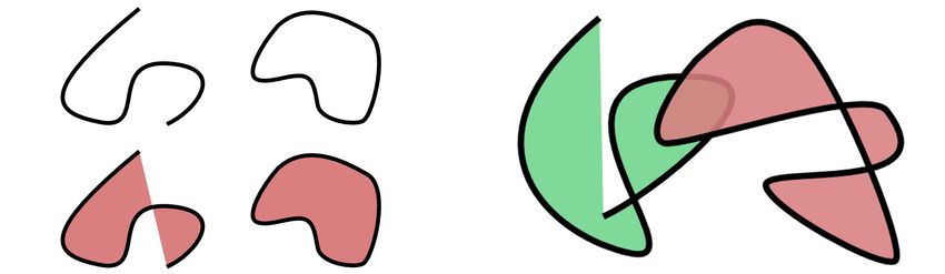
in their ability to model even basic topological constructs, such as Figure 2: The “SVG” representation, as used in Illustrator (except
joining an edge (or path) to the middle of another edge, or sharing for the LivePaint tool) and Inkscape. Left: Open and closed paths,
an edge between two faces. We further elaborate on such issues in filled or not. Right: Overlapping and self-overlapping paths.
the following section.
Planar maps [Baudelaire and Gangnet 1989] allow selected sets
of intersecting 2D paths to be used as the boundaries for defining
closed cells or faces, which can then be independently assigned at- ≡
tributes such as fill color. A difficulty of this approach is that the
planar map needs to be recomputed when the original 2D paths are
edited. By default, the need to compute a new planar map results (a) Shared edge in SVG (b) Shared edge + overlapping
in a loss of the attribute information stored with the original faces
of the planar map. In practice, it is in fact possible to devise heuris- Figure 3: The limitations of existing representations. SVG can-
tics for establishing correspondences between the new faces and the not represent two faces sharing a common edge as in (a), therefore
original faces, thereby allowing the attribute information to be car- must duplicate the shared edge. Planar maps can represent shared
ried over after edits [Asente et al. 2007]. Closely related to planar edges, but cannot represent overlapping faces, thus neither SVG
maps, [Takayama et al. 2013] proposes a curve network representa- nor planar maps can represent the illustration in (b).
tion well-suited for free-form sketching of patches decomposing a
3D mesh, useful for user-guided quad remeshing.
Stacking-based systems use a back-to-front rendering of layers to
3 Motivation and overview
designate the occlusion relationships among objects. However, il-
lustrations with cycles in the occlusion relations require developing In this section, we motivate the vector graphics complex (VGC)
work-arounds or alternate solutions. One approach is to develop and provide an intuition about its structure. This overview provides
local orderings [Wiley and Williams 2006; McCann and Pollard many of the insights needed to understand and implement the VGC.
2009] that allow for the layer orderings to be specific to a particular It also lays the foundation for understanding a formal description
area of the illustration. For cases where the illustration arises from rooted in graph theory and combinatorial topology that we provide
known 3D geometry, algorithms exist to identify the cycles and au- in the following section.
tomatically split a face so as to break the occlusion cycle [Eisemann Let us first recall the traditional vector graphics representation, that
et al. 2009]. Another solution that is particularly well suited to the we will refer to as “SVG” because of the XML Scalable Vector
depiction of knots and folds is to implement deformations to the 3D Graphics file specification of the same name. With SVG, a drawing
geometry so as to produce a desired local depth ordering as speci- is represented using building blocks called paths. A path is typi-
fied by a user [Igarashi and Mitani 2010]. Other work is aimed at cally a list of Bézier control points, that can be either closed or open.
the automatic extraction of 2D contiguous faces from underlying It has drawing attributes that indicate how it must be rendered, such
3D geometry [Karsch and Hart 2011]. as stroke width, stroke color, and fill color, as illustrated Figure 2.
Paths are defined independently of each other, which means that if
Our vector graphics complex can also be seen as an extension of
one path is dragged and dropped by the artist on top of another one,
stroke graphs [Whited et al. 2010; Noris et al. 2013], that repre-
they freely overlap and do not interact as shown in Figure 2.
sent the topology of a drawing by nodes (our vertices) and edges.
This topological information is used to establish automatic stroke This basic overlapping capability is a very desirable feature, since
correspondences between two keyframes of a traditional 2D ani- it allows the artist to freely edit the geometry of the paths and move
mation, and provide topology-aware interpolation of the strokes. the objects without any constraints. Nonetheless, there are cases
However, they never address the issue of the representation of faces, where it would be desirable to model interaction between paths.
and since their input is a scanned drawing, they never consider or A canonical example, also described in [Baudelaire and Gangnet
discuss overlapping edges (even though their data structure would 1989], occurs when the illustration represents two shapes that share
support it) or the usefulness of this structure as an interactive draw- a common partial contour or edge. In SVG, this must be represented
ing paradigm. as two independent closed paths, where the common section has
exactly the same geometry, as illustrated in Figure 3a.
A significant body of work on topological representations is
also relevant, including common choices such as, among others: While common tools such as Adobe Illustrator [Adobe Systems Inc.
winged-edge and half-edge structures; Nef polygons [Nef 1978]; 2013] or Inkscape [Inkscape 2013] provide convenient tools to
simplicial complexes, e.g., [De Floriani et al. 2003; De Floriani build such shapes (such as basic duplication or alignement features,
et al. 2010]; the selective geometric complex and structured topo- or the shape builder tool in Illustrator), the topological information
logical complex [Rossignac and O’Connor 1989; Rossignac 1997]; between the two shapes is still not explicitely encoded: the seman-
radial-edge structures [Weiler 1985]; and the adjacency and inci- tics of the intended illustration is not correctly represented. In prac-
dence framework [Silva and Gomes 2003]. Providing a meaningful tice, this means that the information about the common portion of
comparison with our proposed representation first requires defining the paths is duplicated, and editing its geometry is often tedious.
the VGC in detail and so comparisons of these representations with Typically, adding Bézier control points or editing tangents must be
the VGC are deferred until after we formally define the VGC, in performed twice (this limitation is demonstrated in the accompany-
section 4.4. ing video). Planar maps and their extension, dynamic planar mapse2 e3
v2 end
start
start e1
e1 end
v1 v3 e5 e2
f1 f2
e4
Figure 4: Two open edges e1 and e2 , and one closed edge e3 . e6
end e3
start
start end
start
v4
v1 Figure 6: Two faces f1 and f2 each defined by one cycle. The cycle
end e1 defining f1 is [(e1 , true); (e2 , false); (e3 , false); (e4 , true)], while
e5 end e2 the cycle defining f2 is [(e2 , true); (e6 , true)].
e4
v5
start start end e6
v3 e3
v2 that we call halfedges. Here, e represents an edge and β is a boolean
start indicating whether the edge should be considered with its intrinsinc
end orientation (from start to end, β = true), or with the opposite ori-
Figure 5: A VGC composed of vertices and edges only, similarly to entation (from end to start, β = false), as illustrated in Figure 6.
a stroke graph. v1 , v2 and v4 are each shared by three edges. Using several cycles for the same face makes possible to specify
holes in the face. Finally, we define the notion of Steiner cycle, that
is a cycle not defined by a list of halfedges, but defined by a single
vertex. A Steiner cycle makes possible to connect the end vertex of
(LivePaint in Illustrator), have been introduced as a solution to this an edge to the interior of a face.
problem. This, however, introduces other compromises, such as the
inability to have overlapping faces. While planar maps can faith- An artist creates edges and vertices by drawing strokes. He can
fully represent the semantics shown in Figure 3a, they cannot faith- choose whether intersections of strokes with existing edges must
fully represent the semantics of the illustration shown in Figure 3b. generate a new vertex and split the incident edges; or must simply
This second figure shares the same topology and can therefore be ignore the intersection and create overlapping edges, not topologi-
obtained from Figure 3a via simple editing of the geometry. This cally connected. Then, the artist can freely sculpt the geometry of
limitation seriously impairs artistic freedom and expressiveness. edges, or drag and drop cells. Also, he can use topological opera-
tors, for instance to glue two vertices or edges together, or cut a face
The vector graphics complex that we present is an alternative solu- into two faces by inserting a new edge. We refer the reader to the
tion, much closer to the spirit of SVG. Notably, it retains the ability accompanying video for a demonstration of this drawing paradigm.
to represent overlapping objects, and hence it is able to faithfully The cells are globally depth-ordered in a doubly-linked list, and we
capture the semantics of the illustration shown in Figure 3b without provide intuitive tools to alter this ordering, for instance to decide
duplicating any geometric information for the common section. which face is behind the other in Figure 3b.
Whereas in SVG the building block is the path, the VGC has build-
ing blocks called cells, of which there are three types: vertices, 4 Vector graphics complex
edges and faces. A vertex is simply a 2D point on the canvas, typ-
ically located where strokes meet or end. It can have drawing at- The vector graphics complex (VGC) is a non-manifold boundary
tributes such as a color and a radius size, but most often you would representation for 2D vector graphics, formally defined as a colored
prefer not to display it at all (just use it as a building block for incidence graph. In this section, we first describe the topology and
edges and faces). An edge is similar to an SVG path: it defines an geometry of this complex, and then propose an implementation.
oriented 2D curve on the canvas, for instance using Bézier control Finally, we assess its relevance by comparing it with existing non-
points. The significant difference with SVG paths is that edges do manifold representations.
not necessarily exist independently from other edges. For instance,
open edges must start at a start vertex, and end at an end vertex.
4.1 Topology
These vertices are stored as pointers in the edge implementation,
as illustrated in Figure 4. Therefore, as illustrated in Figure 5, two
or more open edges can be connected to each others by sharing a This section formally presents the theoretical foundations of the
common vertex, and manipulating this vertex would affect all inci- topology of a VGC. It does assume a background in graph theory,
dent edges. So far, this representation is identical to stroke graphs and a basic understanding of combinatorial topology. It is provided
[Whited et al. 2010], except that we do not order the incident edges for completeness, but the unfamiliar reader may safely skip it: the
counter-clockwise around a vertex. In addition, we define the no- actual implementation of a VGC and the remaining of the paper
tion of closed edge, which is an edge with no boundary vertex, as does not assume understanding of this section.
illustrated in Figure 4 (right). We note that it is allowed for an open
edge to have its start vertex be equal to its end vertex. At the con- Cell The topology of a VGC is composed of entities called cells.
trary to some existing representations, we only consider this to be a There exists three types of cells: vertices, edges, and faces, as illus-
special case of open edge and not a closed edge. trated in Figure 7.
Another difference with SVG paths is that VGC edges do not have
a color filling attribute: filling is done via the creation of faces, Incidence graph Each cell c is a colored node of a directed
an entity not supported by stroke graphs. A face is defined by its acyclic graph called the incidence graph, illustrated Figure 8. The
boundary via what we call cycles. A cycle is a a list of (e, β) pairs color indicates the type of the cell: vertex, edge, or face. To avoidv1 e1 v4 e7 v6 v2 f
e8
e4 e2 e3
e2 f1 f2 e6
f3
v1
v2 v3 v5 e1 e1 e2 e3
e3 e5
f =?
Figure 7: Two connected squares and an isolated disc represented
as a single VGC with 17 cells: six vertices v1 to v6 , eight edges (e1
to e7 are open, e8 is closed), and three faces f1 to f3 .
v1 v2
f1 f2 f3
Closed curve Filled Glued
e1 e2 e3 e4 e5 e6 e7 e8 Repeating e2 :
Repeating e3 :
v1 v2 v3 v4 v5 v6
Figure 9: Top: The incidence graph (without semantics) of a
Figure 8: The incidence graph (without semantics) corresponding Möbius strip. Bottom: To render it, one needs to decompose its
to the VGC illustrated in Figure 7. For clarity, we do not show here boundary into a closed curve. This requires to repeat (at least) one
the pointers from faces to vertices (can be deduced by transitivity). edge, and this choice is ambiguous: repeating e2 or repeating e3
give different rendering results when filling the face using the even-
odd winding rule.
confusion with the cell type “edge”, the oriented edges of the inci-
dence graph are called pointers. Thus, each cell c “points” to other
cells, and the set of these pointed cells is called the boundary of c,
denoted ∂c. The relation c ∈ ∂c0 is a strict partial order. We have:
• irreflexivity: c ∈
/ ∂c
• transitivity: if c ∈ ∂c0 and c0 ∈ ∂c00 then c ∈ ∂c00
• asymmetry (implied by first two): if c ∈ ∂c0 then c0 ∈
/ ∂c Figure 10: A VGC composed of three cells (two vertices and one
edge), and its incidence graph. The boundary of e is ∂e = {v1 , v2 }
Ambiguity of the incidence graph Unfortunately, this inci- ˆ = {(v1 , start), (v2 , end)}. This
while its semantic boundary is ∂e
dence graph does not encode enough information for our needs. additional semantics defines a topological orientation for the edge.
Indeed, rendering a 2D area of the plane defined by its possibly
self-intersecting boundary is traditionally done via the computation
of winding numbers, which requires as input one or several closed Hence, the topology of a VGC is formally defined as a colored di-
curves (“polygon contours” in OpenGL [Shreiner et al. 2004]). The rected multigraph G = (C, ∂), ˆ where C ⊂ N × N is a set of col-
incidence graph only gives a set of boundary edges, and converting
this set into closed curves is an ambiguous operation: it might in- ored cells (a cell has an id and a type), and ∂ˆ : C −→ P(N × N)
volve repeating edges, and the choice of the repeated edge affects is a map giving for each cell c the set of its colored pointers ∂cˆ (a
the rendering. This issue is illustrated in Figure 9 with the exam- pointer has a pointed id and a semantics). Obtaining ∂c from ∂c ˆ is
ple of a Möbius strip. To make the rendering of the VGC easier simply a projection onto the first component of the pair, an opera-
and consistent accross implementations, and to give the artist the tion that can be interpreted as “forgetting the semantics”. As usual
freedom to choose which closed curves must be used, we do not with projections, this is an irreversible operation: it is not possible
want this disambiguation to be automatically computed via geo- to resynthesize the semantics from ∂c, because it is an ambiguous
metric analysis of the edges. Rather, we directly encode this infor- operation, as illustrated in Figure 9.
mation in the incidence graph.
Helper Figure 11 (top) describes the semantics we would like to
Semantic boundary To do this formally, we add a color to each encode in the incidence graph of a Möbius strip. Obviously, this
pointer, that we call the semantics of the pointer. For instance, an is not practical, even more than formally, this semantics must be
open edge has exactly two pointers colored start and end (each encoded by a single integer per pointer. Instead, we introduce en-
pointing to a cell of type vertex) that defines a topological orien- tities that we call helpers, that are a higher level description of this
tation for the edge, as illustrated in Figure 10. Implementation- semantics, and can be seen as “meta-pointers”: in the same way
wise, we are just saying here that a pointer has a variable name. that a pointer points to a cell with semantics, a helper points to a
We define the semantic boundary of a cell c as the set of its col- set of cells with semantics. Figure 11 (bottom) illustrates this con-
ored pointers, denoted ∂c.ˆ For instance in Figure 10, we have cept. Appendix A proves that this description using helpers can be
ˆ = {(v1 , start), (v2 , end)}, while ∂e = {v1 , v2 }.
∂e converted into a proper colored incidence graph.e1 star
art to end t
e, from st
en
cycl
1st edge of v1
d
∅
t
3rd edge of cycle, from start to end star
f e2 end
2nd and 4t
h edge of cy ∅
cle, from en
v2
rt
d to start
sta
end
e3
e1 star
t
en
v1
d
Helper t
star
f e2 end
ˆ ≡ [[(e1 , T ); (e3 , F ); (e2 , T ); (e3 , F )]]
∂f
v2
rt
sta
end
e3
Figure 11: Top: The incidence graph (with semantics) of a Möbius
strip. The semantics disambiguates which edge must be repeated Figure 12: The complete description of the topology of a VGC rep-
twice, and specifies the traversal orientation of the cycle. Bottom: resenting a square with 4 vertices, 4 (open) edges, and 1 face.
The same semantics expressed with a helper. Here, T denotes the
boolean true, while F denotes false. By writing “∂f ˆ ≡”, we mean
that it is a convenient description of the semantic boundary of f : a
single cycle expressed by a sequence of edges with a specific orien-
tation.
Topological constraints In order to be valid, the semantic
boundary of the cells of a VGC must satisfy some constraints. We
decribe these constraints in the rest of this section, alongside a de-
scription of the semantics we attach to each type of cell.
Vertex ˆ = ∅.
A vertex v has a void boundary ∂v = ∂v
face f cycle 1 cycles 2 to 7 ∂f
Edge An edge is either open or closed. Figure 13: A valid face, with seven cycles. Cycle 1 represents its
external boundary (including a “crack”), and the six other cycles
• An open edge e has two pointers to vertices, one colored start represent holes (one of them being a single missing point in the
and the other colored end. We refer to them as vstart (e) and face, defined by the Steiner cycle).
vend (e), possibly equals.
ˆ = ∅.
• A closed edge e has a void boundary ∂e = ∂e
and called a non-simple cycle otherwise (i.e., when defined as a se-
Halfedge A halfedge h = (e, β) is a pair composed of an edge quence of open halfedges).
e and a boolean β representing a chosen orientation of the edge. If
e is a closed edge, then h is said to be a closed halfedge. If e is an Face The semantic boundary of a face f is defined by a sequence
open edge, then h is said to be an open halfedge, and we define: (γi )i∈{1,..,m} of m ≥ 0 cycles. There are no other restrictions. For
if β = true if β = false instance, even though a face without cycle is rather useless for vec-
tor graphics, it is valid and theoretically justified in [Dalstein et al.
vstart (h) = vstart (e) vstart (h) = vend (e) 2014]. Most other oddities, such as repeating an edge three times
vend (h) = vend (e) vend (h) = vstart (e) or more are not only valid and theoretically justified, but actually
useful (cf. Figure 19, middle and right). The cycles must not nec-
Cycle A cycle γ is either: essarily be disjoint: they can share common vertices or edges (cf.
Figure 13). The boundary ∂f of a face is the set of all the edges
• A single vertex v, or and vertices involved in the cycles. Intuitively, if only one cycle
• A sequence (hi )i∈{1,..,n} of n > 0 halfedges satisfying: is given, then it defines the contour of the face. If more than one
is given, then it defines holes inside this face. Figure 12 illustrates
– h1 is a closed halfedge and ∀i ∈ {1, .., n}, hi = h1 , or the topology of a face with a single cycle. A face can represent a
non-orientable surface, like the Möbius strip in Figure 11.
all halfedges are open, and
– vstart (h1 ) = vend (hn ), and
∀i ∈ {1, .., n − 1}, vend (hi ) = vstart (hi+1 ) 4.2 Geometry
There are no other restrictions. For instance, a cycle may repeat any The previous section defined the topology of a VGC, a combinato-
number of vertices or edges with arbitrary orientation. A cycle is rial structure representing the neigbourhood relationships between
called a Steiner cycle when it is defined as a vertex, called a sim- abstract cells. This section defines the geometry of a VGC, i.e., how
ple cycle when it is defined as (possibly repeated) closed halfedge, each cell c is realized as a pointset |c| ⊆ R2 .Vertex The geometry of a vertex v is a point pv ∈ R2 , and we We do not described the Curve class since it is up to each applica-
define |v| = {pv }. tion to decide on a curve representation adapted to its specific con-
text. For instance, an existing vector graphics system with extensive
support of Bézier curves may use Bézier curves. For our prototype,
Open edge The geometry of an open edge e is a continuous curve
we opted for a simpler dense polyline representation. On top of this
Γe : [0, 1] → R2 , satisfying Γ[0] = vstart (e) and Γ[1] = vend (e).
core structure, more drawing attributes can be added for fine control
We define |e| = Γe ((0, 1)).
on rendering. For instance, we added vertex radius, variable edge
width, cell color (possibly transparent), and edge junctions style
Closed edge The geometry of a closed edge e is a continuous (mitre join or bevel join).
closed curve Γe : S 1 → R2 , where S 1 is the unit circle. We define
|e| = Γe (S 1 ). 4.4 Comparison with other representations
Face The geometry of a face f is defined by a winding rule We have already discussed (cf. Section 2) the limitations of the
R ⊆ N, from which can be defined a pointset |f | ⊆ R2 that SVG representation [SVG Working Group 2011], the limitations
we detail in the remainder of this paragraph. For each simple of planar maps [Baudelaire and Gangnet 1989; Asente et al. 2007]
or non-simple cycle γ of a face f , we define the closed curve (also shared by Nef polygons [Nef 1978]), and the connection be-
Γγ : S 1 → R2 by concatenating the functions Γe of all edges tween the VGC and stroke graphs. In this section, we compare the
e involved in the cycle. We denote by |γ| = Γγ (S 1 ) the set of VGC to representations that belong to the the realm of topologi-
points p ∈ R2 belonging to the cycle. If γ is a Steiner cycle
S defined cal modeling. We took inspiration from these existing topological
by v, we simply define |γ| = |v|. We define |∂f | = γ∈∂f ˆ |γ|, structures, and adapted them to the problem at hand, resulting in a
and we note that it is equal to c∈∂f |c|. For each p ∈ R2 \|γ|,
S pictorial space that combines the genericity of non-manifold non-
orientable 3D topology with the flexibility of 2D geometry. A gen-
Γγ defines a winding number Nγ (p) ∈ N (cf. [Edelsbrunner and
eral observation is that in 2D, there is no need to explicitly describe
Harer 2010, p12]). If γ is a Steiner cycle, we define Nγ (p) = 0.
the geometry of surfaces, since it is completely described by the
We define,Pfor each p ∈ R2 \|∂f |, the total winding number
geometry of its boundary and a winding rule. We take advantage of
Nf (p) = γ∈∂f ˆ Nγ (p) obtained by summing the winding num-
this in order to propose a simpler ad-hoc data structure.
bers for each cycle of f . Finally, |f | is defined as the pointset
{p ∈ R2 \|∂f | s.t. Nf (p) ∈ R}. Our implementation uses the Well-known topological representations include the winged-edge,
OpenGL GLU polygon tesselator [Shreiner et al. 2004] with the half-edge and quad-edge data structures, combinatorial maps, and
even-odd winding rule, but other rules could be considered as well. cell-tuples. These are not suitable, since they cannot represent
non-orientable surfaces. The necessity to represent such topologies
4.3 Implementation comes from our requirement to have a data structure closed under
the glue operation (more detail in Section 5). However, we note that
Despite the possibly discouraging formalism, the implementation Guibas and Stolfi [1985] define an edge algebra similar to ours.
is surprisingly easy and we present here our C++ class structure. The selective geometric complex and the structured topological
c l a s s C e l l { s e t < C e l l ∗> s t a r ; } ; complex [Rossignac and O’Connor 1989; Rossignac 1997] are both
c l a s s Vertex : public Cell { Point p ; }; a source of inspiration for the VGC and hence have a lot in common
c l a s s Edge : public Cell { Vertex ∗ s t a r t ; with it. However, even though the STC cyclically orders the faces
V e r t e x ∗ end ; around an edge, neither the SGC nor the STC cyclically orders the
Curve c u r v e ; }; edges bounding a face. Such cycles are required for the unambigu-
s t r u c t H a l f e d g e { Edge ∗ e d g e ; b o o l b ; } ; ous computation of winding numbers, thus the SGC and STC as
s t r u c t Cycle { Vertex ∗ s t e i n e r ; currently defined are not directly suitable for our purpose.
vector h a l f e d g e s ; } ; Suitable representations would include the radial-edge structure
c l a s s F a c e : p u b l i c C e l l { v e c t o r < Cycle > c y c l e s ; } ; [Weiler 1985], extensions and/or specialization [Gursoz et al. 1990;
Lee and Lee 2001; Marcheix and Gueorguieva 1995], as well as
As detailed in Section 4.1 and 4.2, a vertex is simply a 2D position, Nef polyhedra [Granados et al. 2003; Nef 1978], generalized maps
an edge is a 2D curve pointing to its ordered end vertices (if any), [Lienhardt 1994], and the handle-cell data structure [Pesco et al.
and a face is a list of cycles, where a cycle is either a list of halfedges 2004]. However, these representations are more complex to under-
or a single vertex. Checking if an edge e is open is simply done stand and implement than the VGC, mainly because they target 3D
via if(e->start) (e->start and e->end are both NULL CAD applications and hence have a richer structure to support 3D
for closed edges). Similarly, checking if a cycle g is a Steiner cycle geometric queries and boolean operations that are less a concern
is simply done via if(g->steiner), in which case the vector for us. [Gursoz et al. 1991] describes a representation very similar
of halfedges is empty. to the VGC, but the authors do not provide any details on an actual
data structure, and only consider planar surfaces, and as such do not
The star of a cell c is defined by the set of cells whose boundary consider edges shared more than two times by the same face.
contains c, i.e. star(c) = { c0 | c ∈ ∂c0 }. While not stricly
required (redundant information), finding the star of a cell is a very Simplicial complexes [De Floriani et al. 2010] are limited to faces
frequent query, and storing it in the datastructure makes this query bounded by exactly three edges, which is not expressive enough
constant time instead of linear in the number of cells (the same way for vector graphics. They can be decomposed into nearly manifold
as implementations of directed graphs often contains back-pointers parts equivalent to our cells [De Floriani et al. 2003], but this still
to parent nodes). However, we do not store any semantics in the requires the underlying triangulation, unlike our approach. The ad-
star and store them indistinctivily in a set. If semantics is needed, jacency and incidence framework described in [Silva and Gomes
then the semantic boundary of the star cells of can be inspected 2003] is a pure incidence graph, and then as we discussed ear-
to retrieve it. We tried to encode semantics for the star, but found lier does not contain enough information to disambiguate winding
that it makes maintaining the consistency of the data structure much numbers, as required for the 2D rendering of our faces. The VGC
harder, and that it was not worth the marginal efficiency gain. extends it with semantics to solve this issue.5 Topological operators Glue UnGlue
Since topology lies at the heart of the vector graphics complex, and
that we aim at porting topological modeling into the the realm of Glue UnGlue
2D vector graphics, it is highly desirable to be able to manipulate in
an intuitive fashion this topology, using topological operators. Tra-
ditionally, such operators are described as Euler operators, since as
a safety check one ensures that they are compatible with an Euler Glue
formula, linking the number of cells of each type, and topologi- UnGlue
cal quantities such as the number of connected components and the
number of holes. Designing an Euler formula in the case of our Glue
non-manifold, non-orientable, mixed-dimensional objects is likely
possible and definitely interesting, but it is far from trivial and rather UnGlue
irrelevant as a safety check. Instead, one just has to ensure that the
topological constraints, or invariants using a programming termi-
algorithm UnGlue
nology, are preserved. These invariants for our implementation are:
• Vertex: no topological invariants.
Glue
• Edge: the start and end vertices are either both non-NULL
valid pointers (open edge), or both NULL (closed edge). algorithm
• Halfedge: edge is a non-NULL valid pointer.
Figure 14: Examples of glue and unglue operations on vertices,
• Cycle: one of the following is true: edges, and a set of cells (bottom-right).
– steiner is a valid non-NULL pointer and
halfedges is empty.
5.1 Creation and deletion operators
– steiner is NULL, halfedges has a size n > 0, and
one of the following is true: Creating a vertex or a closed edge does not requires special care.
Creating an open edge requires refering to existing start and end
∗ halfedges[0] is a valid closed halfedge, and vertices. These topological operators are automatically invoked
for all i ∈ {1, . . . , n − 1}, when the user draws a stroke, as detailed in Section 7. Creating
halfedges[i] == halfedges[0] a face requires as input its list of valid cycles, and obtaining these
valid cycles from intuitive user input is still an open problem. Cur-
∗ halfedges only contains valid open halfedges, rently, we ask the user to select a set of edges, which is automat-
and for all i ∈ {0, . . . , n − 1}, ically converted to cycles. This is not only tedious for the user,
but more importantly we recall that this conversion is ambiguous.
halfedges[i].end() == When ambiguity is detected, we abort the operation. To achieve
halfedges[(i+1) % n].start() faces such as the Möbius strip in Figure 9, one option for the user is
to explicitly draw the repeated edge twice (left), fill this face (mid-
• Face: Every cycle in cycles is valid.
dle), then glue together the two repeated edges (right). We leave as
In addition, since our implementation includes the backpointers future work the automatic detection of potential faces, which would
star, every cell c must satisfy: enable “click to fill” tools that are common for faces in planar maps.
To delete a cell, we first recursively delete its star, otherwise the
• ∀c0 ∈ ∂c, c ∈ c0 .star VGC would become invalid. We refer to this topological operation
• ∀c0 ∈ c.star, c ∈ ∂c0 as a “hard delete”. However, by default our delete command enacts
a “smart delete”, whose semantics are designed to better reflect a
A key feature of these invariants is that they can be verified effi- user’s intentions. If we consider the case of a vertex, v, with two
ciently and robustly without geometric computations. In this sec- incident edges, e1 and e2 , and a user that chooses to “delete” v, the
tion, we informally present the reversible operators create/delete, intended outcome is more likely to be a single longer edge e3 that
glue/unglue and cut/uncut. They provably maintain all topological is the geometric union of v, e1 and e2 , as opposed to an alternative
invariants and are detailed in [Dalstein et al. 2014]. They can be scenario that deletes each of v, e1 , and e2 . The intended outcome is
intuitively combined together by the artist to achieve the intended given by the topological operation “uncut at v”, as will be detailed
topology. In fact, gluing and cutting are not only useful operations, later. However, it may not always be possible to uncut at a given
but have theoretical roots in algebraic topology. For instance, the vertex v, such as is the case when there are three or more incident
proof of the classification of closed two-manifolds involves “cut- edges. The semantics of our “smart delete” are thus defined by
ting” the given manifold until the manifold is represented as a fun- “uncut if possible; otherwise, hard delete”.
damental polygon. By gluing together the edges of this polygon,
we re-obtain the original manifold. The VGC is a superset of fun- 5.2 Glue and unglue operators
damental polygons and is furthermore closed under gluing, which
proves that the VGC can represent any closed two-manifold, includ- The glue operator on vertices and edges, as well as the unglue op-
ing non-orientable surfaces such as the Klein bottle in Figure 1. erator on vertex, edge, or set of vertices and edges are illustrated
More theoretical considerations show that the VGC can represent in Figure 14. Gluing two vertices is the equivalent of the opera-
any regular non-manifold two-dimensional topological space [Dal- tion join in existing vector graphics software, where two paths are
stein et al. 2014]. appended by gluing together two selected path end-nodes. How-Cut UnCut
Cut UnCut
Cut UnCut
(Steiner)
Cut UnCut Figure 16: The effect of a global “uncut”. Left: Original VGC.
Right: VGC resulting from applying “select all” and then “uncut”.
Cut UnCut
(failure) holes, then one may decide to transfer these holes either to f1 or
f2 , which requires geometric heuristics. Designing a set of infal-
lible heuristics is unfortunately not possible because the boundary
of a hole is allowed to overlap the boundary of f , or can even be
Cut
UnCut completely outside f .
Uncutting is the reverse operation: the user chooses a cell c (a ver-
tex or an edge) where to uncut, and the operator merges this cell
Figure 15: Examples of cut and uncut operations on vertices and with its star to obtain a larger cell. Therefore, it can be seen as a
edges. The third operation on the right column illustrates uncutting “smart delete” or a “local simplification” operation. This operation
a Steiner vertex from a face. It is topology equivalent to the fifth has a significant theoretical relevance and we refer to this as atomic
operation on the same column. The fifth example on left column is simplification [Dalstein et al. 2014]. While it is always possible to
a failure case, when the cut algorithm transfers the “hole cycle” to cut any given cell, i.e., a face or an edge, it is not always possible to
the wrong face (shown in red). This happens because the cut oper- uncut at a given cell c. Specifically, this is only possible if c “could
ator is actually ambiguous and disambiguation require geometric have been obtained via a cut”. Equivalently, it is only possible if
heuristics to capture the user’s intent. the union of c with its direct star is a manifold space [Dalstein et al.
2014]. For instance, if a vertex v has three incident edges, then
the union of v with its direct star (in this case the incident edges)
is non-manifold, and hence uncutting at v is not possible. Surpris-
ever, with such a classical join operation, the selected end-nodes ingly, uncutting is “conceptually simpler” than cutting: it is never
are transformed into a middle Bézier control point that cannot be ambiguous and does not rely on any geometric computation.
joined again to create three-way junctions. In contrast, the VGC
is closed under the glue operation: any two vertices, or two open Once the uncut operator is implemented both for a single vertex
edges, or two closed edges can always be glued. In fact, gluing two and a single edge, it can be trivially extended to a set of cells: sim-
edges is ambiguous and is only a convenient operation provided for ply uncut all selected edges, then uncut all selected vertices. This
the user. Our implementation uses a simple heuristic to predict the is a powerful topological simplification operator, as illustrated in
most relevant orientation for the selected edges and then calls the Figure 16: performing this operation on the whole VGC is equiv-
unambiguous glue halfedges topological operation. This first glues alent to the simplification operation described in [Rossignac and
their respective start and end vertices together, and only then glues O’Connor 1989]. We conjecture that it results in a unique minimal
the edges together. The unglue operation is the reverse operation, decomposition [Dalstein et al. 2014].
where a vertex or an edge is duplicated as many times as necessary.
Ungluing a vertex involves first ungluing its incident edges. 6 Depth ordering
5.3 Cut and uncut operators An important consideration in vector graphics is the ability to or-
der cells from back to front and paint them appropriately. In this
section, we describe how this operation is supported with the VGC.
The results of the cut and uncut operators are illustrated in Fig- Each cell in a VGC (e.g., vertices, edges, and faces) is assigned a
ure 15. Cutting an edge e is the equivalent of inserting a new con- unique depth order. The order is maintained via a doubly-linked list
trol point in a SVG path: given a 2D position p on the geometry containing all the cells, where the ‘top’ cell of the list will be drawn
of an edge e, it creates a new vertex v at position p, and cuts e last and will therefore occlude other parts of the drawing. When a
into two edges e1 and e2 separated by v. If e was a closed edge, new cell c is created, it is by default inserted just below the lowest
then it becomes an open edge with its start and end vertices equal cell in its boundary ∂c.
to v. Cutting a face f is similar: given a curve Γ starting and end-
ing on ∂f , it cuts the face into two faces f1 and f2 , separated by Further alterations of the depth ordering are supported by allow-
a new edge e whose geometry is Γ. This may involve cutting first ing the user to raise a selected cell, c. A trivial implementation
∂f to create the end vertices of e if they do not already exist. Al- of raise would be to simply swap the depth order of c and the cell
ternatively, if Γ starts and ends at two different cycles of f (cf. immediately above it in the depth order, cnext , as depicted in Fig-
Figure 15, bottom-left), then instead of cutting f into f1 and f2 , it ure 17. However, this typically fails to capture the user’s intention:
simply merges the two cycles into one by concatenating them with there may be no visible change as a results of the raise, and, if a
the halfedges (e, true) and (e, false). Finally, a face can also be face or edge is selected, the commonly-desired semantics is to have
cut by a closed curve contained in its interior, or by a point p (via a vertices remain on top of the edges and faces that they help de-
Steiner cycle). In the general case, cutting a face is ambiguous and fine, and edges to remain on top of the faces that they help define.
is therefore less trivial than one might think [Dalstein et al. 2014]. These semantics are implemented by Algorithm 6.1 and illustrated
A simple example is given in Figure 15 (failure case): if f contains in Figure 17. The lower operation is the counterpart to raise and is∂c ∂c0
bottom top
c cnext c0
C+
Figure 17: Raising a cell.
Figure 19: Examples of non-manifold topologies where an edge
has three “face uses”. These uses may be by the same face (middle
and right), and part of a hole (right)
Figure 18: An example of the flexible occlusion interactions en-
abled by the VGC.
implemented in a largely symmetric fashion, where the directions
are reversed and ∂c is replaced by star(c).
Algorithm 6.1: R AISE(selected cell c)
search from bottom to find c
compute C + = subset of (c ∪ ∂c) that is above c
search up from c for the first cell c0 satisfying: Figure 20: A user experimenting with the possibilities offered by
c0 6∈ ∂c AND geometry of c0 intersects with c invisibe cuts and depth ordering.
move C + above the highest element of (c0 ∪ ∂c0 )
The ability to manipulate depth orderings for components within
objects and between objects allows for partial orderings such as Creating faces and holes: Faces and holes can be created in multi-
that shown in Figure 18. One arm of the glasses is stacked so as to ple ways, as demonstrated in the videos associated with this paper.
be behind the face while the other remains in front, along with the Faces are created by selecting the edges that will serve as a bound-
rest of the frame. More examples involving depth manipulations ary. For faces where this does not yield a unique cycle, we require
are shown in Figure 1 and in the accompanying video. that the face be constructed through intermediate steps. Multiple
holes can be added to a face, with the resulting fill determined by
7 User interface their winding number, as shown in Figure 19.
Steiner cycles: Steiner cycles are created by selecting the face and
Many aspects of the user interface can be readily understood from the vertex to add as Steiner cycle. Its primary use is to connect
the videos associated with this paper. In what follows we provide a the end vertex of an edge to the interior of a face. Dragging the
summary of the fundamental concepts and operations. face would also drag this end vertex, since it translates the whole
Edge design: Hand-drawn strokes are the primary method for cre- face boundary. If desired, Steiner cycles can also be used to topo-
ating edges. An open stroke drawn on the canvas creates an edge logically connect two faces that do not share a common edge. By
with start and end vertices. Edges can be drawn in a standard fixed- sharing a common Steiner cycle, they can still be dragged indepen-
width mode, or their width can vary as a function of stylus pressure. dently, but form a single connected component.
Edges are represented as a densely sampled polyline and can be Performance: The performance of our implementation is cur-
reshaped using a sculpting tool, either by locally dragging points, rently limited by the naive dynamic tesselation that we perform for
smoothing, or editing the width of the curve. If new intersections each render. Edges are rendered according to their width attribute
occur when sculpting an edge, they are ignored and never lead to through generation of quadrilaterals that are centered around the
the creation of a new vertex. The user can always manually insert a polyline that represents the edge path, and these are not cached be-
vertex at any given intersection. tween renders. Similarly, all faces are retesselated for each render.
Intersections and snapping behavior: If desired, edges can be
drawn in a mode analogous to working with planar maps. This 8 User feedback
automatically cuts intersected edges and faces, and cuts the drawn
edge at self-intersections. This mode can be enabled or disabled in Our prototype has been informally tested by five users ranging from
the GUI by toggling an always-visible icon. A snapping behavior novice to professional artists. Using this feedback, we provide
can also be toggled: if enabled, end points of strokes snap to exist- an initial assessment of the usability of the SVG by non-technical
ing vertices if within a distance . Self-intersection junctions can users.
also snap to each other, thereby allowing multiple approximately
colocated self-intersections to automatically coalesce into a single Users consistently report that using the VGC is significantly differ-
junction. ent from current SVG tools, and that it opens exciting new creativeFigure 22: Three more vector illustrations designed using the
VGC. The ellipse surrounding the top illustration is a single edge
Figure 21: The VGC can be used for abstract art or stylized figu- whose width was sculpted. Examples drawn by Estelle Charleroy.
rative art. Examples drawn by Etienne Colas.
supported, the VGC offers little support for geometric operations
workflows. Due to this novelty, the first impressions are generally such as boolean operations. The parameterization of VGC faces
quite enthusiastic. The topological operations such as glue, unglue, is left as a separate problem; our current system does not support
uncut (directly via a tool “simplify”, or indirectly when “deleting” texture-mapped faces. While a parameterization could be estab-
a cell) are appreciated and readily adopted. Interestingly, one of lished via triangulation based on a particular geometric configura-
the most appreciated features is the ability to sculpt the interior of tion, future geometric edits may then become problematic.
edges via local dragging or smoothing. Our free-form width editing
It would be useful to extend or augment the VGC to support vector
is reported to be especially useful (see Figure 22).
graphics animation, where time is the additional dimension. In the
Concerns have also been raised. Not surprisingly, one of the most accompanying video, we in fact demonstrate that VGCs can triv-
disliked aspects of the prototype is the necessity to select all the ially be animated by deforming their geometry in a consistent fash-
boundary edges to create a face. Sometimes, due to an unclean ion as long as their topology does not change. However, topology
topology and tiny edges, this is hard to achieve. Also, rendering changes in the time dimension are left for future work.
artefacts at junctions (see Section 9) and the difficulty to sculpt in-
Another concern is that even though using VGCs appears reason-
cident edges across a vertex, specifically to get a smooth transition,
ably intuitive, they are still a more complex structure than SVG,
have been mentioned. Finally, users currently tend to stay in the
which may cause confusion and frustration for artists used to the
(default) “planar map” mode, and hence fail to see the advantage
classical representation. For example, a user cannot “uncut” a ver-
that overlapping faces offer. One user experimented with invisible
tex shared by more than three edges or an edge shared by three or
cuts and depth ordering (Figure 20), but reported difficulties to mas-
more faces. A vertex that is a Steiner cycle of a face can be moved
ter the feature. However, we believe that further interface revisions
outside of the face, which can be unintuitive. Constraints could be
and video tutorials would ease the learning experience.
added to resolve this, but this then removes the independence of the
topology and the geometry. Representing an opaque disc involves
9 Limitations and future work only one path with SVG (a path with a fill color), while it involves
two cells with the VGC (a closed edge and a face whose boundary
The decorrelation of geometry and topology is a powerful means is this edge). However, the application could easily be adapted to
of representing the topology of visual objects as they appear in the provide further abstractions and tools making the VGC more artist-
mind’s eye. As a result, it is left to the user to maintain any desired friendly. For instance, the fill-color property can be simulated by
consistency between geometry and topology of VGCs. This can be automatically creating a face (and a closing edge for open edges)
a limitation in some cases. While the input we provide to the tesse- for every edge in the complex. We believe that the benefits of the
lator is the same as used for SVG and is therefore known to be well VGC largely outweight the added complexity.can be drawn with vector graphics, including 2D projections of 3D
? UnGlue objects with imprecise or incomplete geometry, non-manifold sur-
faces of arbitrary genus, non-orientable surfaces, and overlapping
faces. VGC neatly separates the geometry of vector graphics ob-
jects from their topology, making it easy to deform objects geomet-
rically in interesting and intuitive ways; and to edit their topology
UnGlue UnGlue with reversible and provably-correct operators. Components of ob-
jects can exist on different layers, which allows for occlusion be-
haviors to be defined for individual object components rather than
objects as a whole. Finally, the explicit representation of multiway
Figure 23: A user cannot achieve the “partial unglue” operation joins can be leveraged to improve rendering.
(shown in the top left) in one step. It can be accomplished indirectly
via a sequence of unglues and reglues. 11 Acknowledgements
We thank Estelle Charleroy, Etienne Colas, and other anonymous
artists for their invaluable user feedback. We also thank all the re-
viewers for their precious comments that have helped improving
the article in many ways. Part of this work was supported by ERC
No join Bevel join Bevel join Miter join Miter join Advanced Grant "Expressive", by GRAND, and by NSERC.
(Illustrator) (VGC) (Illustrator) (VGC)
Figure 24: Illustrator (except when using LivePaint) cannot rep- References
resent multiway joins, thus fails to render them correctly: incident
faces are rendered independently. With the VGC, we are aware of A DOBE S YSTEMS I NC ., 2013. Adobe Illustrator: Help and tutori-
multiway joins and hence can improve the rendering, as illustrated als.
here with the two common styles “bevel” and “miter”.
A SENTE , P., S CHUSTER , M., AND P ETTIT, T. 2007. Dynamic
planar map illustration. ACM Trans. Graph. 26, 3 (July), 30:1–
30:10.
Some desired topological operations must currently be performed
using multiple steps, such as the “partial unglue” shown in Fig- BAUDELAIRE , P., AND G ANGNET, M. 1989. Planar maps: An
ure 23. We expect that it is possible to create macros for many such interaction paradigm for graphic design. In Proceedings of the
operations. SIGCHI Conference on Human Factors in Computing Systems,
ACM, New York, NY, USA, CHI ’89, 313–318.
One advantage of the VGC over traditional vector graphics is that,
as with planar maps, it enables the representation of multiway joins DALSTEIN , B., RONFARD , R., AND VAN DE PANNE , M. 2014.
(three or more edges sharing a common vertex). As shown in Fig- Point-curve-surface complex: A cell decomposition for non-
ure 24, being aware of multiway joins (as opposed to emulating manifold two-dimensional topological spaces. Tech. rep., Uni-
them via duplicated edges) makes it possible to inform the render- versity of British Columbia.
ing for better results. However, we note that this is a double-edged D E F LORIANI , L., M ORANDO , F., AND P UPPO , E. 2003. Rep-
sword: in the most general case, the correct rendering of multi- resentation of non-manifold objects through decomposition into
way joins is a rather difficult and open problem, especially when nearly manifold parts. In Proceedings of the Eighth ACM Sym-
the incident edges have different and possibly non-uniform widths posium on Solid Modeling and Applications, ACM, New York,
and colors. This leads to various visible artefacts in our prototype. NY, USA, SMA ’03, 304–309.
In Figure 25, we illustrate a typical artefact that occurs due to the
overlapping ability of VGC cells and the presence of zero-width or D E F LORIANI , L., H UI , A., PANOZZO , D., AND C ANINO , D.
transparent edges. 2010. A dimension-independent data structure for simplicial
complexes. In Proceedings of the 19th International Meshing
Roundtable, Springer Berlin Heidelberg, 403–420.
10 Conclusion
D URAND , F. 2002. An invitation to discuss computer depiction.
We have introduced the Vector Graphics Complex, a novel and pow- In Proceedings of the 2nd International Symposium on Non-
erful data structure for topology-aware design of 2D illustrations. photorealistic Animation and Rendering, ACM, New York, NY,
VGC is a superset of multi-layer vector graphics, planar maps and USA, NPAR ’02, 111–124.
stroke graphs, which significantly extends the range of objects that
E DELSBRUNNER , H., AND H ARER , J. 2010. Computational
Topology: An Introduction. Applied mathematics. American
Mathematical Society.
E ISEMANN , E., PARIS , S., AND D URAND , F. 2009. A visibil-
ity algorithm for converting 3D meshes into editable 2D vector
graphics. ACM Trans. Graph. 28, 3 (July), 83:1–83:8.
G RANADOS , M., H ACHENBERGER , P., H ERT, S., K ETTNER , L.,
Figure 25: Left: To obtain a self-overlapping object, one “invisible M EHLHORN , K., AND S EEL , M. 2003. Boolean operations
edge” is necessary, to define two faces with different depth orders. on 3D selective Nef complexes: Data structure, algorithms, and
Right: This ordering implies that the red edge is below the yellow implementation. In Algorithms - ESA 2003, vol. 2832 of Lecture
face. Depending on the geometry of the invisible edge, this situation Notes in Computer Science. Springer Berlin Heidelberg, 654–
often leads to artefacts in our implementation. 666.You can also read