Why Noether's Theorem applies to Statistical Mechanics
←
→
Page content transcription
If your browser does not render page correctly, please read the page content below
Why Noether’s Theorem applies to Statistical Mechanics

                                                                                              Sophie Hermann∗ and Matthias Schmidt†
                                                                                             Theoretische Physik II, Physikalisches Institut,
                                                                                            Universität Bayreuth, D-95447 Bayreuth, Germany
                                                                                                      www.mschmidt.uni-bayreuth.de
                                                                                                        (Dated: 7 November 2021)
                                                                       Noether’s Theorem is familiar to most physicists due its fundamental role in linking the existence
                                                                    of conservation laws to the underlying symmetries of a physical system. Typically the systems are
                                                                    described in the particle-based context of classical mechanics or on the basis of field theory. We
arXiv:2109.10283v3 [cond-mat.stat-mech] 8 Nov 2021

                                                                    have recently shown [Commun. Phys. 4, 176 (2021)] that Noether’s reasoning also applies to thermal
                                                                    systems, where fluctuations are paramount and one aims for a statistical mechanical description.
                                                                    Here we give a pedagogical introduction based on the canonical ensemble and apply it explicitly
                                                                    to ideal sedimentation. The relevant mathematical objects, such as the free energy, are viewed
                                                                    as functionals. This vantage point allows for systematic functional differentiation and the resulting
                                                                    identities express properties of both macroscopic average forces and molecularly resolved correlations
                                                                    in many-body systems, both in and out-of-equilibrium, and for active Brownian particles. To provide
                                                                    further background, we briefly describe the variational principles of classical density functional
                                                                    theory and of power functional theory.

                                                                        I.   INTRODUCTION                                   In practice the theorems are usually applied to the ac-
                                                                                                                         tion functional in a Lagrangian or Hamiltonian theory.
                                                        Symmetries and their breaking in often stunningly                This strategy is not of mere historic interest, as much
                                                     beautiful ways are at the core of a broad range of phenom-          active current research is being carried out, see e.g. re-
                                                     ena in physics, from phase transitions in condensed mat-            cent developments that addressed the action functional
                                                     ter to mass generation via the Higgs mechanism. Most                for systems that include random forces [4–6] and work
                                                     readers will be very familiar with the importance of sym-           that shows, starting from the symmetry of an action func-
                                                     metry operations, including complex operations such as              tional, that the thermodynamic entropy can be viewed as
                                                     CPT-invariance in high energy physics as well as the sim-           a Noether invariant [7–9]. However, from a mathematical
                                                     ple challenge of centering the webcam while having mir-             point of view, Noether’s theorem is actually not restricted
                                                     roring switched off in a video call.                                to the specific case of the action integral. The theorem
                                                        The exploitation of the underlying symmetries of a               rather applies to a much more general class of function-
                                                     physical system is an important and central concept that            als, where it specifies general consequences of invariance
                                                     allows to simplify the mathematical description and ar-             under continuous symmetry transformations.
                                                     guably more importantly to gain physical insights and                  We recall some basics of functional calculus. A func-
                                                     achieve an understanding of the true mechanisms at play.            tional is a mathematical object that maps an entire func-
                                                     This is what the mathematician Emmy Noether did in                  tion, i.e. the function values together with the corre-
                                                     her groundbreaking work in functional analysis early in             sponding values of the argument, to a single number. A
                                                     the twentieth century [1].                                          popular introductory example of a functional is the defi-
                                                        Noether analyzed carefully the changes that occur                nite integral, say over the unit interval from 0 to 1. When
                                                     upon performing a symmetry operation on a system. Her               viewed as a functional, the definite integral accepts the
                                                     work solved the then open deep problems of energy con-              integrand (a function) and it returns a number (the area
                                                     servation in general relativity, as the new theory of grav-         under the curve that the function represents). Although
                                                     ity that Einstein had just formed. Noether considered the           the functional point of view might appear slightly uncom-
                                                     formulation of general relativity via Hilbert’s action inte-        mon (or even trivial in this case), the inherent abstract
                                                     gral, which is a formal object –a functional– that gener-           concept allows to formulate very significant insights and
                                                     ates Einstein’s field equations. Nowadays Noether’s the-            use powerful mathematical techniques of variational cal-
                                                     orems [1–3] are widely known and used to connect each               culus which can be straightforwardly and widely applied.
                                                     continuous symmetry of a system with a corresponding                   The occurrence of functionals in physics is not re-
                                                     conservation law. Noether’s work therefore forms a staple           stricted to the study of behaviour at very large length
                                                     of physics, relevant from introductory classical mechan-            scales, such as that of the cosmos in the case of general
                                                     ics to advanced theories such as the standard model of              relativity, or to very high energies, as is the case for fun-
                                                     high energy particle physics.                                       damental theories of elementary particles. In fact the
                                                                                                                         mathematical concept of a functional dependence is very
                                                                                                                         general. Hence there is an according wide variety of ob-
                                                                                                                         jects in physics, such as e.g. the partition sum and the
                                                     ∗   Sophie.Hermann@uni-bayreuth.de                                  free energy in Statistical Mechanics that can be viewed as
                                                     †   Matthias.Schmidt@uni-bayreuth.de                                being a functional [10–13]; we give an introduction below.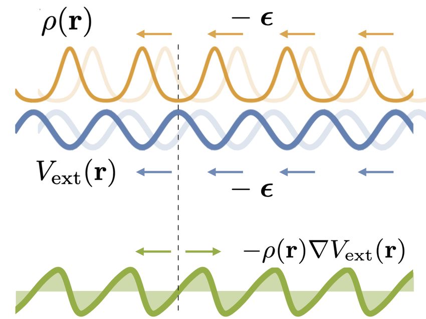
2

As soon as one is willing to accept this notion, making         scale of his entire body, but also when locally resolving
much headway is possible by analyzing physical proper-          his structure on the molecular scale.
ties of the considered system from this formal point of            In addition to shifting, one can also consider rotations.
view.                                                           In case of the action functional being invariant under ro-
   To perform the transfer and use Noether’s theorem for        tations Noether’s theorem implies that the angular mo-
thermal systems, from a formal point of view one would          mentum around the rotation axis is conserved. If the
need both to identify a suitable functional as well as a        free energy has rotational symmetry, fundamental state-
symmetry transformation under which this functional is          ments about torques emerge [14, 15]. These sum rules
invariant. One primary candidate for the choice of the          express inherent coupling of spin and orbital degrees of
functional is the partition function, which constitutes an      freedom. Figuratively speaking, the identities state that
integral over the high-dimensional phase space of classical     a bolt cannot screw itself into the wall and that a Baron
mechanics. Within this context, phase space describes all       Munchausen stuck in mud cannot spontaneously start to
degrees of freedom, i.e. the positions and momenta of all       rotate by twisting his head.
particles in the system. The partition sum itself is hence         Recognizing the functional dependence of the free en-
an integral over all these variables. Its integrand is, up to   ergy allows to build a theory fully founded on a vari-
a constant, the Boltzmann factor of the energy function         ational principle of thermal systems, as formulated by
that characterizes the system. So the partition sum ac-         Mermin [10] and Evans [11, 12]. Their so-called density
tually complies with the nature of a functional as it maps      functional theory is a well-accepted and widely used the-
this function to just a number, i.e. the value of the par-      ory, see Ref. [13] for a textbook presentation and Ref. [16]
tition sum. (As detailed below the interesting functional       for an overview of recent work. Excellent approximations
dependence is that on the external potential.) The parti-       are available for relevant model fluids, such as for hard
tion sum is arguably the most fundamental object in Sta-        spheres [17, 18] (see Ref. [19] for recent work addressing
tistical Physics, as all thermodynamic quantities, such as      hard sphere crystal properties). The density functional
thermodynamic potentials including the free energy, the         approach hence allows explicit calculations to be carried
equation of state, but also position-resolved correlation       out to predict the behavior of a wide range of physical
functions can be obtained from it, at least in principle.       systems, including solvation [20], hydrophobicity [21–23],
   Within Statistical Mechanics, where one identifies the       critical drying of liquids [24], solvent fluctuations [25],
free energy with the negative logarithm of the partition        electrolyte solutions near surfaces [26], interpretation of
sum, ordinary (parametric) derivatives of the free energy       atomic force microscopy data [27], temperature gradients
with respect to e.g. temperature and other thermody-            at fluid interfaces [28], and local fluctuations [22–25, 29].
namic variables generate thermodynamic quantities [11–          In Ref. [14] we also apply Noether’s thinking to a very
13]. While the familiar process of building the deriva-         recent variational approach for dynamics, called power
tive of a function, as giving a measure of the local slope,     functional theory [30, 31], which propels the functional
is a concept that dates back to Newton and Leibniz,             concepts from equilibrium to nonequilibrium [30–45], in-
functional differentiation is slightly less common. How-        cluding the recently popular active Brownian particles
ever, functionals can be differentiated in much the same        [46–52]. The generalization is important, as it shows that
way that functions can be differentiated. In case of the        not only a dead Munchausen cannot bootstrap himself
free energy, functional derivatives give microscopically        out of his misery, but that being alive does not help (in
resolved correlation functions [11–13]. These are quan-         this particular case).
tities, such as the structure factor of a liquid, that are         In the present contribution we demonstrate that the
measurable in a lab, say with a scattering apparatus or         concepts of Ref. [14] apply to the canonical ensemble,
even with a microscope upon further data processing.            as is relevant for confined systems [53–55] and for the
   When applying Emmy Noether’s thinking to the free            dynamics [56–58]. Hence having an open system with
energy, one could expect mere abstraction to result, but        respect to particle exchange is not necessary for the
that is not the case [14]. Consider the invariance under        Noetherian arguments to apply. We give a detailed and
a spatial shift. This classical application of Noether’s        somewhat pedagogical derivation of the fundamental con-
theorem to the action functional yields the well-known          cepts and also make much relevant background explicit,
result of momentum conservation. When rather exploit-           which has not been spelled out in Ref. [14].
ing the invariance of the partition function and hence             The paper is organized as follows. In Sec. II we go into
of the free energy with respect to shifting, what follows       some detail and we present in the following the arguably
are fundamental statements about forces that act in the         simplest example of the application of Noether’s Theo-
system [14]. One of them states that the total internal         rem to Statistical Mechanics. We expect the reader to be
force vanishes. Here the total internal force is that which     familiar with Newtonian mechanics and to ideally know
arises from the interactions only between the constituents      about Classical Mechanics formulated in a more formal
of the system. The famous Baron Munchausen tale of              setting (we supply some basic notions thereof below). We
bootstrapping himself out of the swamp by pulling on            lay out the canonical ensemble and averages in Sec. II A.
his own hair is identified as a fairytale by the Noetherian     Forces and their relation to symmetries are addressed in
argument. The impossibility of this feat holds on the           Sec. II B. Statistical functionals and their invariances are
3

described in Sec. II C. As an example we describe the               result from the above formulated microscopic picture.
application to sedimentation in Ref. II D. The relation-            Statistical Mechanics provides the means for doing so.
ship of the Noether invariance to correlation functions is          We will not attempt to give a comprehensive description
laid out in Sec. II E. We give further background that              of the concepts of this theory. Rather we will guide the
is relevant for Ref. [14], such as the details of the grand         reader through some essential steps, including in particu-
canonical treatment and the variational principles of den-          lar how thermal averages are built, to see how Noether’s
sity functional theory and of power functional theory, in           Theorem applies in this context. As we will see, both
Sec. II F. We present our conclusions in Sec. III.                  the physical concept and the outcome are different from
                                                                    the standard application of Noether’s theorem based on
                                                                    the action expressed as a time integral over a Lagrangian
                       II.     THEORY                               that corresponds to (1).
                                                                       Statistical Mechanics rests on the concept of having
         A.   Canonical ensemble and averages                       a statistical ensemble, in the sense of the collection of
                                                                    microstates r1 , . . . , rN , p1 , . . . , pN , i.e. all phase space
   We consider a system with fixed number of particles N .          points. These are transcended beyond Classical Mechan-
The state of the system is characterized by all positions           ics by each being assigned a probability for its occur-
r1 , . . . , rN and momenta p1 , . . . , pN , where the subscript   rence. (There is much discussion about who throws the
labels the N particles, which we take to all have identical         dice here; we recommend Zwanzig’s cool-headed account
properties. We assume that the total energy consists of             [59].) The microstate probability distribution is given by
kinetic and potential energy contribution, according to             a standard Boltzmann form,

           N
              p2i
                                           N                                                                              e−βH
                                                                                Ψ(r1 , . . . , rN , p1 , . . . , pN ) =        ,    (5)
          X                               X
       H=         + u(r1 , . . . , rN ) +     Vext (ri ).    (1)                                                           ZN
          i=1
              2m                          i=1
                                                                    where the inverse temperature is β = 1/(kB T ), with
Here H is the Hamiltonian of the system, with the inter-
                                                                    the Boltzmann constant kB and absolute temperature T .
particle interaction potential u(r1 , . . . , rN ) and the ex-
                                                                    Here ZN is the partition sum, and it acts to normalize the
ternal one-body potential Vext (ri ) acting on particle i.
                                                                    probability distribution to unity, when summed up over
The equations of motion are generated via ṙi = ∂H/∂pi
                                                                    all microstates. The sum over microstates is in practice
and ṗi = −∂H/∂ri , where the overdot indicates a time
                                                                    a high-dimensional integral over phase space, explicitly
derivative, m is the particle mass, and the index i =
                                                                    given as
1, . . . , N . Using the explicit form (1) of the Hamiltonian
then leads to the equations of motion in the familiar form                        1
                                                                                       Z
                                                                         ZN =             dr1 . . . drN dp1 . . . dpN e−βH , (6)
                                   pi                                          N !h3N
                             ṙi =      ,                    (2)
                                   m
                                                                    where h indicates the Planck constant. Here each posi-
                             ṗi = fi ,                      (3)
                                                                    tion integral and each momentum integral runs over R3 .
where fi indicates the force on particle i, which consists          (We are considering systems in three spatial dimensions.)
of a contribution from all other particles as well as the           The system volume is rendered finite by confining walls
external force. Explicitly, the force on particle i is given        that are modelled by a suitable form of the external po-
by                                                                  tential Vext (r). As a note on units, recall that h carries
                                                                    energy multiplied by time, i.e. Js, such that the partition
           fi = −∇i u(r1 , . . . , rN ) − ∇i Vext (ri ),     (4)    sum (6) carries no units.
                                                                       The purpose of the probability distribution (5) is to
where ∇i denotes the derivative with respect to ri .                build averages. Taking the Hamiltonian (1) as an exam-
(Building the derivative by a vector implies building the           ple, we can express the total energy, averaged over the
derivative with respect to each component of the vector,            statistical ensemble, as
hence ∇i can be viewed as building the gradient with re-                                  Z
spect to ri .) Certainly we could have written down the                               1
                                                                             E=              dr1 . . . rN dp1 . . . dpN HΨ. (7)
equations of motion (2) and (3) a priori. Equation (2)                             N !h3N
expresses the standard relation of velocity ṙi with mo-
mentum pi , and (3) is Newton’s second law. Hence we                Here we recall the dependence of the Hamiltonian (1) on
have reproduced the Newtonian theory within the Hamil-              the phase space point, and in the notation we have left
tonian formalism.                                                   away the arguments r1 . . . , rN , p1 , . . . , pN of both Ψ and
  So far everything has been deterministic and we were              H.
concerned with obtaining a description on the level of in-            It is useful to introduce more compact notation, as this
dividual particles. As our aim is to describe very large            reduces clutter and allows to express the structure of the
systems, we wish to “zoom out” and investigate and de-              theory more clearly. Let us denote the integral over phase
scribe the macroscopic properties of the system, as they            space, together with its normalizing factor in (6) as the
4
“classical trace” operation, hence defined as the occurrence of each given microstate. Hence the aver-
Z age total external force is given by
1
TrN = dr1 . . . drN dp1 . . . dpN , (8) N
N !h3N X
Ftot
ext = −TrN Ψ ∇i Vext (ri ). (12)
which is to be understood as acting on an integrand, such i=1
as on HΨ in the example (7) above. Equation (7) can Due to the structure of (12), Ftot
ext depends on the number
hence be expressed much more succinctly as of particles N (via the upper limit of the sum and the
dimensionality of the phase space integrals), on temper-
E = TrN HΨ. (9) ature T (via the thermal distribution Ψ, cf. (5) and (6)),
and it of course also depends on the form of the function
In a similar way we can express other averaged quantities,
Vext (r). Note that the function Vext (r) appears both ex-
such as the average external (potential) energy,
plicitly in the gradient in (12) as well as in a more hidden
N form in the probability distribution Ψ, cf. (5) and (1).
Let us halt for a moment and ponder the physics.
X
Uext = TrN Ψ Vext (ri ). (10)
i=1
Imagine having a vessel with impenetrable walls, such
that the system stays confined inside of the vessel. Fur-
In order to build some trust for the compact notation, thermore, to add some flavour, imagine an external field
we use (5) and (8) to re-write (10) explicitly as such as gravity acting on the system. Then the external
Z potential consists of two contributions, i.e. the poten-
1 tial energy that the container walls exert on each given
Uext = dr1 . . . drN dp1 . . . dpN
N !h3N particle plus the gravitational energy. In an equilibrium
N situation, what would we expect the total external force
e−βH X to be like? Surely, it should not change in time. (Tech-
× Vext (ri ), (11)
ZN i=1 nically any time evolution had been superseded by the
ensemble, which is a static one in the present case.) The
which allows to see explicitly that Uext depends on the reader might expect that
number of particle N and on the temperature T (via the
Boltzmann factor and the partition sum). Surely (10) al- Ftot
ext = 0, (13)
lows to see the physical content, that of an average being because otherwise the system would surely start to move!
carried out, more clearly than (11) and we will continue However, as for any given microstate the total external
to use the compact notation. (Readers who wish to fa- force will in general not vanish, (13), if true, is a non-
miliarize themselves more intimately with these benefits trivial property of thermal equilibrium. See Fig. 1 for
are encouraged to put pen to scratch paper and re-write an illustration. Hence we wish to address carefully in the
the following material in explicit notation.) following whether we can prove (13) from first principles.
We give two derivations of (13), which both rest on
spatial translations of the system. The first derivation
B. Forces and symmetries only requires vector calculus. We then proceed and show
the Noetherian symmetry argument based on the func-
Before continuing with thermal concepts, such as the tional setting. This requires to adopt the notion of func-
free energy, we take a detour from standard paths in Sta- tional dependencies, which we have used only implic-
tistical Mechanics, and return to forces. –After all, it was itly so far. In the following we make these relationships
the microscopically and particle-resolved forces fi in (4) and dependencies explicit. We also supply the neces-
that formed the starting point for the description of the sary methodology of functional differentiation and will
coupled system. As an example, let us hence consider attempt to convince the reader that their background in
the total external force that acts on the system, in the ordinary calculus can be flexed in order to follows these
sense that we sum up the external force that acts on each steps.
P particle, −∇i Vext (ri ). This accounting results
individual The fundamental ingredients to both derivations are
in − i ∇i Vext (ri ). Note that this expression still ap- identical though. We use the free energy and we moni-
plies per microstate, or in other words, the total external tor its changes upon spatial displacement of the system.
force varies in general across phase space. As a caution- The free energy, and more generally thermodynamic po-
ary note on terminology, we use throughout the term tentials, are central to thermal physics, and the following
“total” in the above sense of denoting a global, macro- material can be viewed as a demonstration why this in-
scopic, extensive quantity. This usage is different from deed is the case.
the also frequent meaning of total referring to the sum of The free energy FN , or more precisely: the total
intrinsic and external contributions. Helmholtz free energy is given by
In order to obtain the macroscopic description we need
to trace over phase space and respect the probability for FN = −kB T ln ZN , (14)5
choice of origin of the coordinate system does not mat-
ter). We can see this explicitly by performing a coor-
dinate transformation ri → ri − . This leaves Hint in-
variant, as the momenta are unaffected and the internal
interaction potential is unaffected. –Recall that the in-
terparticle energy only depends on relative particle posi-
tions, which remain invariant under the transformation:
ri − rj → (ri − ) − (rj − ) = ri − rj . Furthermore,
due to the simplicity of the coordinate transformation
that the shift represents, the phase space integral, cf. the
classical trace (8), is unaffected as the Jacobian of the
FIG. 1. Three representative microstates rN for N = 3 transformation is unity. Note that in the shifting oper-
particles inside of a spherical cavity modelled by a confin- ation, the momenta are unaffected and their behaviour
ing external potential Vext (r) (orange). Shown are the parti- remains governed by the Maxwell distribution through-
cle positions ri (pink dots) and the respective external force out. Hence we have shown that the original free energy
−∇i Vext (ri ) acting on particle i (black arrows). The result- is identical to the free energy of the shifted system
ing total external force F̂tot
P
ext = − i
∇ i Vext (ri ) is shown for
each microstate (blue arrows and blue dot, the later indi- FN = FN (), (19)
cating zero). Although F̂totext for each microstate is in gen-
eral nonzero, the average over the thermal ensemble vanishes, for any value of the displacement vector .
Ftot ext
ext = hF̂tot i = 0.
At this point one could conclude mission accomplished.
This is not what Emmy Noether did in her mathematical
formulation of the problem – we hint at her variational
where ZN is the partition sum, as defined in (6). One can techniques below. The way forward at this point is to
show that the relation of free energy and internal energy rather ignore (19) and return to the explicit expression
is given by the thermodynamic identity FN = E − T S, (17) for the free energy in the shifted system. We consider
where S is the entropy, here defined on a microscopic small displacements and Taylor expand to first order,
basis and the internal energy E is given by (9). One can
∂FN ()
surely be surprised by the promotion of the rather banal FN () = FN + · , (20)
normalization factor ZN to such a prominent and as we ∂ =0
show decisive role. We demonstrate in the following that where quadratic and higher order terms in have been
ZN had been a dark horse, and that its status to generate omitted. The partial derivative in (20) can be calculated
the free energy via (14) is well-deserved. explicitly:
Besides the free energy, the second ingredient that we
require is a spatial shift of the entire system according to ∂FN () kB T ∂
=− ZN () (21)
a displacement vector of the system. We hence displace ∂ ZN () ∂
the external potential spatially by a constant vector . kB T ∂
The displaced system is then under the influence of an =− TrN e−βH() (22)
ZN () ∂
external potential which has changed according to N
kB T ∂ X
Vext (r) → Vext (r + ). (15) =− TrN e−βH() (−β) Vext (ri − ),
ZN () ∂ i=1
Formally, the free energy of the displaced system will (23)
depend on the displacement vector, i.e.
where in the first step (21) the partition sum in the de-
FN → FN (), (16) nominator arises from the derivative of the logarithm in
(17) and in the second step (22) we have interchanged
where the new free energy is given by the phase space integration [as notated by TrN , cf. (8)]
and the -derivative. The third step (23) follows directly
FN () = −kB T ln ZN (). (17) from the structure of the Hamiltonian (1) and the fact
that Hint is independent of . We continue to obtain
Here the partition sum of the shifted system is
N
h X i ∂FN () e−βH() X ∂
ZN () = TrN exp − β Hint + Vext (ri + ) , (18) = TrN Vext (ri − ) (24)
∂ ZN () i=1 ∂
i
N
where the intrinsic part Hint of the Hamiltonian consists X ∂
= −TrN Ψ() Vext (ri − ), (25)
of kinetic energy and interparticle interaction potential ∂r i
i=1
energy only, i.e. Hint = i p2i /(2m) + u(r1 , . . . , rN ).
P
We proceed by first recognizing that the shift does not where in (24) we have pulled the partition sum as a con-
change the value of the free energy (in other words, the stant inside of phase space integral and have moved the6
-derivative inside the sum over all particles. In (25) introduction, integrals often allow for direct interpreta-
we have combined the Boltzmann factor with the par- tion as functionals as they map their integrand (or part
tition sum in order to express the many-body probabil- thereof) to the value of the quadrature. In the specific
ity distribution function in the shifted system, Ψ() = case at hand, we stay with the canonical free energy FN
exp(−βH())/ZN (), in generalization of (5). Further- and observe that its value certainly depends on the form
more the spatial derivative of the external potential is of the external potential Vext (r), cf. its occurrence in the
re-written via using ∂/∂ = −∂/∂ri (which is valid due Hamiltonian (1), which via the partition sum (6) enters
to the dependence on only the difference ri − ). Consid- the free energy (14). Hence we have FN [Vext ], where we
ering the case = 0 allows us to conclude that indicate the functional dependence by square brackets
(and leave away in the notation the position argument r,
N despite the fact that the functional depends on the en-
∂FN () X ∂
= −TrN Ψ Vext (ri ). (26) tire function). In order to highlight this point of view,
∂ =0
i=1
∂ri
we rewrite (14) and (6), respectively, in the form
Remarkably the right hand side is the average total ex-
ternal force as previously defined in (12). The left hand FN [Vext ] = −kB T ln ZN [Vext ], (28)
side is identically zero, as is arbitrary in (20) and the N
X
linear order (as well as all higher orders) need to vanish ZN [Vext ] = TrN exp − βHint − β Vext (ri ) , (29)
in the Taylor expansion (20) by virtue of the invariance i=1
(19) of the free energy upon spatial displacement. Hence
N
where still the partition sum, viewed now as a functional
X ∂ of the external potential, ZN [Vext ] is given by its elemen-
−TrN Ψ Vext (ri ) = 0, (27)
i=1
∂r i tary form, i.e. the right hand side of (6). In a more com-
pact form, eliminating ZN [Vext ] as a standalone object,
which proves constructively the anticipated vanishing we have
(13) of the average total external force (12).
As a preliminary summary, we have shown that the FN [Vext ] = (30)
invariance of a global thermodynamic potential, the
N
Helmholtz free energy expressed in the canonical ensem- X
− kB T ln TrN exp − βHint − β Vext (ri ) .
ble, against spatial displacement (as generated by a shift
i=1
of the external potential) leads to the non-trivial force
identity of vanishing total external force. This identity
holds true for any value of the number of particles in the We dwell on the functional concept and demonstrate
system, at arbitrary temperature, and most notably ir- some practical consequences. As an analogy, viewing the
respective of the precise form of the external potential. functional dependence in (30) akin to the dependence of
Hence we refer to statements such as Ftot ext = 0, cf. (13),
an ordinary function f (x) on its argument x brings con-
as a Noether identity or Noether sum rule. Clearly the cepts of calculus immediately to mind, such as building
concept is general, as both the symmetry operation can the derivative f 0 (x) and investigating its properties.
be altered (rotations are considered in Ref. [14]) as well This analogy extends to functionals and their deriva-
as the type of thermodynamic object can be changed (the tives with respect to the argument function, in a pro-
grand potential and the excess free energy density func- cess referred to as functional differentiation. For the
tional are considered in Ref. [14] and we shift the total present case, functionally deriving Fext [Vext ] with respect
external energy Uext below in Sec. II E). to Vext (r) can be viewed as monitoring the change of the
We have presented here the shifting from the point of value of the functional upon changing its argument func-
view that the actual physical system is moved to a differ- tion at position r. The change will in general depend
ent location. Alternatively, one could adopt a “passive” on position r, hence building functional derivatives cre-
point of view and displace only the origin of the coor- ates position dependence. (The result of the functional
dinate system, in the sense of using shifted coordinates derivative is again a functional, as the dependence on
that still describe an unchanged physical system. Then the argument function persists.) Functional calculus is
going through a chain of arguments analog to those given in many ways similar to ordinary multi-variable calculus.
above yields identical results. We do not attempt to give a tutorial here (see e.g. the
appendix of Ref. [31] for a very brief one), but rather
present a single example that is relevant for the present
C. Functionals and invariances physics of invariance operations applied to many-body
systems.
The abstraction that is yet to be performed and that We use standard notation and denote the func-
allows to see the above result in an even wider setting, is tional derivative with respect to the function Vext (r) as
based on functional methods. As we had hinted at in the δ/δVext (r). Applying this procedure to the free energy7
(28) yields
δFN [Vext ] δ
= −kB T ln ZN [Vext ] (31)
δVext (r) δVext (r)
kB T δ
=− ZN [Vext ], (32)
ZN [Vext ] δVext (r)
where in the first step we have taken the multiplicative
constant −kB T out of the derivative and in the second
step have used the ordinary chain rule, which also holds
for functional differentiation. We next use the explicit
form (29) to obtain
δFN [Vext ] kB T δ
=− TrN e−βH (33)
δVext (r) ZN [Vext ] δVext (r)
kB T δ
=− TrN e−βH (−βH) (34)
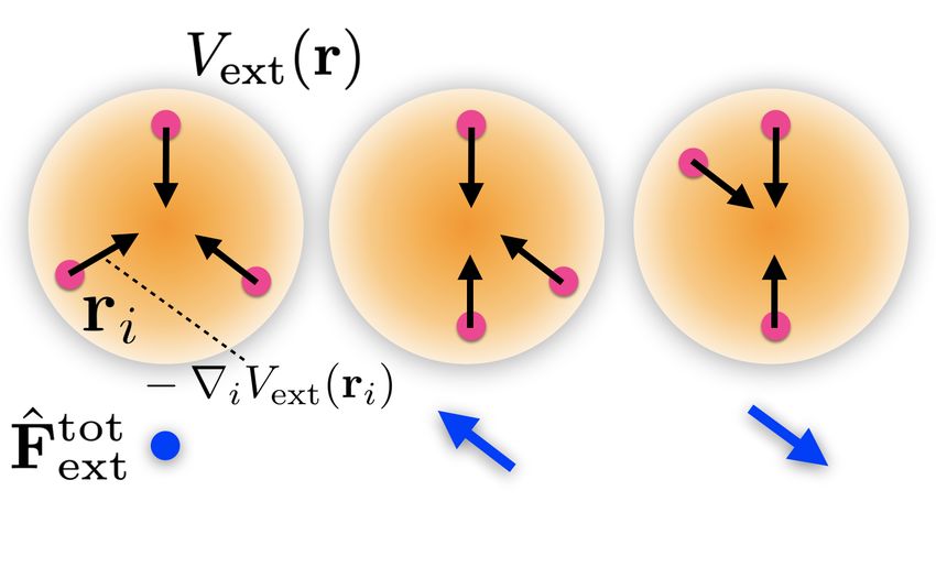
ZN [Vext ] δVext (r) FIG. 2. Illustration of the shifting. A sinusoidal external po-
N tential Vext (r) (blue lines) is spatially displaced by a displace-
1 δ X
= TrN e−βH Vext (ri ), ment − (blue arrows). The density profile ρ(r) (amber lines)
ZN [Vext ] δVext (r) i=1
measures the local probability to find a particle; it hence has
(35) e.g. peaks at the troughs of the external potential and it is
shifted accordingly (amber arrows). Also shown is the magni-
where we have first exchanged the order of the functional tude of the external force density −ρ(r)∇Vext (r) (green line);
the green arrows represent its local direction. The horizontal
derivative and the phase space integral, i.e. moved the
dashed line is a guide that indicates the position of locally
derivative inside of the trace in (33), then in the sec- vanishing external force density.
ond step (34) have used the chain rule to differentiate
the exponential, and in the last step (35) have exploited
the structure (1) of the Hamiltonian. Moving the deriva- spatial shifting. Recall the elementary Taylor expansion
tive inside of the sum over i and identifying the many-
body probability distribution function Ψ according to (5) Vext (r + ) = Vext (r) + · ∇Vext (r), (37)
yields the final result
where ∇ indicates the derivative (gradient) with respect
δFN [Vext ] X
to r and we have truncated at linear order. See Fig. 2
= TrN Ψ δ(r − ri ) ≡ ρ(r), (36)
δVext (r) i for an illustration. The first order term in (37) can
be viewed as a local change in the external potential,
where we have used one central rule of functional dif- δVext (r), which is given by
ferentiation: differentiating a function by itself gives
δVext (ri )/δVext (r) = δ(r − ri ), where the result δ(·) is δVext (r) ≡ · ∇Vext (r). (38)
the Dirac delta distribution (here in three dimensions, as
its argument is a three-dimensional vector). In order to capture the resulting effect on the func-
Notably in (36) we have arrived at the form of a tional, we can functionally Taylor expand the dependence
thermal average over the statistical ensemble; recall the of the free energy on Vext (r) + δVext (r) around the func-
generic form exemplified by the average internal en- tion Vext (r). To linear order in δVext (r) the functional
ergy (9). Rather than the expectation value of the Hamil- Taylor expansion reads
tonian, the present case represents the average of the mi- Z
PN δFN [Vext ]
croscopically resolved density operator i=1 δ(r − ri ), FN [Vext + δVext ] = FN [Vext ] + dr δVext (r)
which can be viewed as an indicator function that mea- δVext (r)
sures whether any particle resides at the given position r. (39)
Z
The result of the average is the one-body density distribu-
= FN [Vext ] + drρ(r) · ∇Vext (r),
tion, or in short the density profile ρ(r). That functional
differentiation yields useful, spatially-resolved (“correla- (40)
tion”) functions is a general mechanism. See e.g. [13]
for much background on correlation functions and their where in (40) we have used the explicit form (38) of
generation via functional differentiation. Reference [14] δVext (r) as it arises from the fact that the variation in
carries this concept much further than we do here. the shape of the external potential is specifically gener-
We return to the shifting symmetry operation of above, ated by a spatial displacement, cf. (37). Furthermore
but now monitor the system response via tracking the we have used (36) to identify the functional derivative in
changes in the function Vext (r) that are induced by the (39) as the density profile.8
The result (40) is based on the properties of functional Vext → ∞ for z → ∞. The magnitude of the external
0
calculus alone. Hence the identity is general and holds, force field is obtained as −Vext (z) = −mg − αzΘ(−z),
to linear order in , irrespective of any invariance prop- see Fig. 3 for an illustration (blue line).
erties. For the case of the total free energy, which as The density distribution of the isothermal ideal gas is
we have shown above in (19) is invariant under spatial given by the generalized barometric law [13],
displacement, we have
ρ(z) = Λ−3 e−β(Vext (z)−µ) , (45)
FN [Vext ] = FN [Vext + δVext ], (41)
where Λ is the thermal de Broglie wavelength which arises
where δVext (r) is generated from the spatial displacement from carrying out the momentum integrals in TrN (this
of the system, cf. (38). Hence (38) together with (41) ex- is analytically possible due to the simple kinetic energy
press in functional language the translational symmetry part of the Boltzmann factor). The chemical potential µ
properties of the free energy. in (45)R is a constant that ensures the correct normaliza-
From the identity (41) and the linear Taylor expansion tion, dzρ(z) = N/A, where A is the lateral system size
(40) we can conclude that the correction term needs to (i.e. the area perpendicular to the z-direction). That the
vanish, value of the chemical potential µ controls the number of
Z particles in the system is universal. However, the math-
ematical formulation in the grand ensemble, where the
drρ(r) · ∇Vext (r) = 0. (42)
particle number in the system can fluctuate, is very differ-
ent from the present canonical treatment. (Some basics
The displacement vector is arbitrary, as there was no of the grand canonical description, as used in Ref. [14],
restriction on the direction of the shift. Hence the above are described below in Sec. II F.)
expression can only identically vanish provided that The general expression for the total external force (43)
Z together with the specific density profile (45) gives
tot
Fext = − drρ(r)∇Vext (r) = 0, (43)
Aez ∞
Z
Ftot
ext = − dze−β(Vext (z)−µ) Vext
0
(z) (46)
Λ3 −∞
where we have multiplied by −1 in order to identify the i∞
one-body expression for the total external force Ftot Aez h
ext ; the = 3 e−β(Vext (z)−µ) (47)
equivalence with the many-body form (12) is straight- Λ β −∞
forward to show upon using the definition of the density = 0, (48)
profile (36). See Fig. 2 for an illustration of the local
force density profile, i.e. the integrand of (43). where ez is the unit vector pointing into the positive z-
direction and the prime denotes differentiation with re-
0
spect to the argument, hence ∇Vext (r) = Vext (z)ez . The
−β(Vext −µ)
D. Application to sedimentation integrand in (46) is a total differential, de /dz,
which upon integration gives (47); for (48) we have ex-
We exemplify the general result (43) using the con- ploited that for z → ±∞ the external potential Vext →
crete example of a thermal system under gravity, such ∞, leading to vanishing Boltzmann factor. We have
that sedimentation-diffusion equilibrium is reached. Re- hence shown explicitly the vanishing of the total exter-
call that we consider systems at finite temperature, where nal force acting on a bounded ideal gas in thermal equi-
entropic effects compete with ordering generated by the librium under gravity. Figure 3 illustrates the density
0
potential energy. We first omit the interparticle interac- profile ρ(z) and the force density profile −Vext (z)ρ(z) for
tions, and hence consider the classical monatomic ideal representative values of the parameters.
gas. We assume that the external potential consists of We briefly sketch the effect of interparticle interactions.
a gravitational contribution, mgz, where g indicates the On a formal level, and returning to the general case of
gravitational acceleration and z is the height variable. arbitrary form of Vext (r), the density profile is given by
Furthermore due to the presence of a lower container a modified form of (45), which reads
wall, there is a repulsive contribution, which we take to
be a harmonic potential with spring constant α acting ρ(r) = Λ−3 e−β(Vext (r)−µ)+c1 (r) , (49)
“inside” the wall, i.e. at altitudes z < 0. Hence the spe- where the so-called one-body direct correlation function
cific form of the total external potential is [11, 13] c1 (r) contains the effects of the interparticle in-
teractions. The total interparticle force density is then
αz 2
Vext (z) = mgz + Θ(−z), (44) given by
2 Z
tot
where Θ(·) indicates the Heaviside (unit step) function, Fint = kB T drρ(r)∇c1 (r) = 0. (50)
which ensures that the parabolic potential only acts for
z < 0. There is no need for the presence of an upper wall Here the vanishing of the total internal force can be
to close the system, as gravity alone already ensures that viewed as a consequence of Newtons’ third law actio9
fer the reader to Ref. [14] for this treatment, we wish
to demonstrate here the direct derivation of such global
identities.
We stick to the canonical ensemble and as a specific
case return to our initial example of a thermal average,
i.e. the global external potential energy Uext , as equiva-
lently expressed in compact notation (10) or the explic-
itly written out phase space integral (11). Let us shift!
The external energy in the new system is then given by
N
e−βH() X
Uext () = TrN Vext (ri − ). (51)
ZN () i=1
We Taylor expand to first order,
∂Uext ()
Uext () = Uext + · . (52)
∂ =0
Here the derivative of (51) can be calculated via the prod-
uct rule as
N
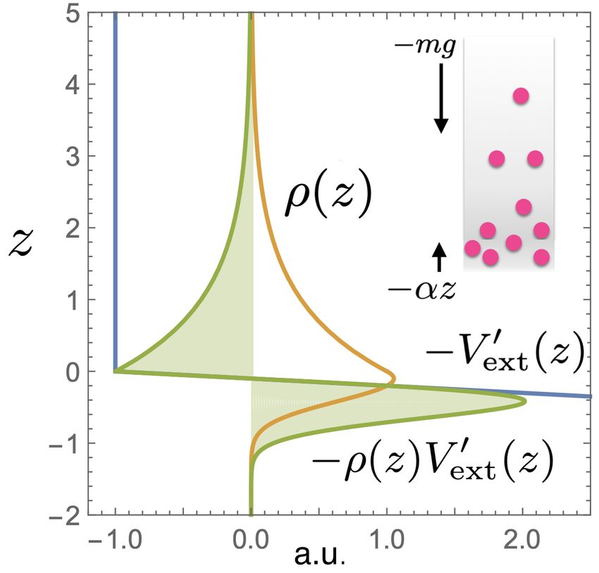
FIG. 3. Illustration of sedimentation of a fluid against a lower ∂Uext () ∂Ψ() X
= Tr Vext (ri )
soft wall represented by a harmonic potential. The total ex- ∂ =0 ∂ i=1
ternal potential is Vext (z) = mgz + Θ(−z)αz 2 /2. The re-
0 N
sulting external force field is −Vext (z) ≡ −∂Vext (z)/∂z = X
−mg − Θ(−z)αz (blue line). The direction of both force − Tr Ψ ∇i Vext (ri ). (53)
contributions is indicated in the inset (arrows), where pink i=1
dots represent particles. In the main plot the density pro- We can recognize the second term as the average external
file ρ(z) (amber line) decays for large and for small values force, which we have proven to vanish, cf. (27). The first
0
of z. The external force density is the product −ρ(z)Vext (z) term in (53) requires carrying out the derivative of Ψ()
(green line). The total external force (per unit area) is the with respect to the displacement , which yields
0
R
integral − dzVext (z)ρ(z) = 0; note that the shaded green
areas cancel each other. Representative values of the parame- N N
∂Uext () X X
ters are chosen; the unit of length is the sedimentation length = −Tr Ψ βVext (ri ) ∇j Vext (rj ).
kB T /(mg) and all energies are scaled with kB T . ∂ =0
i=1 j=1
(54)
Here an additional term, generated by the derivative,
equals reactio; see Ref. [14] for the derivation. Note tot
vanishes: −βUext Fext = 0, again due to (27).
the formal similarity of the total external and total in-
Clearly (54) is the correlator of the global external po-
trinsic force Noether sum rules, cf. (43) and (50). The
tential energy and the global external force. Using the
no-bootstrap theorem (50) holds beyond equilibrium, as
by now familiar invariance argument, we argue that the
shown in Ref. [14], and it hence debunks any swamp es-
value of Uext () is an invariant under the displacement,
cape myths.
and that hence the first order term in (52) needs to be
An alternative derivation of (50) rests on the Noether
zero. As is arbitrary, we conclude
invariance of the free energy, where the later is con-
structed to be a functional of the density profile; we refer N
X N
X
the Reader to Ref. [14] for a description of these con- −Tr Ψ Vext (ri ) ∇j Vext (rj ) = 0, (55)
siderations and comment briefly on the embedding into i=1 j=1
the frameworks of classical density functional theory and where we havePdivided by β. Hence the global exter-
power functional theory below in Sec. II F. nalPpotential, i Vext (ri ), and the global external force,
− j ∇j Vext (rj ), are uncorrelated with each other. The
sum rule (55) is derived in Ref. [14] via the route of inte-
E. Relationship to correlation functions gration over free position variables (root points), cf. (5)
in Ref. [14] for the order n = 2 of the sum rule hierarchy.
Global identities, such as the sum rules of vanishing ex- An important distinction in the presentation though lies
ternal force (43) and of vanishing internal force (50), can in the choice of ensemble, which is an issue to which we
be used as a starting point to obtain position-resolved turn in the next subsection.
identities. Functional differentiation with respect to an As a final comment, when applied to the above exam-
appropriate field creates dependence on position. Inte- ple of sedimentation against a lower harmonic wall, (55)
grating over these additional variables (or “root points” can be explicitly Rverified by carrying out the z-integral,
∞ 0
[13]) then yields novel global identities. While we re- which yields −A ∞ dzρ(z)Vext (z)Vext (z) = 0.10
F. Density functional and power functional (57); the trace (8) with (58); and the free energy (14)
with (60).
In all of the above, we have described the thermal sys- Despite the system being open to particle exchange,
tem on the basis of the canonical ensemble, as specified Noether’s reasoning continues to hold [14]. Briefly, the
by the classical phase space, the probability distribution grand potential is a functional of the external potential,
(5) and the canonical partition sum (6). Hence the sys- Ω[Vext ] (we suppress the dependence on the thermody-
tem is coupled to a heat bath at temperature T , where namic parameters µ, T ), and Ω[Vext ] is invariant under
the value of T determines the mean energy E in the sys- spatial displacements according to (15). As a conse-
tem, cf. the form of E as an expectation value (7). The quence, the sum rule of vanishing external force (13)
system is thermally open, and hence energy fluctuations emerges, expressed in the form (27) with TrN replaced
occur between system and bath. by Tr, as is appropriate for the open system.
Corresponding fluctuations in particle number N can Why is the functional point of view important? In
be implemented in the grand canonical ensemble where what we have presented above it had played the role of
the system is furthermore coupled to a particle bath. The adding abstraction and re-deriving results that we could
particle bath sets the value of the chemical potential µ, obtain via more elementary arguments. The importance
which then determines the average number of particles of the variational formulation stems from two sources,
N̄ in the system. (This mechanism is analogous to the one being that it provides a mechanism for the gener-
relationship of T and E described above.) Although the ation of correlation functions via functional differentia-
grand canonical formalism poses this additional level of tion, in extension of the generation of the density profile
abstraction, and the bare formulae increase somewhat in via (36), see e.g. Refs. [13] for a comprehensive account.
complexity due to the average over N , in typical theo- The second point lies in the variational principle itself
retical developments this framework is significantly more which formulates the many-body problem in a way that
powerful and more straightforward to use. (There is no allows to systematically introduce approximations and
need having to implement N = const, which in practice make much headway in identifying and studying phys-
can be awkward.) We briefly sketch the essentials of the ical mechanisms in complex, coupled many-body prob-
grand ensemble as they underlie Ref. [14]. lems. While giving a self-contained overview of these
The grand canonical ensemble consists of the mi- concepts is beyond the scope of the present contribution
crostates given by phase space points of N particles, with (see Ref. [31] for a recent account), we wish to briefly
N being a non-negative integer, which is treated as a ran- describe certain central points, to –hopefully– provide
dom variable. The corresponding probability distribution motivation for further study.
is We hence sketch the two variational principles as they
are relevant for equilibrium (classical density functional
e−β(H−µN ) theory) and for the dynamics (power functional theory);
Ψ(r1 , . . . , rN , p1 , . . . , pN , N ) = , (56) these form the basis of Ref. [14]. Classical density func-
Ξ
tional theory is based on treating the density profile ρ(r),
where the grand partition sum is given by rather than the external potential Vext (r), as the fun-
damental variational field. The grand potential, when
Ξ = Tr e−β(H−µN ) , (57) viewed as a density functional [11, 12], has the form
with the grand canonical trace operation defined by Z
Ω[ρ] = F [ρ] + drρ(r)(Vext (r) − µ), (61)
∞
X
Tr = TrN (58)
N =0
where F [ρ] is the intrinsic Helmholtz free energy func-
∞ Z tional. Crucially, F [ρ] is independent of the external po-
X 1 tential, which features solely in the second term in (61).
= dr1 . . . drN dp1 . . . dpN , (59)
h3N N ! Here ρ(r) is conceptually treated as a variable; its true
N =0
form as the equilibrium density profile is that which min-
where we have obtained (59) by using the explicit form imizes Ω[ρ] and for which hence the functional derivative
(8) for the canonical trace. The thermodynamic potential vanishes,
which is fundamental for the grand ensemble is the grand
potential (also referred to as the grand canonical free δΩ[ρ]
=0 (min). (62)
energy) and it is given by δρ(r)
Ω = −kB T ln Ξ, (60) Inserting the split form (61) of the grand potential into
the minimization condition (62) and using the splitting
with the grand partition sum Ξ according to (57). Note into ideal gas and excessR (over ideal gas) free energy con-
the strong formal analogy with the corresponding canon- tributions, F [ρ] = kB T drρ(r)[ln(ρ(r)Λ3 ) − 1] + Fexc [ρ],
ical expressions for: the probability distribution (5) with yields upon exponentiating the Euler-Lagrange equation
(56); the partition sum (6), i.e. ZN = TrN e−βH , with in the modified barometric form (49). Here the one-body11
direct correlation function c1 (r) is identified as the func- via Fad (r, t) = −ρ(r, t)∇δF [ρ]/δρ(r, t) and an additional
tional derivative of the excess free energy functional, i.e. genuine nonequilibrium contribution, i.e. the superadia-
c1 (r) = −βδFexc [ρ]/δρ(r). As the functional dependence batic force density, Fsup (r, t). Honoring its functional de-
on the density profile persists upon building the deriva- pendence on the kinematic fields ρ(r, t) and J(r, t) forms
tive, i.e. in more explicit notation c1 (r, [ρ]), the Euler- the basis for much recent work in Nonequilibrium Statis-
Lagrange equation in the from (49) constitutes a self- tical Mechanics based on the power functional concept.
consistency condition for the determination of the equi-
librium density profile; determining the solution thereof
requires to have an approximation for Fexc [ρ] and typi- III. CONCLUSIONS
cally involves numerical work.
Power functional theory generalizes the variational
In conclusion, we have demonstrated on an elementary
concept of working on the level of one-body correlation
level how fundamental symmetries in Statisical Mechan-
functions to nonequilibrium. For overdamped Brownian
ics lead to exact statements (sum rules) about average
motion, as is a simple model for the description for the
forces when considering translations. These considera-
temporal behaviour of mesoscopic particles that are sus-
tions also apply to torques when considering rotations
pended in a liquid, the free power is a functional of both
[14]. We have based our presentation on the canonical
the time-dependent density profile ρ(r, t) and of the lo-
ensemble, as is relevant in a variety of contexts [53–58].
cally resolved current distribution J(r, t), where t indi-
While the canonical ensemble avoids the complexity of
cates time. The power functional has the form
particle number fluctuations that occur grand canoni-
Rt [ρ, J] = Ḟ [ρ] + Pt [ρ, J] (63) cally, nevertheless an open system is retained with re-
Z spect to energy exchange with a heat bath. As we have
− dr(J(r, t) · fext (r, t) − ρ(r, t)V̇ext (r, t)), shown, treating such fluctuating systems is well permissi-
ble on the basis of Noetherian arguments. The arguably
where Ḟ [ρ] is the time derivative of the intrinsic free en- simplest Noether sum rule is that of vanishing average
ergy functional, Pt [ρ, J] consists of an ideal gas and a su- total external force in thermal equilibrium. As an ap-
peradiabatic part, where the latter arises from the inter- plication we have presented the case of a fluid confined
nal interactions in the nonequilibrium situation, fext (r, t) inside of a container and subject to the effect of gravity.
is a time-dependent external one-body force field, which While we have selected this example for its relative sim-
in general consists of a (conservative) gradient term plicity, the influence of gravity on mesoscopic soft mat-
−∇Vext (r, t) and an additional rotational (non-gradient, ter is also a topic of relevance for studying e.g. complex
non-conservative) contribution, and V̇ext (r, t) is the time phase behaviour in colloidal mixtures; see e.g. Ref. [60]
derivative of the external potential. The density profile for recent work that addresses colloidal liquid crystals.
and the current distribution are linked by the continuity Our derivations imply that the symmetry operation is
equation, ∂ρ(r, t) = −∇·J(r, t), which is sharply resolved applied to the entire system. Here the system must be
on the microscopic scale. The dynamic variational prin- enclosed by an external potential that represents confine-
ciple states that Rt [ρ, J] is minimized, at time t, by the ment by e.g. walls. The shift then applies also to these
physically realized current, walls. In cases where system boundaries are open (as can
be suitable for a periodically repeated system like that
δRt [ρ, J] shown in Fig. 2), Noether’s theorem remains applicable
=0 (min). (64)
δJ(r, t) upon taking account of additional boundary terms, see
Ref. [14] for a detailed discussion of such treatment.
Inserting the splitting (63) of the total free power into Statistical mechanical derivations often rely on very
the minimization condition (64) yields an Euler-Lagrange similar reasoning; Ref. [14] gives an overview. A par-
equation which constitutes a formal exact force density ticularly insightful example is the work by Bryk et al.
relationship, on hard sphere fluids in contact with curved substrates
γJ(r, t) = −kB T ∇ρ(r, t) + Fint (r, t) + ρ(r, t)fext (r, t), [64]. These authors derive a contact sum rule of the hard
(65) sphere fluid against a hard curved wall. Their argumen-
tation rests on the observation that the force that is nec-
where γ is the friction constant of the overdamped mo- essary to move the wall by an amount is balanced by
tion, such that the left hand side constitutes the (nega- the presence of the fluid. The authors then succeed in
tive) friction force density at position r and time t. The relating this force to the value of the density profile close
right hand side of (65) consists of an ideal, an internal to the wall. Closely related work was carried out for the
and an external driving contribution, with Fint (r, t) be- shape dependence of free energies [65]. Further studies
ing the internal force density distribution, as it arises that are related to Noether’s Theorem were aimed at bro-
from the effect of all interparticle interactions that act ken symmetries [66] and emerging Goldstone modes [67–
on a given particle at position r and time t. The internal 69].
force density Fint (r, t) consists of an adiabatic contribu- The general form of Noether’s Theorem applies to vari-
tion, which follows from the excess free energy functional ational calculus, and Statistical Mechanics falls well into12
this realm. We have spelled out the connections explic- fulness has been amply demonstrated, both for formal
itly, such as the canonical free energy being viewed as a work as well as for practical solution of physical prob-
functional of the external potential [13]. Notably only lems and the discovery of novel fundamental mechanisms.
elementary statistical objects such as the partition sum The reformulation on the basis of the velocity gradient
are required. We have also described two more advanced [39], instead of the current distribution, allowed to iden-
variational theories. Classical density functional theory tify and to study structural forces [40, 41] in driven sys-
[11–13] allows to view the grand potential as a functional tems that are governed by overdamped Brownian dynam-
of the one-body density distribution. A formally exact ics. The splitting of the total internal force field into
minimization principle then reformulates the physics of flow and structural contributions is fundamental to un-
system in thermal (and chemical) equilibrium. The dy- derstanding the emerging effects in microscopically in-
namic variational principle of power functional theory homogeneous flows [41]. Active Brownian particles, as
[30, 31] consists of instantaneous minimization with re- a model for self-propelled colloids (see e.g. [46–48]), are
spect to the time- and position-resolved current distribu- well suited for the application of power functional the-
tion. Together with the continuity equation, a formally ory. The general framework [33, 34] for active systems
closed one-body reformulation of the dynamics of the un- was shown to physically explain and quantitatively pre-
derlying many-body system is achieved. dict the motility-induced phase separation that occurs in
Both density functional theory and power functional such systems at high enough levels of driving [35–37]. In-
theory can be viewed as systematic approaches to coarse- terfacial properties such as polarization [38] and surface
graining the many-body problem to the level of one-body tension [35] were systematically studied.
correlation functions. In the static case, the correlation The dynamical sum rules for forces and correlation
functions hence depend on position alone, in the dynam- functions presented in Ref. [14] offer great potential
ics case the dependence is on position and on time. Cru- for systematic progress in the description of complex
cially, a microscopically sharp description is formally re- temporal behaviour, including memory [44, 45]. The
tained, which is important for the description of corre- nonequilibrium rules play a similar role than fundamen-
lations on the particle (i.e. molecular or colloidal) level. tal equilibrium sum rules such e.g. the Lovett-Mou-Buff-
One of the most important features of these theories is Wertheim equation [70, 71]. The section on “Methods”
the identification of a universal intrinsic functional that in Ref. [14] gives a detailed description of the relationship
contains the coupled effects of the interparticle interac- of the equilibrium Noether sum rules to to such classical
tions, but is independent of the external forces that act results from the liquid state literature. Together with the
on the system. nonequilibrium Ornstein-Zernike relations [42, 43] the
A wealth of productive research have been devoted dynamical sum rules provide fertile ground for making
to constructing powerful approximations for free energy progress in nonequilibrium many-body physics. Hence
functionals for specific model systems. In the context the fundamental character of Emmy Noether’s work will
of liquids the important case of the hard sphere fluid is surely continue to prove its worth in the future.
treated with excellent accuracy within Rosenfeld’s fun-
damental measure theory [17, 18], see e.g. Ref. [61] for
a quantitative assessment of the quality of theoretical
density profiles against simulation data. Notable recent
progress to incorporate short-ranged attraction into den- ACKNOWLEDGMENTS
sity functional theory is due to Tschopp, Brader and their
coworkers [62, 63], who systematically addressed and ex- We thank Daniel de las Heras, Roland Roth, and Bob
ploited two-body correlations. Evans for useful comments and discussions. This work is
Despite power functional theory [30, 31] being signif- supported by the German Research Foundation (DFG)
icantly younger than density functional theory, its use- via project number 436306241.
[1] Invariante Variationsprobleme. E. Noether, Nachr. d. [3] N. Byers, “E. Noether’s discovery of the deep con-
König. Gesellsch. d. Wiss. zu Göttingen, Math.-Phys. nection between symmetries and conservation laws,”
Klasse, 235 (1918). English translation by M. A. Tavel: arXiv:physics/9807044 (1998).
Invariant variation problems. Transp. Theo. Stat. Phys. [4] A. G. Lezcano and A. C. M. de Oca, “A Stochastic Ver-
1, 186 (1971); for a version in modern typesetting see: sion of the Noether Theorem,” Found. Phys. 48, 726
Frank Y. Wang, arXiv:physics/0503066v3 (2018). (2018).
[2] For a description of many insightful and pedagogical [5] J. C. Baez and B. Fong, “A Noether theorem for Markov
examples and applications, see: D. E. Neuenschwan- processes,” J. Math. Phys. 54, 013301 (2013).
der, Emmy Noether’s Wonderful Theorem (Johns Hop- [6] I. Marvian and R. W. Spekkens, “Extending Noether’s
kins University Press, Baltimore, 2011). theorem by quantifying the asymmetry of quantum
states,” Nat. Commun. 5, 3821 (2014).You can also read