Transport of short-lived halocarbons to the stratosphere over the Pacific Ocean - Atmos. Chem. Phys
←
→
Page content transcription
If your browser does not render page correctly, please read the page content below
Atmos. Chem. Phys., 20, 1163–1181, 2020
https://doi.org/10.5194/acp-20-1163-2020
© Author(s) 2020. This work is distributed under
the Creative Commons Attribution 4.0 License.

Transport of short-lived halocarbons to the stratosphere over
the Pacific Ocean
Michal T. Filus1 , Elliot L. Atlas2 , Maria A. Navarro2,† , Elena Meneguz3 , David Thomson3 , Matthew J. Ashfold4 ,
Lucy J. Carpenter5 , Stephen J. Andrews5 , and Neil R. P. Harris6
1 Centre for Atmospheric Science, University of Cambridge, Cambridge, CB2 1EW, UK
2 Department  of Atmospheric Sciences, RSMAS, University of Miami, Miami, Florida, USA
3 Met Office, Atmospheric Dispersion Group, FitzRoy Road, Exeter, EX1 3PB, UK
4 School of Environmental and Geographical Sciences, University of Nottingham Malaysia, 43500,

Semenyih, Selangor, Malaysia
5 Wolfson Atmospheric Chemistry Laboratories, Department of Chemistry, University of York, York, YO10 5DD, UK
6 Centre for Environmental and Agricultural Informatics, Cranfield University, Cranfield, MK43 0AL, UK
† deceased

Correspondence: Neil R. P. Harris (neil.harris@cranfield.ac.uk)

Received: 26 June 2018 – Discussion started: 7 September 2018
Revised: 8 August 2019 – Accepted: 10 October 2019 – Published: 31 January 2020

Abstract. The effectiveness of transport of short-lived halo-      transport processes. Our results support recent estimates of
carbons to the upper troposphere and lower stratosphere re-        the contribution of short-lived bromocarbons to the strato-
mains an important uncertainty in quantifying the supply           spheric bromine budget.
of ozone-depleting substances to the stratosphere. In early
2014, a major field campaign in Guam in the western Pacific,
involving UK and US research aircraft, sampled the tropi-
cal troposphere and lower stratosphere. The resulting mea-
surements of CH3 I, CHBr3 and CH2 Br2 are compared here            1   Introduction
with calculations from a Lagrangian model. This methodol-
ogy benefits from an updated convection scheme that im-            The successful implementation of the Montreal Protocol with
proves simulation of the effect of deep convective motions         its adjustments and amendments has led to reductions in
on particle distribution within the tropical troposphere. We       stratospheric chlorine and bromine amounts since the late
find that the observed CH3 I, CHBr3 and CH2 Br2 mixing ra-         1990s (Carpenter et al., 2014). These reductions have halted
tios in the tropical tropopause layer (TTL) are consistent with    the ozone decrease (Harris et al., 2015; Chipperfield et al.,
those in the boundary layer when the new convection scheme         2017; Steinbrecht et al., 2017) with the exception of the pos-
is used to account for convective transport. More specifi-         sible reduction in the lower stratosphere (Ball et al., 2017,
cally, comparisons between modelled estimates and obser-           2019; Chipperfield et al., 2017). Recently, the importance
vations of short-lived CH3 I indicate that the updated convec-     of very short-lived (VSL) chlorine- and bromine-containing
tion scheme is realistic up to the lower TTL but is less good at   compounds has received a great deal of attention (e.g. Hos-
reproducing the small number of extreme convective events          saini et al., 2017; Oram et al., 2017). VSLs are not controlled
in the upper TTL. This study consolidates our understanding        under the Montreal Protocol but are required in order to rec-
of the transport of short-lived halocarbons to the upper tro-      oncile observed stratospheric measurements of inorganic or
posphere and lower stratosphere by using improved model            “active” bromine with reported anthropogenic bromine emis-
calculations to confirm consistency between observations in        sion sources. However, VSL input into the stratosphere has
the boundary layer, observations in the TTL and atmospheric        remained a poorly constrained quantity (Carpenter et al.,
                                                                   2014), which hinders our understanding of the ongoing de-

Published by Copernicus Publications on behalf of the European Geosciences Union.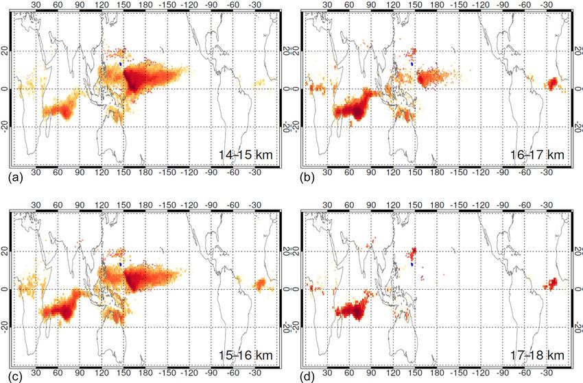
1164                    M. T. Filus et al.: Transport of short-lived halocarbons to the stratosphere over the Pacific Ocean

cline in lower stratospheric ozone and our ability to make          deep convection. This campaign produced a unique dataset of
predictions of stratospheric ozone recovery.                        coordinated measurements for interpretative studies of trans-
   Three of the most important VSL halocarbons are methyl           port and distribution of the chemical species, including the
iodide, CH3 I; bromoform, CHBr3 ; and dibromomethane,               VSL bromocarbons (Sect. 2.1 and 2.2). The NASA ATTREX
CH2 Br2 . They have typical lower tropospheric lifetimes (4,        project also measured over the less convectively active east-
15 and 94 d, respectively, Carpenter et al., 2014) that are         ern Pacific in January–February 2013.
shorter than tropospheric transport timescales, thus they have         The objective of this paper is to model the transport and
non-uniform tropospheric abundances. They are emitted pre-          distribution of CH3 I, CHBr3 and CH2 Br2 in the TTL by
dominantly from the oceans and result principally from nat-         quantifying their boundary layer and background contribu-
ural sources (e.g. Lovelock, 1975; Moore et al., 1995; Oram         tion components using a Lagrangian methodology building
and Penkett, 1994; Vogt et al., 1999; Pyle et al., 2011; Car-       on the approach of Ashfold et al. (2012). A new param-
penter et al., 1999, 2012, 2014; Tegtmeier et al., 2013; Saiz-      eterization scheme of convection for the NAME trajectory
Lopez et al., 2014). The short-lived bromocarbons, chiefly          model is used, with the short-lived CH3 I serving as an ex-
CHBr3 and CH2 Br2 , have been identified as the missing             cellent way to assess the performance of the new scheme.
source for stratospheric bromine (the sum of bromine atoms          Briefly, the approach uses clusters of back trajectories start-
in long-lived brominated organic and inorganic substances;          ing at measurement points to quantify how much of CH3 I,
Pfeilsticker et al., 2000; Dessens et al., 2009). The current es-   CHBr3 and CH2 Br2 in the TTL come from the boundary
timate of the contribution of the short-lived bromocarbons to       layer, thereby assessing the role of convection in transporting
the active bromine (Bry ) in the stratosphere is ∼ 5 (3–7) ppt      these compounds to the TTL. The calculation is completed
(Engel et al., 2018), which is slightly narrower than the pre-      by estimating the background component (i.e. how much of
vious range of 3–8 ppt (Liang et al., 2010, 2014; Carpenter         CH3 I, CHBr3 and CH2 Br2 originate from outside the imme-
et al., 2014; Fernandez et al., 2014; Sala et al., 2014; Tegt-      diate boundary layer source). Section 2 presents an overview
meier et al., 2015; Navarro et al., 2015, 2017; Hossaini et         of the field campaigns; the CH3 I, CHBr3 , and CH2 Br2 mea-
al., 2016; Butler et al., 2018; Fiehn et al., 2017). Much of        surements; and how the NAME calculations are used. In Sec-
the uncertainty is linked to the contribution of CHBr3 , which      tion 3, the approach is illustrated by comparing model es-
has both the shortest lifetime and the largest emissions of the     timates and measurements from one ATTREX 2014 flight.
commonly observed bromocarbons.                                     This analysis is then expanded to cover measurements from
   The transport of VSL halocarbons into the lower strato-          all ATTREX 2014 and 2013 flights. The role of convection
sphere is by ascent through the tropical tropopause layer           in transporting VSL halocarbons to the TTL is further exam-
(TTL) (Fueglistaler et al., 2009). An important factor influ-       ined in Sect. 4. Based on the modelled calculations of CHBr3
encing the loading of the VSL bromocarbons in the TTL               and CH2 Br2 , Section 5 discusses how much these VSL bro-
is the strength of the convective transport from the bound-         mocarbons contribute to the bromine budget in the TTL.
ary layer where the bromocarbons are emitted (Hosking et
al., 2012; Yang et al., 2014; Russo et al., 2015; Hepach et
al., 2015; Fuhlbrügge et al., 2016; Krzysztofiak et al., 2018).     2     Methodology
This is poorly quantified and, when taken together with the
large variations in boundary layer concentrations and the un-       2.1    Overview of the CAST, CONTRAST and ATTREX
certainties associated with the model representation of con-               campaigns
vection, limits our ability to model the bromine budget in
the current and future atmosphere (Liang et al., 2010, 2014;        The joint CAST, CONTRAST and (the third stage of the)
Russo et al., 2011, 2015; Schofield et al., 2011; Aschmann          ATTREX campaign took place in January–March 2014, in
and Sinnhuber, 2013; Fernandez et al., 2014; Hossaini et al.,       the western Pacific. Guam (13.5◦ N, 144.5◦ E) was used as
2016; Krzysztofiak et al., 2018).                                   a research mission centre for these three campaigns. Three
   To address this and other challenges, the Natural Envi-          aircraft were deployed to measure physical characteristics
ronment Research Council Coordinated Airborne Studies               and chemical composition of tropical air masses from the
in the Tropics (NERC CAST), National Centre for Atmo-               earth’s surface up to the stratosphere. In CAST, the Facility
spheric Research Convective Transport of Active Species in          for Airborne Atmospheric Measurements (FAAM) BAe-146
the Tropics (NCAR CONTRAST) and National Aeronautics                surveyed the boundary layer and lower troposphere (0–8 km)
and Space Administration Airborne Tropical Tropopause Ex-           to sample the convection air mass inflow, while in CON-
periment (NASA ATTREX) projects were organized (Har-                TRAST the National Science Foundation – National Cen-
ris et al., 2017; Jensen et al., 2017; Pan et al., 2017). These     ter for Atmospheric Research (NSF-NCAR) Gulfstream V
projects joined forces in January–March 2014 in the Ameri-          (GV) principally targeted the region of maximum convective
can territory of Guam, in the western Pacific. Three aircraft       outflow in the mid-troposphere and upper troposphere and
were deployed to sample air masses at different altitudes to        sampled down to the boundary layer on occasion (1–14 km).
investigate the characteristics of air masses influenced by         Finally, in ATTREX, the NASA Global Hawk (GH) sam-

Atmos. Chem. Phys., 20, 1163–1181, 2020                                              www.atmos-chem-phys.net/20/1163/2020/
M. T. Filus et al.: Transport of short-lived halocarbons to the stratosphere over the Pacific Ocean                        1165

pled the TTL (13–20 km) to cover air masses likely to be de-      2.3     UK Meteorological Office NAME Lagrangian
trained from the higher convective outflow. For more details              particle dispersion model
on these campaigns and the objectives, meteorological con-
ditions and descriptions of individual flights, please refer to   The Lagrangian particle dispersion model, NAME (Jones, et
the campaign summary papers: Harris et al. (2017) (CAST),         al., 2007), is used to simulate the transport of air masses in
Pan et al. (2017) (CONTRAST) and Jensen et al. (2017) (AT-        the Pacific troposphere and the TTL. Back trajectories are
TREX). ATTREX had four active measurement campaigns,              calculated with particles being moved through the model
and we also consider the second campaign, which was based         atmosphere using operational analyses (0.235◦ latitude and
in Los Angeles in January–March 2013 and which exten-             0.352◦ longitude, i.e. ∼ 25 km, with 31 vertical levels be-
sively sampled the eastern and central Pacific TTL in six re-     low 19 km) calculated by the Meteorological Office’s uni-
search flights.                                                   fied model at 3 h intervals. This is supplemented by a ran-
                                                                  dom walk turbulence scheme to represent dispersion by un-
2.2   Measurements of the VSL halocarbons                         resolved aspects of the flow (Davies et al., 2005). For this
                                                                  analysis, the NAME model is used with the improved con-
Whole Air Samplers (WAS) were deployed on all three air-          vection scheme (Meneguz and Thomson, 2014), which simu-
craft to measure VSL halocarbons. The FAAM BAe-146 and            lates displacement of particles subject to convective motions
NSF-NCAR GV also used an on-board gas chromatography–             more realistically than previously (Meneguz et al., 2019).
mass spectrometry (GC-MS) system for real-time analysis           NAME is run backward in time to determine the origin(s)
(Wang et al., 2015; Andrews et al., 2016; Pan et al., 2017),      of air measured at a particular location (WAS sample) along
though these measurements are not used in our analysis.           the ATTREX GH flight track.
WAS instrumentation is well established and has been used            A total of 15 000 particles are released from each point
routinely in previous deployments. The sampling and ana-          along the flight track where VSL halocarbons were mea-
lytical procedures are capable of accessing a wide range of       sured in WAS samples. To initialize the NAME model, par-
mixing ratios at sufficient precision, and the measurements       ticles are released randomly in a volume with dimensions
from the three aircraft have been shown to be consistent and      0.1◦ × 0.1◦ × 0.3 km centred on each sample. As particles
comparable (Schauffler et al., 1998; Park et al., 2010; An-       are followed 12 d back in time, trajectories are filtered on
drews et al., 2016).                                              the basis of first crossing into the boundary layer (1 km).
   The CAST VSL halocarbon measurements were made us-             Subsequently, the fraction of particles that crossed below
ing the standard FAAM WAS canisters with 30 s filling time.       1 km is calculated for each WAS measurement point (Ash-
Up to 64 samples could be collected on each flight and these      fold et al., 2012). The NAME 1 km fractions are indica-
were analysed in the aircraft hangar, usually within 72 h after   tive of the boundary layer air mass influence to the TTL.
collection. A total of 2 L of sample air were pre-concentrated    The 1 km boundary layer fractions are then used to quan-
using a thermal desorption unit (Markes) and analysed with        titatively estimate the VSL halocarbon contribution to the
GC-MS (Agilent 7890 GC, 5977 Xtr MSD). Halocarbons                TTL from the boundary layer, [X]BL_Contribution . In order to
were quantified using a NOAA calibration gas standard. The        compare the measured and modelled halocarbon values, esti-
measurement and calibration technique is further described        mates of the contribution from the background troposphere,
and assessed in Andrews et al. (2013, 2016).                      [X]BG_Contribution (i.e. air that has not come from the bound-
   The ATTREX Advanced Whole Air Sampler (AWAS)                   ary layer within 12 d), are made. The model estimate for the
consisted of 90 canisters, being fully automated and con-         total halocarbon mixing ratio, [X]NAME_TTL , is thus given by
trolled from the ground. Sample collection for the AWAS           Eq. (1):
samples was determined on a real-time basis depending on
the flight plan altitude, geographic location, or other rele-     [X]NAMETTL = [X]BL_Contribution + [X]BG_Contribution .     (1)
vant real-time measurements. The filling time for each can-
                                                                  The methods for calculating [X]BL_Contribution            and
ister ranged from about 25 s at 14 km to 90 s at 18 km. Can-
                                                                  [X]BG_Contribution are now described.
isters were immediately analysed in the field using a high-
performance GC-MS coupled with a highly sensitive elec-           2.3.1    NAME-modelled boundary layer contribution
tron capture detector. The limits of detection are compound-
dependent and vary from a parts-per-trillion to sub-parts-per-    The contribution from the boundary layer ([X]BL_Contribution
trillion scale, set at 0.01 ppt for CHBr3 , CH2 Br2 and CH3 I     – described above) to the VSLs in the TTL can be estimated
(Navarro et al., 2015). A small artefact of ∼ 0.01–0.02 ppt       using the following factors:
for CH3 I cannot be excluded. AWAS samples collected on
the GV were analysed with the same equipment. Detailed              i. the fractions of trajectories crossing below 1 km in the
comparison of measurements from the three systems found                previous 12 d;
agreement within ∼ 7 % for CHBr3 , ∼ 3 % for CH2 Br2 and           ii. the transport times to the TTL calculated for each parti-
15 % for CH3 I (Andrews et al., 2016).                                 cle;

www.atmos-chem-phys.net/20/1163/2020/                                             Atmos. Chem. Phys., 20, 1163–1181, 2020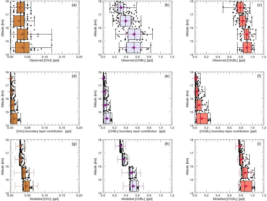
1166                     M. T. Filus et al.: Transport of short-lived halocarbons to the stratosphere over the Pacific Ocean

 iii. the initial concentration values for CH3 I, CHBr3 , and
      CH2 Br2 ;
                                                                                   X
                                                                    fractionBL =    (fractiont ),                               (4)
 iv. their atmospheric lifetimes (to account for the photo-         [X]BG_Contribution = (1 − fractionBL .) × [X]BG             (5)
     chemical removal along the trajectory).
More specifically, the boundary layer contribution to the TTL       Since each sample has 15 000 back-trajectories associated
for the VSL halocarbons is calculated using Eqs. (2) and (3):       with it, some of which came from below 1 km and some of
                                                                    which did not, a definition as to which air samples are con-
[X]BLContribution ,t = [X]BL × fractiont × exp(−t/τ ) ,      (2)    sidered a boundary layer and those that are considered back-
                                                                    ground is required. Two approaches are tested that use the
                        X
[X]BL_Contribution =       ([X]BLContribution ,t ).          (3)
                                                                    NAME calculations to identify AWAS samples in all flights
Equation (2) gives the boundary layer contribution to the           (2013 and 2014) with low convective influence by (i) fil-
TTL for a given tracer, X (where X could be CH3 I, CHBr3 ,          tering for air masses with boundary layer fraction values
CH2 Br2 ), at model output time step, t. The model output time      less than 1 %, 5 % or 10 % or by (ii) selecting the lowest
step used is 6 h, from t = 0 (particle release) to t = 48 (end of   10 % of boundary layer fractions. Following this, the CH3 I,
a 12 d run). [X]BL stands for the initial boundary layer con-       CHBr3 and CH2 Br2 AWAS observations, corresponding to
centration of a given tracer – assigned to each particle that       the boundary layer fraction values less than 1 %, 5 %, 10 %
crossed below 1 km (Table 1). Fractiont is a number of parti-       or the lowest 10 % of boundary layer fractions, are averaged
cles that first crossed 1 km in a model output time step, t, over   to provide CH3 I, CHBr3 and CH2 Br2 background mixing ra-
a total number of particles released, and exp(−t/τ ) is a term      tios. These two approaches are explored below (Sect. 3.1.2).
for the photochemical loss (where τ stands for atmospheric
lifetime of a respective VSL halocarbon). Equation (3) gives        2.3.3   The effect of assuming constant lifetimes
the boundary layer contribution that is the sum of boundary
layer contribution components in all model output time steps        The lifetimes of the halocarbons are not the same in the
(for t = 1 to 48).                                                  boundary layer and the TTL (Carpenter et al., 2014). The as-
    Equation (2) calculates the decay of each tracer after it       sumption of constant lifetime in a 12 d trajectory is evaluated
leaves the boundary layer (0–1 km), which is valid for a well-      by calculating the difference between idealized trajectories
mixed boundary layer. Since 15 000 particles are released for       that had 2, 4, 6, 8 and 10 d in the boundary layer and 10, 8, 6,
each AWAS sample, contributions from each particle from             4 and 2 d in the upper troposphere. Lifetimes for the bound-
below 1 km in the previous 12 d are summed. Decay times,            ary layer and for the upper troposphere for each gas were
τ , of 4, 15 and 94 d for CH3 I, CHBr3 and CH2 Br2 , respec-        taken from Carpenter et al. (2014). (Lifetimes for higher al-
tively, are used (i.e. constant chemical loss rate) (Carpenter      titudes are not available therein). The difference found be-
et al., 2014). Thus, a particle getting to the TTL in 1 d con-      tween the two extreme cases are 6 % (CHBr3 ), 3 % (CH2 Br2 )
tributes more of a given tracer to that air mass than a particle    and 25 % (CH3 I). The assumption is thus valid for the two
taking 10 d. Once this chemical loss term was taken into ac-        brominated species.
count, the NAME trajectories can be used to calculate the              This assumption is more robust than it might seem at first
contribution of convection of air masses from the boundary          glance. The boundary layer fraction is calculated using 12 d
layer within the preceding 12 d.                                    trajectories in which there is little loss of CH2 Br2 whether
    The initial boundary layer concentrations are derived from      a lifetime of 94 or 150 d is taken. The most important fac-
the CAST and CONTRAST WAS measurements taken in the                 tor in determining the amount lofted into the TTL is thus
western Pacific in the same period of January–March 2014 as         the original mixing ratio, which is only slightly modulated
for the ATTREX measurements in the TTL (Table 1). These             by the chemical loss in 12 d. The longer lifetime is absorbed
observed means are used in model calculations, and the simi-        implicitly and taken into account in the background contribu-
larity between them and literature values reported in Carpen-       tion. The same arguments apply for CHBr3 , though the effect
ter et al. (2014) is clear, with lower values for CHBr3 only.       is a bit larger. The largest difference is seen for CH3 I. How-
                                                                    ever, the difference matters much less for CH3 I because only
2.3.2   NAME-modelled background contribution                       4 %–5 % remains after the full 12 d, which is much smaller
                                                                    than the uncertainties in this analysis, so that much shorter
To compare our model results against the AWAS observa-              trajectories are used to validate the new convection scheme.
tions, the background contribution, [X]BG_Contribution (mean-
ing the contribution from the fraction of trajectories that do
not cross below 1 km within 12 d) needs to be accounted for.        3   Analysis of ATTREX 2014 research flight 02
This requires estimates for the fraction of trajectories from
the free troposphere, which is (1-fractionBL ), Eq. (4), and        We start by showing our results from a single ATTREX 2014
an estimate of the halocarbon mixing ratio in that fraction,        research flight, RF02, to illustrate the method. This is fol-
[X]BG , Eq. (5), i.e.                                               lowed by analysing all research flights together for ATTREX

Atmos. Chem. Phys., 20, 1163–1181, 2020                                               www.atmos-chem-phys.net/20/1163/2020/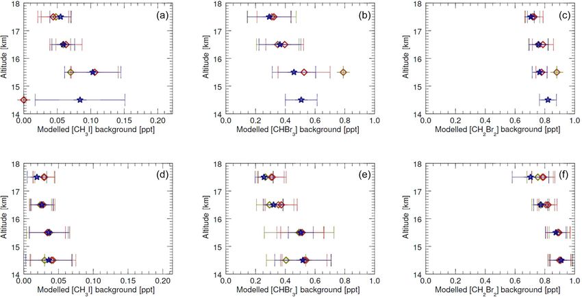
M. T. Filus et al.: Transport of short-lived halocarbons to the stratosphere over the Pacific Ocean 1167
Table 1. Boundary layer concentrations and atmospheric lifetimes for CH3 I, CHBr3 and CH2 Br2 (Carpenter et.al., 2014).
Tracer, Boundary layer concentration, Atmospheric life-
[X] [X]BL [ppt] time, τ [d]
CAST and CONTRAST Carpenter et al. (2014)
Mean (range) median Median (range)
CH3 I 0.70 (0.16–3.34) 0.65 0.8 (0.3–2.1) 4
CHBr3 0.83 (0.41–2.56) 0.73 1.6 (0.5–2.4) 15
CH2 Br2 0.90 (0.61-1.38) 0.86 1.1 (0.7-1.5) 94
2014 and 2013 in Sect. 4 and calculating the modelled con- tical uplift, while the second group has been in the upper
tribution of active bromine from CHBr3 and CH2 Br2 to the troposphere for longer than a couple of days (see Fig. 2c in
TTL (Sect. 5). Navarro et al., 2015, for a similar example). Above 16 km,
the overwhelming majority (> 90 %) of the released parti-
3.1 Individual ATTREX 2014 flight: research flight 02 cles are calculated to be in the TTL for the previous 12 d,
with negligible evidence for transport from the low tropo-
Figure 1 shows the vertical distribution of CH3 I, CHBr3 and sphere. This shows the dominance of the long-range, hor-
CH2 Br2 in the TTL observed during research flight, RF02, izontal transport for the 16–17 and 17–18 km NAME runs
during ATTREX 2014 (Table 4). Held on 16–17 Febru- (also shown in Navarro et al., 2015).
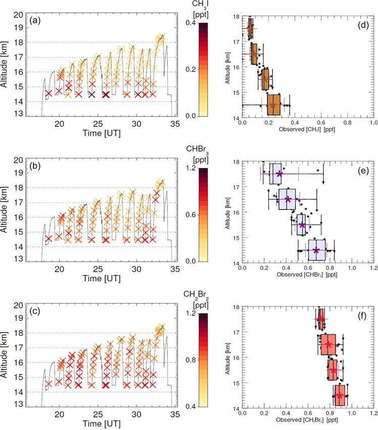
ary 2014, RF02 was conducted in a confined area east of Figure 3 shows the locations at which trajectories crossed
Guam (12–14◦ N, 145–147◦ E) due to a faulty primary satel- 1 km, thereby indicating boundary layer source regions for
lite communications system for Global Hawk command and the RF02 TTL air masses. Boundary layer sources in the
control (Jensen et al., 2017). A total of 26 vertical pro- western and central Pacific are the most important for the
files through TTL were made, with 86 AWAS measurements lowest TTL bin (14–15 km, Fig. 3a) in this flight. The Mar-
taken in total. A high degree of variability of CH3 I in the TTL itime Continent, the northern Australian coast, the Indian
was observed (from > 0.4 ppt at 14–15 km, to near-zero ppt Ocean and the equatorial band of the African continent in-
values at 17–18 km). Each profile, in general, showed a gra- crease in relative importance as altitude increases, though the
dation in CH3 I distribution in the TTL. Higher values were overall contribution of recent boundary layer air masses de-
measured in the lower TTL up to 16 km, with values decreas- creases with increasing altitude.
ing with altitude. The same pattern was observed for CHBr3 Figure 4 shows the NAME-modelled boundary layer con-
and CH2 Br2 , with the highest concentrations measured in the tribution to the TTL for CH3 I, CHBr3 and CH2 Br2 during
lower TTL (14–15 km) and the lowest at 17–18 km. RF02. It is important to note that this contribution corre-
sponds to uplift from below 1 km in the preceding 12 d, i.e.
3.1.1 NAME-modelled boundary layer contribution
the length of the trajectories. The calculated boundary layer
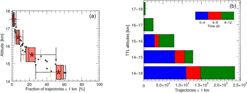
Figure 2a shows the vertical distribution of the boundary contributions for CH3 I, CHBr3 and CH2 Br2 from the 1 km
layer air contribution to the TTL (corresponding to the fractions are highest at 14–15 km, dropping off with alti-
AWAS measurement locations along the RF02 flight track). tude. Almost no boundary layer contribution is found for 17–
It reveals higher boundary layer air influence in the lower 18 km (with values close to 0 ppt).
TTL, decreasing with altitude (similar to the VSL halocar-
bon observations). Cumulatively, the highest fractions from 3.1.2 NAME-modelled background contribution
below 1 km are found for the lower TTL (14–15 km). A no-
ticeable decrease occurs between the lower and upper TTL Here we explore the two approaches summarized in
(15 to 17 km). From 16 km up, little influence (indicated by Sect. 2.3.2 for estimating the CHBr3 and CH2 Br2 back-
< 10 % and < 5 % 1 km fractions of trajectories below 1 km ground mixing ratios. Similar values are seen in ATTREX
for 16–17 and 17–18 km, respectively) of the low-level air 2013 and 2014. Less variation is observed for CH2 Br2 due to
masses is seen. its longer atmospheric lifetime.
Figure 2b shows all NAME runs for RF02 grouped into ATTREX 2013 and 2014 are treated separately in the anal-
four 1 km TTL bins: 14–15, 15–16, 16–17 and 17–18 km. In ysis presented below due to the difference in CH3 I back-
the 14–15 km bin, most particles from the low troposphere ground estimates. The approach using the lowest 10 % of the
arrived in the preceding 4 d with many in the preceding 2 d. boundary layer fractions is used to estimate the background
This represents the fast vertical uplift of the low tropospheric contribution for the 2014 flights as not enough data meet the
air masses to the lower TTL. At 15–16 km, two particle pop- former condition due to the proximity of the flights to strong
ulations are observed: the first group results from recent ver- convection. The background values, inferred from all the AT-
www.atmos-chem-phys.net/20/1163/2020/ Atmos. Chem. Phys., 20, 1163–1181, 2020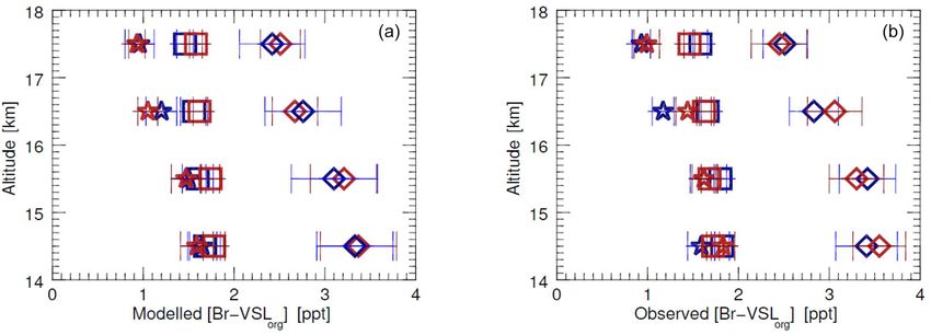
1168                      M. T. Filus et al.: Transport of short-lived halocarbons to the stratosphere over the Pacific Ocean

Figure 1. Vertical distribution of CH3 I, CHBr3 and CH2 Br2 in the TTL, as measured during research flight 02, ATTREX 2014. AWAS
measurements along the flight track (a–b) and observations grouped into 1 km TTL segments (d–f): mean (star symbols), standard deviation
(coloured whiskers), minimum, lower and upper quartiles, median, and maximum (black box and whiskers).

Figure 2. Vertical distribution of NAME 1 km fractions (the fractions that reach the boundary layer within 12 d – indicative of boundary layer
air influence) in the TTL (a). Distribution of transport times taken for the trajectories to first cross below 1 km (reach the boundary layer) for
all the NAME runs and the NAME runs grouped into 1 km TTL segments, research flight 02, ATTREX 2014 (b).

Atmos. Chem. Phys., 20, 1163–1181, 2020                                                        www.atmos-chem-phys.net/20/1163/2020/
M. T. Filus et al.: Transport of short-lived halocarbons to the stratosphere over the Pacific Ocean                                1169

Figure 3. Crossing location distribution maps for all the NAME runs released from four 1 km TTL altitudes between 14 and 18 km. Strong
influence of local boundary air is noted for a 14–15 km segment (lower TTL), whereas the boundary air from remote locations dominates for
a 17–18 km segment (upper TTL), research flight 02, ATTREX 2014.

Figure 4. NAME-modelled CH3 I, CHBr3 and CH2 Br2 boundary layer contribution to the TTL, research flight 02, ATTREX 2014.

TREX 2014 flights, are used in the individual flight calcula-          TREX 2013, low CH3 I background mixing ratios are found.
tions as again there are not enough data from an individual            All approaches show similar background mixing ratios. In
flight to make background calculations for that flight. In AT-         2014, higher CH3 I background mixing ratios are calculated
TREX 2013 we use the boundary layer fractions less than                due to ubiquity of air from recent, vertical uplift. No bound-
5 % approach for the CH3 I background estimation. The AT-              ary layer fractions less than 1 % are found for the 14–17 km
TREX 2014 background estimates should be taken as upper                bins and none less than 5 % are found for the 14–15 km bins.
limits as it is hard to identify samples with no convective in-
fluence in 2014. This is especially true for the lower TTL             3.1.3   NAME-modelled total concentrations
since the ATTREX 2014 flights were close to the region of
strong convection.                                                     The NAME boundary layer and background contribution es-
   Figure 5 shows the VSL background mixing ratios calcu-              timates are added to give an estimate for total halocarbon
lated for the ATTREX campaigns in 2013 and 2014. In AT-                mixing ratio, [X]NAME_TTL , (Eq. 1), for comparison with the
                                                                       AWAS observations.

www.atmos-chem-phys.net/20/1163/2020/                                                    Atmos. Chem. Phys., 20, 1163–1181, 2020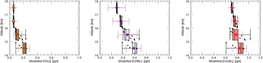
1170                    M. T. Filus et al.: Transport of short-lived halocarbons to the stratosphere over the Pacific Ocean

Figure 5. Background mixing ratios for CH3 I, CHBr3 and CH2 Br2 for all NAME runs for all flights in ATTREX 2014 (a–c) and ATTREX
2013 (a–f). Little convective influence is indicated by selecting means from NAME 1 km fractions of < 1 (blue star), 5 (red diamond) and
10 % (green diamond).

   Figure 6 and Table 2 show the vertical distribution of             4   The role of transport in the VSL halocarbon
NAME-based estimates for CH3 I, CHBr3 and CH2 Br2 in the                  distribution in the TTL
TTL for RF02. The sums of the NAME CH3 I, CHBr3 and
CH2 Br2 boundary layer and background contribution esti-              The role of transport in the CH3 I, CHBr3 and CH2 Br2 dis-
mates agree well with the AWAS observations for all the               tribution in the TTL is examined in this section by apply-
1 km TTL bins (compared with Fig. 1).                                 ing the NAME-based analysis introduced in Sect. 3 to all
   At 14–15 km, the modelled boundary layer contribution of           CH3 I, CHBr3 and CH2 Br2 AWAS observations in the AT-
CH3 I is similar to the observations, indicating recent, rapid        TREX 2013 and 2014 campaigns.
convective uplift. This provides evidence that the improved              In ATTREX 2013, six flights surveyed the eastern Pacific
convection scheme provides a realistic representation of par-         TTL in February–March 2013. Four flights went west from
ticle displacement via deep convection. At higher altitudes,          Dryden Flight Research Centre to the area south of Hawaii,
the background contribution is more important and, indeed,            reaching 180◦ longitude. Little influence of convective activ-
the modelled total CH3 I values are greater than the observa-         ity was observed. Most samples with strong boundary layer
tions. This overestimate of the background contribution re-           influence were observed in air masses that had originated
sults from the difficulty of identifying samples with no con-         over the western Pacific and the Maritime Continent, where it
vective influence in ATTREX 2014. This problem is most                was uplifted to the TTL and transported horizontally within
important for CH3 I with its very short lifetime.                     the TTL (Navarro et al., 2015). Two flights sampled the TTL
   CHBr3 drops off slower with altitude than CH3 I and                near the Central American and South American coasts. Few
quicker than CH2 Br2 . At 14–15 km, the boundary layer                convective episodes were observed. The sampled air predom-
contribution accounts for ∼ 50 % of the modelled sums of              inantly had a small boundary layer air signature from the
CHBr3 and CH2 Br2 but less than 5 % for CHBr3 and CH2 Br2             western Pacific and the Maritime Continent.
at 17–18 km. For the upper TTL, the background contribu-                 In ATTREX 2014, two transit flights and six research
tion estimates constitute over 85 % of the modelled sums,             flights were made in the western Pacific in January–
thus taking on more importance.                                       February 2014. This period coincided with the active phase
                                                                      of the Madden–Julian Oscillation (MJO) and increased activ-
                                                                      ity of tropical cyclones. A large influence of recent convec-
                                                                      tive events is observed (Navarro et al., 2015), reflected in the
                                                                      elevated CH3 I and CHBr3 mixing ratios and the high values

Atmos. Chem. Phys., 20, 1163–1181, 2020                                                 www.atmos-chem-phys.net/20/1163/2020/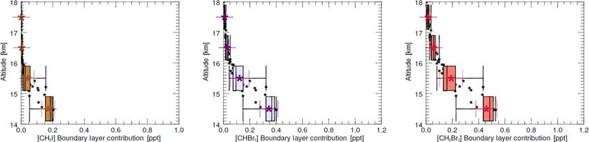
M. T. Filus et al.: Transport of short-lived halocarbons to the stratosphere over the Pacific Ocean 1171
Figure 6. Vertical distribution of NAME-modelled CH3 I, CHBr3 and CH2 Br2 (sums of boundary layer and background contribution) in the
TTL for research flight 02, ATTREX 2014.
of NAME fractions of trajectories below 1 km. All three air-
craft flew together in 2014, thus there is a more complete set
of measurements from the ground up. Accordingly, this year
is discussed first.
Table 2. ATTREX 2014 research flight 02. AWAS observations;
modelled boundary layer contribution; and the modelled total mix- 4.1 VSL halocarbon distribution in the TTL: ATTREX
ing ratios for CH3 I, CHBr3 , and CH2 Br2 . The boundary layer and 2014
background fraction means and standard deviations (in brackets) are
given based on the measurements and modelled values for the sam- Figure 7 shows the vertical distribution of the observations
ples collected during the flight. and of the modelled boundary layer contribution and total
mixing ratios for CH3 I, CHBr3 and CH2 Br2 for all the AT-
Altitude AWAS Modelled boundary Modelled total TREX 2014 flights (using only the AWAS measurements
[km] [ppt] layer contribution mixing ratio
made from 20◦ N southward). As in RF02, CH3 I is highest
[ppt] [ppt]
in the lower TTL, dropping off with altitude. Large flight-
CH3 I to-flight variability in CH3 I measurements is seen. The frac-
17–18 0.06 (0.02) 0.00 (0.00) 0.06 (0.02) tion of NAME particles that travel below 1 km in the previ-
16–17 0.09 (0.03) 0.00 (0.00) 0.06 (0.02) ous 12 d (Table 3) are highest at 14–15 km (mean of 57 %)
15–16 0.17 (0.03) 0.04 (0.04) 0.12 (0.06) and decrease with altitude in a similar fashion. The CH3 I
14–15 0.23 (0.09) 0.17 (0.04) 0.21 (0.08)
boundary layer contribution explains most of the observa-
CHBr3 tions for the 14–15 and 15–16 km layers. Disparities in ob-
17–18 0.34 (0.17) 0.01 (0.00) 0.29 (0.15) served and modelled CH3 I arise from 16 km upwards. Esti-
16–17 0.42 (0.11) 0.03 (0.01) 0.36 (0.14) mated background values are very low, oscillating between
15–16 0.55 (0.06) 0.12 (0.07) 0.48 (0.17) 0 and the limit of detection of the AWAS instrument for the
14–15 0.67 (0.10) 0.35 (0.07) 0.58 (0.13) iodinated short-lived organic substances, 0.01 ppt. The sums
CH2 Br2 of the CH3 I boundary layer and background contribution es-
17–18 0.72 (0.02) 0.02 (0.01) 0.71 (0.03)
timates show good agreement with AWAS observations for
16–17 0.79 (0.07) 0.06 (0.02) 0.76 (0.06) all the TTL 1 km segments (Table 3).
15–16 0.83 (0.05) 0.19 (0.09) 0.78 (0.10) The good agreement for the 14–15 and 15–16 km layers
14–15 0.89 (0.05) 0.46 (0.08) 0.84 (0.12) can be attributed to the improved representation of deep con-
Boundary layer Background vection in NAME, provided by the new convection scheme
fraction [%] fraction [%] (Meneguz et al., 2019). However, there is an underestimation
17–18 2.1 (1.1) 97.9
of the boundary layer contribution to the upper TTL levels
16–17 7.2 (2.7) 92.8 (16–17 and 17–18 km), which we attribute to the new con-
15–16 22.9 (10.0) 77.1 vection scheme not working as well at these altitudes. This
14–15 53.3 (9.0) 46.7 is consistent with a known tendency of the unified model to
underestimate the depth of deepest convection in the tropics
(Walters et al., 2019). Both the CH3 I AWAS observations and
the modelled sums are higher than reported previously in the
literature (Carpenter et al., 2014) for all the TTL segments.
This may be explained by sampling the TTL in a region of
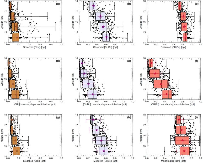
www.atmos-chem-phys.net/20/1163/2020/ Atmos. Chem. Phys., 20, 1163–1181, 20201172 M. T. Filus et al.: Transport of short-lived halocarbons to the stratosphere over the Pacific Ocean Figure 7. CH3 I, CHBr3 and CH2 Br2 vertical distribution in the TTL for ATTREX 2014 flights.: AWAS observations (a–c), NAME-modelled boundary layer contribution (d–f), and NAME-modelled sums of boundary layer and background contributions (g–i). high convective activity. This result gives confidence in the 4.2 VSL halocarbon distribution in the TTL: ATTREX quality of the new convection scheme and hence in simi- 2013 lar calculations of convective influence on the longer-lived CHBr3 and CH2 Br2 . The highest CHBr3 and CH2 Br2 concentrations were ob- Figure 8 shows the vertical distribution for CH3 I, CHBr3 and served in the lower TTL (14–15 km), dropping off more CH2 Br2 in the TTL observed and modelled from the AT- slowly with altitude than CH3 I. The weight of the modelled TREX 2013 flights. Only AWAS measurements taken south boundary layer contribution estimates to the modelled to- of 20◦ N are used. Much lower CH3 I values are found in tal amounts varies from approximately 50 % at 14–15 km 2013 than in 2014 (Fig. 7). The NAME 1 km fractions are (unlike for CH3 I where over 85 % of the modelled sum is considerably lower (∼ 4-fold), and the corresponding CH3 I attributed to the boundary layer contribution at 14–15 km) boundary layer contribution shows values close to the limit to < 20 % at 17–18 km. The sums of the modelled bound- of detection of the AWAS instrument for CH3 I. The back- ary layer and background contributions are in good agree- ground contribution comprises over 85 %–90 % of the sums ment with the CHBr3 and CH2 Br2 AWAS observations. The of the modelled CH3 I estimate in the TTL. Good agreement ATTREX observations and the NAME-modelled sums are is found between the AWAS observations and the sum of within the range of values reported in the literature (Carpen- the modelled boundary layer and background contributions. ter et al., 2014). Both the observed and modelled values are in the low end of Atmos. Chem. Phys., 20, 1163–1181, 2020 www.atmos-chem-phys.net/20/1163/2020/
M. T. Filus et al.: Transport of short-lived halocarbons to the stratosphere over the Pacific Ocean                               1173

Table 3. ATTREX 2014 all flights. AWAS observations; modelled           ATTREX 2013 was in the eastern Pacific away from the main
boundary layer contribution; and the modelled total mixing ratios       region of strong convection. Longer transport timescales re-
for CH3 I, CHBr3 , and CH2 Br2 . The boundary layer and back-           sult from horizontal transport and were more important in
ground fractions are also given. Means and standard deviations are      ATTREX 2013, with much less recent convective influence
given in brackets.                                                      than in ATTREX 2014. More chemical removal of CH3 I and
                                                                        CHBr3 thus took place, leading to lower concentrations in
  Altitude       AWAS        Modelled boundary         Modelled total
                                                                        the eastern Pacific TTL.
  [km]            [ppt]       layer contribution        mixing ratio
                                           [ppt]               [ppt]
                                                                           The trajectories are analysed to investigate the timescales
                                                                        for vertical transport by calculating how long it took parti-
  CH3 I                                                                 cles to go from below 1 km to the TTL. In 2013, almost no
  17–18      0.04 (0.03)                 0.02 (0.03)      0.07 (0.04)   episodes of recent rapid vertical uplift are found, with most
  16–17      0.11 (0.10)                 0.04 (0.04)      0.09 (0.05)   particles taking 8 d and more to cross the 1 km. This is indica-
  15–16      0.16 (0.14)                 0.09 (0.07)      0.15 (0.08)   tive of the dominant role of long-range horizontal transport.
  14–15      0.17 (0.14)                 0.15 (0.08)      0.19 (0.11)   In 2014, by way of contrast, a considerable number of tra-
  CHBr3                                                                 jectories (tenths of a percent) come from below 1 km in less
                                                                        than 4 d, representing the “young” air masses being brought
  17–18      0.33 (0.14)                 0.06 (0.06)      0.32 (0.16)
                                                                        from the low troposphere via recent and rapid vertical uplift.
  16–17      0.48 (0.13)                 0.12 (0.09)      0.40 (0.17)
  15–16      0.54 (0.13)                 0.21 (0.12)      0.50 (0.19)
                                                                           The spatial variability in the boundary layer mixing ra-
  14–15      0.61 (0.13)                 0.31 (0.12)      0.55 (0.16)   tios corresponding to different source strengths coupled with
                                                                        the variation in atmospheric transport pathways and trans-
  CH2 Br2                                                               port timescales can explain the differences in the distribution
  17–18      0.73 (0.06)                 0.11 (0.09)      0.73 (0.09)   of the NAME 1 km fractions in the TTL. In 2014 (2013),
  16–17      0.82 (0.08)                 0.19 (0.14)      0.78 (0.15)   higher (lower) boundary layer fractions corresponded well
  15–16      0.84 (0.09)                 0.32 (0.16)      0.80 (0.17)   with higher (lower) CH3 I and CHBr3 values in the TTL, es-
  14–15      0.86 (0.07)                 0.44 (0.15)      0.84 (0.17)   pecially with the highest concentrations occurring for the
                      Boundary layer                     Background     flights with the most convective influence and the highest
                       fraction [%]                      fraction [%]   fractions of particles arriving within the 4 d.
  17–18                    12.7 (10.9)                          87.3       In 2014, the western and central Pacific is the dominant
  16–17                    22.3 (16.0)                          77.7    source origin of boundary layer air to the TTL (Navarro et
  15–16                    37.8 (18.8)                          62.2    al., 2015). Increased tropical cyclone activity in this area
  14–15                    51.7 (16.1)                          48.3    (particularly Faxai, 28 February–6 March 2014, and Lusi,
                                                                        7–17 March 2014) and the strong signal from convection
                                                                        related to the Madden Julian Oscillation (MJO – an in-
the CH3 I concentrations reported by the WMO 2014 Ozone                 traseasonal phenomenon characterized by an eastward spread
Assessment (Carpenter et al., 2014).                                    of large regions of enhanced and suppressed tropical rain-
   The ATTREX 2013 mixing ratios are lower for CHBr3 and                fall, mainly observed over the Indian and Pacific Ocean)
higher CH2 Br2 than shown in Fig. 7 for 2014. The NAME-                 contributed to the more frequent episodes of strong and
calculated CHBr3 and CH2 Br2 boundary layer contributions               rapid vertical uplifts of the low-level air to the TTL. A sig-
are small, constituting approximately 10 % of the NAME-                 nificant contribution is also seen from the central Indian
modelled sums for 14–15 km and less for the upper TTL                   Ocean, marking the activity of Tropical Cyclone Fobane
segments. The background contribution estimates comprise                (6–14 February 2014). Minimal contribution from the other
over 85 % of the modelled sums. Good agreement is found                 remote sources (Indian Ocean, African continental tropical
between the sums of the modelled boundary layer and back-               band) is found (Anderson et al., 2016; Jensen et al., 2017;
ground contributions and the CHBr3 and CH2 Br2 AWAS ob-                 Newton et al., 2018).
servations.

4.3   ATTREX 2013 and 2014: inter-campaign                              5   How much do VSL bromocarbons contribute to the
      comparison                                                            bromine budget in the TTL?

Clear differences in the vertical distributions of CH3 I in the         The NAME-modelled CHBr3 and CH2 Br2 estimates in the
TTL are found in ATTREX 2013 and 2014. CH3 I estimates,                 TTL are used to calculate how much bromine from the VSL
corresponding to high values in the NAME-modelled 1 km                  bromocarbons, Br-VSLorg , is found in the lower stratosphere,
fractions, are high in 2014, whereas in 2013 almost no CH3 I            based on how much enters the TTL in the form of bromo-
is estimated to be in the TTL. This is due to the minimal con-          carbons (Navarro et al., 2015). CHBr3 and CH2 Br2 are the
tribution of the boundary layer air within the previous 12 d:           dominant short-lived organic bromocarbons, and the minor

www.atmos-chem-phys.net/20/1163/2020/                                                    Atmos. Chem. Phys., 20, 1163–1181, 2020
1174 M. T. Filus et al.: Transport of short-lived halocarbons to the stratosphere over the Pacific Ocean Figure 8. CH3 I, CHBr3 and CH2 Br2 vertical distribution in the TTL for ATTREX 2013 flights: AWAS observations (a–c), NAME-modelled boundary layer contribution (d–f), and NAME-modelled sums of boundary layer and background contributions (g–i). bromocarbons, CH2 BrCl, CHBr2 Cl and CHBrCl2 , are ex- Good agreement is found between the bromine loading cluded here (their combined contribution is less than 1 ppt to from the VSL bromocarbons, inferred from the NAME- Br-VSLorg at 14–18 km, Navarro et al., 2015). The NAME- modelled estimates initialized with BAe-146 and GV mea- modelled CHBr3 and CH2 Br2 estimates are multiplied by surements, and the Global Hawk AWAS observations. the number of bromine atoms (bromine atomicity) and then Higher organic bromine loading is seen around the cold point summed to yield the total of Br-VSLorg . tropopause (16–17 km) in ATTREX 2014. Figure 9 shows the contribution of CHBr3 and CH2 Br2 , Using the upper troposphere measurements taken during the two major VSL bromocarbons contributing to the the SHIVA campaign in the western Pacific in November– bromine budget in the TTL. For ATTREX 2013 and 2014, December 2011, Sala et al. (2014) calculated an estimate similar contributions of CHBr3 and CH2 Br2 to Br-VSLorg for VSL (CHBr3 , CH2 Br2 , CHBrCl2 , CH2 BrCl, CHBr2 Cl) are found in the lower TTL. In 2014, CHBr3 in the lower contributions to the organic bromine at the level of zero TTL was abundant enough to contribute as much Br-VSLorg radiative heating (15.0–15.6 km). Air masses reaching this as CH2 Br2 . A combination of larger boundary layer air in- level are expected to reach the stratosphere. This VSL fluence in the TTL and shorter mean transport times to reach mean mixing ratio estimate of 2.88 (±0.29) ppt (2.35 ppt the TTL result in the observed higher CHBr3 contribution to for CHBr3 and CH2 Br2 , excluding minor short-lived bromo- the Br-VSLorg in the lower TTL in 2014, than in 2013. The carbons) is lower due to a lower contribution from CHBr3 CH2 Br2 contribution dominates in the upper TTL due to its estimate (0.22 ppt compared to the CHBr3 estimate for longer atmospheric lifetime. NAME/ATTREX in Table 5). Our estimates of the contri- Atmos. Chem. Phys., 20, 1163–1181, 2020 www.atmos-chem-phys.net/20/1163/2020/
M. T. Filus et al.: Transport of short-lived halocarbons to the stratosphere over the Pacific Ocean                                   1175

Figure 9. Contribution of CHBr3 (star symbol) and CH2 Br2 (square symbol) to the bromine budget in the TTL, inferred from the NAME-
modelled estimates (a) and AWAS observations (b); ATTREX 2014 (red) and 2013 (blue) are shown separately. Stars and square symbols
represent the bromine atomicity products from CHBr3 and CH2 Br2 , respectively. Diamonds show the bromine contribution from the VSL
bromocarbons in the TTL (as a sum of the CHBr3 and CH2 Br2 bromine atomicity products).

bution of CHBr3 and CH2 Br2 to the organic bromine at the
Level of Zero Radiative Heating (LZRH) are largely slightly
higher than those in Sala et al. (2014) due to a higher estimate
for a shorter-lived CHBr3 .                                         Table 4. ATTREX 2013 all flights. AWAS observations; modelled
   Several papers use the same measurements from the com-           boundary layer contribution; and the modelled total mixing ratios
bined ATTREX/CAST/CONTRAST campaign in 2014 and                     for CH3 I, CHBr3 , and CH2 Br2 . The boundary layer and back-
from the other ATTREX phases. Navarro et al. (2015) re-             ground fractions are also given. Means and standard deviations are
port slightly higher bromine loading from the Br-VSLorg             given in brackets.
at the tropopause level (17 km) in the western Pacific in
2014 than in the eastern Pacific in 2013 (the Br-VSLorg val-          Altitude       AWAS        Modelled boundary         Modelled total
ues from the AWAS observations were of 3.27 ppt, ±0.47,               [km]            [ppt]       layer contribution        mixing ratio
and 2.96 ppt, ±0.42, respectively). The minor short-lived or-                                                  [ppt]               [ppt]
ganic bromine substances were included in the analysis of             CH3 I
Navarro et al. (2015), accounting for the higher Br-VSLorg .
                                                                      17–18      0.03 (0.02)                 0.00 (0.00)      0.03 (0.01)
Butler et al. (2018), report a mean mole fraction and range           16–17      0.03 (0.02)                 0.00 (0.00)      0.03 (0.02)
of 0.46 (0.13–0.72) ppt and 0.88 (0.71–1.01) ppt of CHBr3             15–16      0.04 (0.02)                 0.01 (0.01)      0.03 (0.03)
and CH2 Br2 , respectively, being transported to the TTL dur-         14–15      0.04 (0.03)                 0.01 (0.01)      0.05 (0.03)
ing January and February 2014. This is consistent with a
                                                                      CHBr3
contribution of 3.14 (1.81–4.18) ppt of organic bromine to
the TTL over the region of the campaign. The analysis of              17–18      0.31 (0.10)                 0.01 (0.01)      0.31 (0.09)
the injection of brominated VSLs into the TTL by Wales et             16–17      0.39 (0.12)                 0.02 (0.02)      0.35 (0.11)
al. (2018) using the CAM-chem-SD model combined with a                15–16      0.54 (0.15)                 0.04 (0.04)      0.49 (0.16)
                                                                      14–15      0.53 (0.15)                 0.07 (0.05)      0.53 (0.18)
steady-state photochemical box model and CONTRAST and
ATTREX data found that 2.9 ± 0.6 ppt of bromine enters the            CH2 Br2
stratosphere via organic source gas injection of VSLs. The            17–18      0.79 (0.08)                 0.02 (0.04)      0.78 (0.07)
NAME-modelled results presented here (Fig. 9, Table 5) are            16–17      0.83 (0.07)                 0.04 (0.04)      0.81 (0.07)
thus in good agreement with the values reported by Navarro            15–16      0.90 (0.07)                 0.07 (0.06)      0.87 (0.10)
et al. (2015), Butler et al. (2018) and Wales et al. (2018).          14–15      0.91 (0.08)                 0.12 (0.09)      0.89 (0.12)
                                                                                          Boundary layer                     Background
                                                                                           fraction [%]                      fraction [%]
6   Summary and discussion
                                                                      17–18                     1.9 (2.3)                           98.1
                                                                      16–17                     4.7 (4.9)                           95.3
We have used the NAME trajectory model in backward mode               15–16                     9.8 (7.9)                           90.2
to assess the contribution of recent convection to the mix-           14–15                    14.7 (11.1)                          85.3
ing ratios of three short-lived halocarbons, CH3 I, CHBr3 and
CH2 Br2 . The 15 000 back-trajectories are computed for each
measurement made with the whole air samples on the NASA
Global Hawk in ATTREX 2013 and 2014, and the fraction

www.atmos-chem-phys.net/20/1163/2020/                                                Atmos. Chem. Phys., 20, 1163–1181, 2020
1176 M. T. Filus et al.: Transport of short-lived halocarbons to the stratosphere over the Pacific Ocean
Table 5. Contribution from the very short-lived bromocarbons: CHBr3 and CH2 Br2 to the bromine in the TTL, as given by modelled
estimates and AWAS observations for ATTREX 2014 and 2013. [CHBr3 ] and [CH2 Br2 ] means are shown.
Altitude [km] [CHBr3 ] [CH2 Br2 ] Br from CHBr3 Br from CH2 Br2 Br-VSLorg
[ppt] [ppt] [ppt] [ppt] [ppt]
ATTREX 2014
NAME
17–18 0.32 0.73 0.96 1.46 2.42
16–17 0.40 0.78 1.20 1.56 2.76
15–16 0.50 0.80 1.50 1.60 3.10
14–15 0.55 0.84 1.65 1.68 3.33
AWAS
17–18 0.33 0.73 0.99 1.46 2.45
16–17 0.48 0.82 1.44 1.64 3.08
15–16 0.54 0.84 1.62 1.68 3.30
14–15 0.61 0.86 1.83 1.72 3.55
ATTREX 2013
NAME
17–18 0.31 0.78 0.93 1.56 2.49
16–17 0.35 0.81 1.05 1.62 2.67
15–16 0.49 0.87 1.47 1.74 3.21
14–15 0.53 0.89 1.59 1.78 3.37
AWAS
17–18 0.31 0.79 0.93 1.58 2.51
16–17 0.39 0.83 1.17 1.66 2.83
15–16 0.54 0.90 1.62 1.80 3.42
14–15 0.53 0.91 1.59 1.82 3.41
that originated below 1 km is calculated for each sample. A very few NAME trajectories passed below 1 km. This is pos-
steep drop-off in this fraction is observed between 14–15 and sible in 2013 when the ATTREX flights were away from the
17–18 km. Low-level measurements of CH3 I, CHBr3 and region of strong convection but much harder in 2014 when
CH2 Br2 from the FAAM BAe-146 and the NCAR GV are (as planned!) the flights were heavily influenced by convec-
used in conjunction with these trajectories and an assumed tion. By summing the boundary layer and background con-
photochemical decay time to provide estimates of the amount tributions, an estimate of the total bromocarbon mixing ratio
of each gas reaching the TTL from below 1 km. Compari- is obtained.
son of these modelled estimates with the CH3 I measurements The resulting modelled estimates are found to be in gen-
shows good agreement with the observations at the lower al- erally good agreement with the ATTREX measurements. In
titudes in the TTL values, with less good agreement at al- other words, a high degree of consistency is found between
titudes > 16 km, though it should be noted that the amounts the low-altitude halocarbon measurements made on the BAe-
are very small here. The lifetime of CH3 I is 3–5 d and thus 146 and GV and the high-altitude measurements made on
there is a > 90 % decay in the 12 d trajectories. The compari- the Global Hawk when they are connected using trajectories
son between the modelled and measured CH3 I thus indicates calculated by the NAME dispersion model with its updated
that the NAME convection scheme is realistic up to the lower convection scheme and driven by meteorological analyses
TTL but less good at reproducing the small number of ex- with 25 km horizontal resolution. There are some indications
treme convective events that penetrate to the upper TTL. of the modelled convection not always reaching quite high
In order to perform similar calculations for the longer- enough, but this is consistent with a known tendency of the
lived bromocarbons, an estimate of the background free- Unified Model to underestimate the depth of the deepest con-
tropospheric concentration is required. This is found by con- vection in the tropics.
sidering bromocarbon values in samples where there was The resolved winds are likely to be well represented, at
only a small influence from the boundary layer, i.e. where least partly because the wind data are analyses rather than
Atmos. Chem. Phys., 20, 1163–1181, 2020 www.atmos-chem-phys.net/20/1163/2020/M. T. Filus et al.: Transport of short-lived halocarbons to the stratosphere over the Pacific Ocean 1177
forecast data. Hence, we expect the main errors in the mod- Data availability. The CH3 I, CHBr3 and CH2 Br2 AWAS data
elling to arise from the representation of convection. Individ- from the NASA ATTREX measurements are available on-
ual convective events are hard to model and can have signifi- line in the NASA ATTREX database (https://espoarchive.
cant errors. However, because the upper troposphere concen- nasa.gov/archive/browse/attrex/id4, last access: 22 April 2017).
trations depend on a number of convective events and we are The CAST measurements are stored on the British Atmo-
spheric Data Centre, which is part of the Centre for En-
considering a range of flights and measurement locations, our
vironmental Data archive at http://catalogue.ceda.ac.uk/uuid/
conclusions on general behaviour should be robust. The con- 565b6bb5a0535b438ad2fae4c852e1b3 (Natural Environment Re-
sistency between the aircraft measurements and the NAME search Council et al., 2014). The CONTRAST AWAS data are
simulations supports this. available through https://data.eol.ucar.edu/master_lists/generated/
In the above, the boundary layer contribution arises from contrast/ (last access: 30 January 2020). The NAME data are avail-
trajectories that visit the boundary layer within 12 d while able from the corresponding author upon request. Please note that
the background contribution involves air that has been trans- the full paper is accessible upon request, contact David Thomson
ported into the TTL from outside the boundary layer on from the UK Met Office, Atmospheric Dispersion and Air Quality
timescales up to 12 d. Sensitivity tests were performed in Unit.
which the trajectories were followed for longer than 12 d:
the effect was to re-allocate some of the air from the back-
ground category into the boundary layer contribution with no Author contributions. The main part of the analysis was conducted
net change in the total. by MTF. ELA and MAN provided CH3 I, CHBr3 and CH2 Br2
AWAS measurements from the ATTREX and CONTRAST research
The approach using NAME trajectories and boundary
flights. SJA and LJC provided CH3 I, CHBr3 and CH2 Br2 mea-
layer measurements produces Br-VSLorg estimates of 3.5 ±
surements from the CAST campaign. MJA designed initial scripts
0.4 (3.3 ± 0.4) ppt in the lower eastern (western) Pacific TTL for NAME runs and products. EM and DT developed the model
(14–15 km) and 2.5 ± 0.2 (2.4 ± 0.4) ppt in the upper eastern code for improved convection scheme. MTF and NRPH prepared
(western) Pacific TTL (17–18 km). These lie within the range the manuscript with contributions from all co-authors, NRPH also
of the recent literature findings (Tegtmeier et al., 2012; Car- supervised this PhD work.
penter et al., 2014; Liang et al., 2014; Navarro et al., 2015;
Butler et al., 2018; Wales et al. 2018). The validation with
the ATTREX measurements provides confidence that a simi- Competing interests. The authors declare that they have no conflict
lar approach could be used for years when high-altitude mea- of interest.
surements are not available, assuming that realistic estimates
of the background tropospheric contributions can be obtained
from either models or measurements. Acknowledgements. The authors would like to thank our
Our study of boundary layer contribution of bromoform NASA ATTREX, NCAR CONTRAST and NERC CAST project
and dibromomethane into the TTL in the western Pacific, us- partners and their technical teams. Michal T. Filus would like to
thank Michelle Cain, Alex Archibald, Sarah Connors, Maria Russo
ing a combined approach of NAME Lagrangian dispersion
and Paul Griffiths for their input on the NAME applications for
modelling and CAST, CONTRAST and ATTREX 2014 mea- flight planning and post-flight modelling. We acknowledge use of
surements, has successfully validated an updated convection the NAME atmospheric dispersion model and associated NWP
scheme for use with the NAME trajectory model. The pre- meteorological datasets made available to us by the UK Met Office.
vious parameterization scheme was reasonable for convec-
tion at mid-latitudes but was far too weak to represent the
stronger tropical convection. Comparison with the extensive Financial support. The research was funded through the UK
CH3 I measurements made in this campaign provides good Natural Environment Research Council CAST project (grant
support for its use in modelling transport in tropical convec- nos. NE/J006246/1 and NE/J00619X/1), and Michal T. Filus was
tive systems (Meneguz et al., 2019). supported by a NERC PhD studentship. Elliot L. Atlas received sup-
This represents a considerable improvement on the ear- port from NASA (grant nos. NNX17AE43G, NNX13AH20G, and
lier study by Ashfold et al. (2012), which used the old con- NNX10AOB3A).
vection scheme and found reasonable agreement up to and
including the level of maximum convective outflow but not
above, when compared to measurements in the eastern Pa- Review statement. This paper was edited by Rolf Müller and re-
viewed by two anonymous referees.
cific from the NASA Costa Rica-Aura Validation Experiment
(CR-AVE, 2006) and NASA Tropical Composition, Cloud
and Climate Coupling (TC4, 2007) campaigns. The approach
used by Ashfold et al. (2012) has been further extended so
that VSL mixing ratios can be assigned to contributions from
the boundary layer and from the “background” TTL.
www.atmos-chem-phys.net/20/1163/2020/ Atmos. Chem. Phys., 20, 1163–1181, 2020You can also read